software implementation running on a general purpose mi- croprocessor. ... by means of feedback. Initially, a math- emat
An FPGA Implementation of a Sparse Quadratic Programming Solver for Constrained Predictive Control Juan L. Jerez Department of Electrical and Electronic Engineering Imperial College London SW7 2AZ, United Kingdom
[email protected]
George A. Constantinides Department of Electrical and Electronic Engineering Imperial College London SW7 2AZ, United Kingdom
Eric C. Kerrigan Department of Electrical and Electronic Engineering Department of Aeronautics Imperial College London SW7 2AZ, United Kingdom
[email protected]
[email protected]
ABSTRACT
1.
Model predictive control (MPC) is an advanced industrial control technique that relies on the solution of a quadratic programming (QP) problem at every sampling instant to determine the input action required to control the current and future behaviour of a physical system. Its ability in handling large multiple input multiple output (MIMO) systems with physical constraints has led to very successful applications in slow processes, where there is sufficient time for solving the optimization problem between sampling instants. The application of MPC to faster systems, which adds the requirement of greater sampling frequencies, relies on new ways of finding faster solutions to QP problems. Field-programmable gate arrays (FPGAs) are specially well suited for this application due to the large amount of computation for a small amount of I/O. In addition, unlike a software implementation, an FPGA can provide the precise timing guarantees required for interfacing the controller to the physical system. We present a high-throughput floating-point FPGA implementation that exploits the parallelism inherent in interior-point optimization methods. It is shown that by considering that the QPs come from a control formulation, it is possible to make heavy use of the sparsity in the problem to save computations and reduce memory requirements by 75%. The implementation yields a 6.5x improvement in latency and a 51x improvement in throughput for large problems over a software implementation running on a general purpose microprocessor.
A control system tries to maintain the stable operation of a physical system, known as the plant, over time in the presence of uncertainties by means of feedback. Initially, a mathematical model of the dynamical system is used to assess the effect of a sequence of input moves on the evolving state of the outputs in the future. In linear sampled-data control the state-space representation of a system is given by
Categories and Subject Descriptors B.5 [Register Transfer Level Implementation]: Design—Control design, Datapath design, Memory design, Styles
General Terms Design, Algorithms, Performance
INTRODUCTION
xk+1
=
yk
=
(1a)
Axk + Buk , Cxk ,
(1b)
where A ∈ R , B ∈ R , C ∈ R , xk ∈ Rn is m the state vector at sample instant k, uk ∈ R is the input vector and yk ∈ Rp is the output vector. As an example, consider the classical problem of stabilising an inverted pendulum on a moving cart. In this case, the system dynamics are linearized around the upright position to obtain a representation such as (1), where the states are the pendulum’s angle displacement and velocity, and the cart’s displacement and velocity. The single input is a horizontal force acting on the cart, whereas the system’s output could be the pendulum’s angle displacement, which we want to maintain close to zero. n×n
n×m
p×n
In optimal control, the goal of the controller is to minimize a cost function. This cost function typically penalizes deviations of the predicted output trajectory from the ideal behaviour, as well as the magnitude of the inputs required to achieve a given performance, balancing the input effort and the quality of the control. For instance, an optimal controller on an aeroplane could have the objective of steering the aircraft along a safe trajectory while minimizing fuel consumption. Unlike conventional control techniques, MPC explicitly considers operation on the constraints (saturation) by incorporating the physical limitations of the system into the problem formulation, delivering extra performance gains [17]. As an example, the amount of fluid that can flow through a valve providing an input for a chemical process is limited by some quantity determined by the physical construction of the valve and cannot be exceeded. However, due to the presence of constraints it is not possible to obtain an analytic expression for the optimum solution and we have to solve an optimization problem at every sample instant, resulting in very high computational demands.
In linear MPC, we have a linear model of the plant (1), linear constraints, and a positive definite quadratic cost function, hence the resulting optimization problem is a convex quadratic program [6]. Without loss of generality, the timeinvariant problem can be described by the following equations: ] [ T −1 ∑ 1 1 1 ′ e min xT QxT + ( x′k Qxk + u′k Ruk + x′k Suk ) (2) θ 2 2 2 k=0
subject to: x0 = x b
(3a)
xk+1 = Axk + Buk
for k = 0, 1, 2, ..., T − 1
(3b)
Jxk + Euk ≤ d
for k = 0, 1, 2, ..., T − 1
(3c)
JT xT ≤ dT
(3d)
where θ := [x′0 , u′0 , x′1 , u′1 , . . . , x′T −1 , u′T −1 , x′T ]′ ,
(4)
x b is the current estimate of the state of the plant, T is the control horizon length, Q ∈ Rn×n is symmetric positive semi-definite (SPSD), R ∈ Rm×m is symmetric positive definite (SPD) to guarantee uniqueness of the solution, e ∈ Rn×n is an apS ∈ Rn×m is such that (2) is convex, Q proximation of the cost from k = T to infinity and is SPSD, x′ denotes transposition, and ≤ denotes componentwise inequality. J ∈ Rl×n , E ∈ Rl×m and d ∈ Rl describe the physical constraints of the system. For instance, upper and lower bounds on the inputs and outputs could be expressed as ymax 0 C −ymin 0 −C J := 0 , E := Im , d := umax , −umin −Im 0 [ JT :=
C −C
]
[ , dT :=
ymax −ymin
] .
At every sampling instant a measurement of the system’s output is taken, from which the current state of the plant is inferred [17]. The optimization problem (2)–(3) is then solved but only the first part of the solution (u0 ) is implemented. Due to disturbances, model uncertainties and measurement noise, there will be a mismatch between the next output measurement and what the controller had predicted based on (1), hence the whole process has to be repeated again at every sample instant to provide closed-loop stability and robustness. In conventional MPC the sampling interval has to be greater than the time taken to solve the optimization problem. This task is very computationally intensive, which is why, until recently, MPC has only been a feasible option for systems with very slow dynamics. Examples of such systems arise in the chemical process industries [17], where the required sampling intervals can be of the order of seconds or minutes. Intuitively, the state of a plant with fast dynamics will respond faster to a disturbance, hence a faster reaction is needed in order to control the system effectively. As a result, there is a growing need to accelerate the solution of
quadratic programs so that the success of MPC can be extended to faster systems, such as those encountered in the aerospace [9], robotics, electrical power, or automotive industries. The work described in this paper takes a first step towards this objective by proposing a highly efficient parameterizable FPGA architecture for solving QP problems arising in MPC, which is capable of delivering substantial acceleration compared to a sequential general purpose microprocessor implementation. The emphasis is on a high throughput design that exploits the abundant structure in the problem and becomes more efficient as the size of the optimization problem grows. This paper is organized as follows. In Section 2 we justify our choice of optimization algorithm over other alternatives for solving QPs. Previous attempts at implementing optimization solvers in hardware are examined and compared with our approach in Section 3. A brief description of the primal-dual method is given in Section 4 and its main characteristics are highlighted. In Section 5 we present the details of our implementation and the different blocks inside it, before presenting the results for the parametric design in Section 6 and demonstrating the performance improvement with an example in Section 7. The paper concludes in Section 8.
2.
OPTIMIZATION ALGORITHMS
Modern methods for solving QPs can be classified into interiorpoint or active-set [19] methods, each exhibiting different properties, making them suitable for different puposes. The worst-case complexity of active-set methods increases exponentially with the problem size. In control applications there is a need for guarantees on real-time computation, hence the polynomial complexity exhibited by interior-point methods is a more attractive feature. In addition, the size of the linear systems that need to be solved at each iteration in an active-set method changes depending on which constraints are active at any given time. In a hardware implementation, this is problematic since all iterations need to be executed on the same fixed architecture. Interior-point methods are a better option for our needs because they maintain a constant predictable structure, which is easily exploited. Logarithmic-barrier [6] and primal-dual [22] are two competing interior-point methods. From the implementation point of view, a difference to consider is that the logarithmicbarrier method requires an initial feasible point and fails if an intermediate solution falls outside of the region enclosed by the inequality constraints (3c)–(3d). In infinite precision this is not a problem, since both methods stay inside the feasible region provided they start inside it. In a real implementation, finite precision effects may lead to infeasible iterates, so in that sense the primal-dual method is more robust. Moreover, with primal-dual there is no need to implement a special method [6] to initialize the algorithm with a feasible point. Mehrotra’s primal-dual algorithm [18] has proven very efficient in software implementations. The algorithm solves two systems of linear equations with the same coefficient matrix in each iteration, thereby reducing the overall number of iterations. However, the benefits can only be attained by using factorization-based methods for solving linear systems,
since the factorization is only computed once for both systems. Previous work [4, 16] suggests that iterative methods might be preferable in an FPGA implementation, due to the small number of division operations, which are very expensive in hardware, and because they allow one to trade off accuracy for computation time. In addition, these methods are easy to parallelize since they mostly consist of large matrixvector multiplications. As a consequence, simple primaldual methods, where a single system of equations is solved, could be more suited to the FPGA fabric.
3. RELATED WORK Existing work on hardware implementation of optimization solvers can be grouped into those that use interior-point methods [11, 13–15, 20] and those that use active-set methods [3, 10]. The suitability of each method for FPGA implementation was studied in [12] with a sequential implementation, highlighting the advantages of interior-point methods for larger problems. Occasional numerical instability was also reported, having a greater effect on active-set methods. An ASIC implementation of explicit MPC, based on parametric programming, was described in [8]. The scheme works by dividing the state-space into non-overlapping regions and pre-computing a parametric piecewise linear solution for each region. The online implementation is reduced to identifying the region to which x b belongs and implementing a simple linear control law, i.e. u0 = K x b. Explicit MPC is naturally less vulnerable to finite precision effects, and can achieve high performance for small problems, with sampling intervals on the order of µseconds being reported in [8]. However, the memory and computational requirements typically grow exponentially with the problem size, making the scheme unattractive for handling large problems. For instance, a problem with six states, two inputs, and two steps in the horizon required 63MBytes of on-chip memory, whereas our implementation requires approximately 1MByte. In this paper we will only consider online numerical optimization, thereby addressing relatively large problems. The challenge of accelerating linear programs (LPs) on FPGAs was addressed in [3] and [13]. [3] proposed a heavily pipelined architecture based on the Simplex method. Speed-ups of around 20x were reported over state-of-the-art LP software solvers, although the method suffers from active-set patholo-
Table 1: Performance comparison for several examples. The values shown represent computational time per interior-point iteration. The throughput values assume that there are many independent problems available to be processed simultaneously (refer to Section 5). Ref.
[14] [20] [20]
Example Citation Aircraft Rotating Antenna Glucose Regulation
Original Implementation
Our Implementation Latency Throughput
330µs
185µs
8.4µs
450µs
85µs
2.5µs
172µs
60µs
1.4µs
gies when operating on large problems. Acceleration of collision detection in graphics processing was targeted in [13] with an interior-point implementation based on Mehrotra’s algorithm [18] using single-precision floating point arithmetic. The resulting optimization problems were small; the implementation in [13] solves linear systems of order five at each iteration. In terms of hardware QP solver implementations, as far as the authors are aware, all previous work has also targeted MPC applications. Table 2 summarizes the characteristics of each implementation. The feasibility of implementing QP solvers for MPC applications on FPGAs was demonstrated in [15] with a sequential Handel-C implementation. The design was revised in [14] with a fixed-area design that exploits modest levels of parallelism in the interior-point method to approximately halve the clock cycle count. The implementation was shown to be able to respond to disturbances and achieve sampling periods comparable to standalone Matlab executables for a constrained aircraft example with four states, three outputs, one input, and three steps in the horizon. A comparison of the reported performance with the performance achieved by our design on a problem of the same size is given in Table 1. In terms of scalability, the performance becomes significantly worse than the Matlab implementation as the size of the optimization problem grows. This could be a consequence of solving systems of linear equations using Gaussian elimination, which is inefficient for handling large matrices. In contrast, our circuit becomes more efficient (refer to Section 5) as the size of the optimization problem grows, hence the performance is better for large-scale optimization problems. A design consisting of a soft-core processor attached to a co-processor used to accelerate computations that allowed data reuse was presented in [11], addressing the implementation of MPC on very resource-constrained embedded systems. The emphasis was on minimizing the resource usage and power consumption. Similarly, [20] proposed a mixed software/hardware implementation where the core matrix computations are carried out in parallel custom hardware, whereas the remaining operations are implemented in a general purpose microprocessor. The emphasis was on a small area design and the custom hardware accelerator does not scale with the size of the problem, hence the performance with respect to our design will reduce further for large problems. The computational bottlenecks in implementing a barrier method for solving an unstructured QP were identified for determining which computations should be carried out in which unit. However, we will show that if the structure of the QPs arising in MPC is taken into account, we can reach different conclusions as to the location of the computational bottleneck and its relative complexity with respect to other operations. The implementation was applied to a rotating antenna example with two states, one input, and three steps, and to a glucose regulation example with one input, two states and two steps in the horizon. The reported performance is compared with our implementation in Table 1. The hardware implementation of MPC for non-linear systems was addressed in [10] with a sequential QP solver. The architecture contained general parallel computational
Table 2: Characteristics of existing QP solver implementations. nv and mc denote the number of decision variables and number of inequality constraints respectively. Their values correspond to the largest reported example in each case. ’-’ indicates data not reported in publication. Year
Ref.
2006 2007
[15] [8]
2008 2009 2009 2009 2009 2010
[14] [12] [11] [10] [20] this paper
Number Format
Method
float 32/16-bit fixed-point float float float float 16-bit LNS float
QP Form.
Target Technology
Design Entry
Operating Frequency
Primal-Dual IP Explicit
Dense N/A
FPGA ASIC
Handel-C C>Verilog
25MHz 20MHz
Primal-Dual IP Active Set Primal-Dual IP Active Set Barrier method Primal-Dual IP
Dense Dense Dense Dense Dense Sparse
FPGA FPGA FPGA ASIC/FPGA FPGA FPGA
Handel-C Handel-C C/VHDL
25MHz 25MHz 100MHz
-
-
C/Verilog VHDL
50MHz 150MHz
blocks that could be scaled depending on performance requirements. The target system was an inverted pendulum with four states, one input and 60 time steps, however, there were no reported performance results. The trade-off between data word-length, computational speed and quality of the applied control was explored in an experimental manner. In this work, we present a QP solver implementation based on the primal-dual interior-point algorithm that takes advantage of the possibility of formulating the optimization problem as a sparse QP to reduce memory and computational requirements. The design is entered in VHDL and employs deep pipelining to achieve a higher clock frequency than previous implementations. The parametric design is able to efficiently process problems that are several orders of magnitude larger than the ones considered in previous implementations.
4. PRIMAL-DUAL INTERIOR-POINT ALGORITHM The optimal control problem (2)–(3) can be written as a sparse QP of the following form: 1 min θT Hθ θ 2 subject to
Fθ = f Gθ ≤ g
where θ is given by (4), [ H :=
Q S′
S R 0
]
3 3 3 704
52 52 6 544
where ⊗ denotes a Kronecker product, I is the identity matrix, and 0 denotes a matrix or vector of zeros. The primal-dual algorithm uses Newton’s method [6] for solving a nonlinear system of equations, known as the KarushKuhn-Tucker (KKT) optimality conditions. The method solves a sequence of related linear problems. At each iteration, three tasks need to be performed: linearization around the current point, solving the resulting linear system to obtain a search direction, and performing a line search to update the solution to a new point. The algorithm is described in Algorithm 1, where ν and λ are known as Lagrange multipliers, s are known as slack variables, Wk is a diagonal matrix, and IIP is the number of interior-point iterations (refer to the Appendix and [21] for more details). Algorithm 1 QP pseudo-code Choose initial point (θ0 , ν0 , λ0 , s0 ) with [λ′0 , s′0 ]′ > 0 for k = 0 to IIP − 1 do [ ] H + G′ Wk G F ′ 1. Ak := F 0 [ θ ] rk 2. bk := rkν [ ] ∆θk 3. Solve Ak zk = bk for zk =: ∆νk
] λk + α∆λk > 0. sk + α∆sk 7. (θk+1 , νk+1 , λk+1 , sk+1 ) := (θk , νk , λk , sk ) + αk (∆θk , ∆νk , ∆λk , ∆sk ) [
0 , e Q
6. Find αk := max(0,1] α :
−b x 0 B −In , f := .. , .. . . A B −In 0 d [ [ ] ] . J E ⊗ IT 0 . G := , g := . , 0 JT d dT
−In A F :=
mc 60 -
4. Compute ∆λk 5. Compute ∆sk
⊗ IT
QP size
nv 3 -
end for
5. FPGA IMPLEMENTATION 5.1 Linear Solver Most of the computational complexity in each iteration of the interior-point method is associated with solving the system of linear equations Ak zk = bk . After appropriate row
Z-(M-1)
x1
Z-(M-2)
x2
+
RAMcolumn1
xM
RAMcolumnM-1
x2M-2
RAMcolumnM
x2M-1
+ + +
+
log2(2M-1)
vector
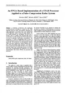
Figure 1: Hardware architecture for computing dotproducts. It consists of an array of 2M − 1 parallel multipliers followed by an adder reduction tree of depth ⌈log2 (2M − 1)⌉. The rest of the operations in a MINRES iteration use dedicated components. Independent memories are used to hold columns of the stored matrix Ak (refer to Section 5.6 for more details). z −M denotes a delay of M cycles. re-ordering, matrix Ak becomes banded (refer to Figure 4) and symmetric but indefinite, hence has both positive and negative eigenvalues. The size and half-bandwidth of Ak in terms of the control problem parameters are given respectively by N
:=
T (2n + m) + 2n,
(5a)
M
:=
2n + m.
(5b)
Notice that the number of outputs p and the number of constraints l does not affect the size of Ak , which we will show to determine the total runtime. This is another important difference between our design and previous MPC implementations. The minimum residual (MINRES) method is a suitable iterative algorithm for solving linear systems with indefinite symmetric matrices [7]. At each MINRES iteration, a matrixvector multiplication accounts for the majority of the computations. This kind of operation is easy to parallelize and consists of multiply-accumulate instructions, which are known to map efficiently into hardware in terms of resources. In [4] the authors propose an FPGA implementation for solving this type of linear systems using the MINRES method, reporting speed-ups of around one order of magnitude over software implementations. Most of the acceleration is achieved through a deeply pipelined dedicated hardware block (shown in Figure 1) that parallelizes dot-product operations for computing the matrix-vector multiplication in a row-by-row fashion. We use this architecture in our design with a few modifications to customize it to the special characteristics of the matrices that arise in MPC. Notice that the size of the dotproducts that are computed in parallel is independent of the control horizon length T (refer to (5b)), thus computational resource usage does not scale with T . The remaining operations in the interior-point iteration are undertaken by a separate hardware block, which we call Stage 1. The resulting two-stage architecture is shown in Figure 2.
Figure 2: Proposed two-stage hardware architecture. Solid lines represent data flow and dashed lines represent control signals. Stage 1 performs all computations apart from solving the linear system. The input is the current state measurement x b and the output is the next optimal control move u∗0 (b x).
5.2
Pipelining
Since the linear solver will provide most of the acceleration by consuming most resources it is vital that it remains busy at all times. Hence, the parallelism in Stage 1 is chosen to be the smallest possible such that the linear solver is always active. Notice that if both blocks are to be doing useful work at all times, while the linear system for a specific problem is being solved, Stage 1 has to be updating the solution and linearizing for another independent problem. In addition, the architecture described in [4] has to process P independent problems simultaneously to match latency with throughput and make sure the dot product hardware is active at all times to achieve maximum efficiency. Hence, our design can process 2P independent QP problems simultaneously. The expression for P in terms of the matrix dimensions and the control problem parameters is given by ⌈ ⌉ 3N + 24⌈log2 (2M − 1)⌉ + 154 P := (6a) N ⌈ ⌉ 6(T + 1)n + 3T m + 24⌈log2 (4n + 2m − 1)⌉ + 154 = . (6b) 2(T + 1)n + T m For details on the derivation of (6a), refer to [4]; (6b) results from the formulation given in Section 4. The linear term results from the row by row processing for the matrix-vector multiplication (N dot-products) and serial-to-parallel conversions, whereas the log term comes from the depth of the adder reduction tree in the dot-product block. The constant term comes from the other operations in the MINRES iteration. It is important to note that P converges to a small number (P = 4) as the size of Ak increases, thus for large problems only 2P = 8 independent threads are required to fully utilize the hardware.
5.3
Sequential Block
When computing the coefficient matrix Ak , only the diagonal matrix Wk , defined in the Appendix, changes from one iteration to the next, thus the complexity of this calcula-
maximum latency to achieve a high clock frequency. Extra registers were added after the multiplier to match the latency of the adder for synchronization, as these are the most common operations. The latency of the divider is much larger (27 cycles) than the adder (12 cycles) and the multiplier (8 cycles), therefore it was decided not to mach the delay of the divider path, as it would reduce our flexibility for ordering computations. NOPs were inserted whenever division operations were needed, namely only when calculating Wk and s−1 k .
100
90
Floating point unit efficiency, %
80
70
60
Overall Linear Solver Stage 1
50
40 3
30
Comparison operations are also required for the line search method (Line 6 of Algorithm 1), however this is implemented by repeated comparison with zero, so only the sign bit needs to be checked and a full floating-point comparator is not needed.
20 2 10
0
0
5
10
15
20
25 30 Number of states, n
35
40
45
50
55
Figure 3: Floating point unit efficiency of the different blocks in the design and overall circuit efficiency with m = 3, p = 3, T = 20, and 20 line search iterations. Numbers on the plot represent the number of parallel instances of Stage 1 required to keep the linear solver active when more than one instance is required. tion is relatively small. If the structure of the problem is taken into account, we find that the remaining calculations in an interior-point iteration are all sparse and very simple compared to solving the linear system. Comparing the computational count of all the operations to be carried out in Stage 1 with the latency of the linear solver implementation, we come to the conclusion that for most control problems of interest (large problems with large horizon lengths), the optimum implementation of Stage 1 is sequential, as this will be enough to keep the linear solver busy at all times. This is a consequence of the latency of the linear solver being Θ(T 2 ) [4], whereas the number of operations in Stage 1 is only Θ(T ). As a consequence, Stage 1 will be idle most of the time for large problems. This is indeed the situation observed in Figure 3, where we have defined the floating point unit efficiency as floating point computations per iteration . #floating point units × cycles per iteration For very small problems it is possible that Stage 1 will take longer than solving the linear system. In this cases, in order to avoid having the linear solver idle, another instance of Stage 1 is synthesized to operate in parallel with the original instance and share the same control block. For large problems, only one instance of Stage 1 is required. The efficiency of the circuit increases as the problems become larger as a result of the dot-product block, which is always active by design, consuming a greater portion of the overall resources.
5.3.1 Datapath The computational block performs any of the main arithmetic operations: addition/subtraction, multiplication and division. Xilinx Core Generator [1] was used to generate highly optimized single-precision floating point units with
The total number of floating point units in the circuit is given by Number of Floating Point Units = 8n + 4m + 27,
(7)
where only three units belong to Stage 1, which explains the behaviour observed in Figure 3.
5.3.2
Control Block
Since the same computational units are being reused to perform many different operations, the necessary control is rather complex. The control block needs to provide the correct sequence of read and write addresses for the data RAMs, as well as other control signals, such as computation selection. An option would be to store the values for all control signals at every cycle in a program memory and have a counter iterating through them. However, this would take a large amount of memory. For this reason it was decided to trade a small increase in computational resources for a much larger decrease in memory requirements. Frequently occurring memory access patterns have been identified and a dedicated address generator hardware block has been built to generate them from minimum storage. Each pattern is associated with a control instruction. Examples of these patterns are: simple increments a, a+1, ..., a+b and the more complicated read patterns needed for matrix vector multiplication (standard and transposed). This approach allows storing only one instruction for a whole matrix-vector multiplication or for an arbitrary long sequence of additions. Control instructions to perform line search and linearization for one problem were stored. When the last instruction is reached, the counter goes back to instruction 0 and iterates again for the next problem with the necessary offsets being added to the control signals.
5.3.3
Memory Subsystem
Separate memory blocks were used for data and control instructions, allowing simultaneous access and different wordlengths in a similar way to a Harvard microprocessor architecture. However, in our circuit there are no cache misses and a useful result can be produced almost every cycle. The data memories are divided in two blocks, each one feeding one input of the computational block. The intermediate results can be stored in any of these simple dual-port RAMs for flexibility in ordering computations. The memory to store the control instructions is divided into four single port
ROMs corresponding to read and write addresses of each of the data RAMs. The responsibility for generating the remaining control signals is spread out over the four blocks.
5.4 Latency and Throughput Since the FPGA has completely predictable timing, we can calculate the latency and throughput of our system. For large problems, where the linear solver is busy at all times, the overall latency of the circuit will be given by Latency =
2IIP (P N + P )IM IN RES seconds, FPGAf req
(8)
where IM IN RES is the number of iterations the MINRES method takes to solve the linear system to the required accuracy, IIP is the number of outer iterations in the interiorpoint method (Algorithm 1), FPGAf req is the FPGA’s clock frequency, (P N + P ) is the latency of one MINRES iteration [4], and P is given by (6a). In that time the controller will be able to output the result to 2P problems.
5.5 Input/Output Stage 1 is responsible for handling the chip I/O. It reads the current state measurement x b as n 32-bit floating point values sequentially through a 32-bit parallel input data port. Outputting the m 32-bit values for the optimal control move u∗0 (b x) is handled in a similar fashion. When processing 2P problems, the average I/O requirements are given by 2P (32(n + m)) bits/second. Latency given by (8) For the example problems that we have considered in Section 6, the I/O requirements range from 0.2 to 10 kbits/second, which is well within any standard FPGA platform interface, such as PCI Express. The combination of a very computationally intensive task with very low I/O requirements, highlights the affinity of the FPGA for MPC computation.
5.6 Coefficient Matrix Storage When implementing an algorithm in software, a large amount of memory is available for storing intermediate results. In FPGAs, there is a very limited amount of fast on-chip memory, around 4.5MBytes for high-end memory-dense Xilinx Virtex-6 devices [2]. If a particular design requires more memory than available on chip, there are two negative consequences. Firstly, if the size of the problems we can process is limited by memory, it means that the computational capabilities of the device are not being fully exploited, since there will be unutilized slices and DSP blocks. Secondly, if we were to try to overcome this problem by using off-chip memory, the performance of the circuit is likely to suffer since off-chip memory accesses are slow compared to the on-chip clock frequency. By taking into account the special structure of the matrices that are fed to the linear solver in the context of MPC, we substantially reduce memory requirements so that this issue affects a smaller subset of problems. The matrix Ak is banded and symmetric (after re-ordering). On-chip buffering of these type of matrices using compressed diagonal storage (CDS) can achieve substantial memory savings with minimum control overhead in an FPGA implementation of the MINRES method [5]. The memory reductions are achieved by only storing the non-zero diagonals of
Figure 4: Structure of original and CDS matrices showing variables (black), constants (dark grey), zeros (white) and ones (light grey) for m = 2, n = 4, and T = 8.
the original matrix as columns of the new compressed matrix. Since the matrix is also symmetric, only the right hand side of the CDS matrix needs to be stored, as the left-hand columns are just delayed versions of the stored columns. In order to achieve the same result when multiplying by a vector, the vector has to be aligned with its corresponding matrix components. It turns out that this is simply achieved by shifting the vector by one position at every clock cycle, which is implemented by a serial-in parallel-out shift register (refer to Figure 1). The method described in [5] assumes a dense band; however, it is possible to achieve further memory savings by exploiting the structure of the MPC problem even further. The structure of the original matrix and corresponding CDS matrix for a small MPC problem are shown in Figure 4, showing variables (elements that can vary from iteration to iteration of the interior-point method) and constants. The first observation is that non-zero blocks are separated by layers of zeros in the CDS matrix. It is possible to only store one of these zeros per column and add common circuitry to generate appropriate sequences of read addresses, i.e. 0, 0, ..., 0, 1, 2, ..., m+n, 0, 0, ..., 0, m+n+1, m+n+2, ..., 2(m+n) The second observation is that only a few diagonals adjacent to the main diagonal vary from iteration to iteration, while the rest remain constant at all times. This means that only a few columns in the CDS matrix contain varying elements. This has important implications, since in the MINRES implementation [4], matrices for the P problems that are being processed simultaneously have to be buffered on-chip. These memory blocks have to be double in size to allow writing the data for the next problems while reading the data for the current problems. Constant columns in the CDS matrix are common for all problems, hence the memories used to store them can be much smaller. Finally, constant columns mainly consist of repeated blocks of size 2n + m (where n values are zeros or ones), hence further memory savings can
9
100
10
8
dense banded symmetric (CDS) MPC (CDS) Virtex6 VSX 475T
90 registers LUTs BlockRAMs DSP48s
80
10
Resource usage, %
Memory requirements, bits
70 7
10
6
10
60
50
40
30
5
20
10
10
0
4
10 0 10
1
10 Number of states, n
Figure 5: Memory requirements for storing the coefficient matrices under different schemes. Problem parameters are m = 3 and T = 20. p and l do not affect the memory requirements of Ak . The horizontal line represents the memory available in a memorydense Virtex 6 device [2].
be attained by only storing one of those blocks per column. A memory controller for the variable columns and another memory controller for the constant columns were created in order to be able to generate the necessary access patterns. The impact on the overall performance is negligible, since these controllers consume few resources compared with floating point units and they do not slow down the circuit. If we consider a dense band, storing the coefficient matrix using CDS would require 2P (T (2n + m) + 2n)(2n + m) elements. By taking into account the sparsity of matrices arising in MPC, it is possible to only store 2P (1 + T (m + n) + n)n + (1 + m + n)(m + n) elements. Figure 5 compares the memory requirements for storing the coefficient matrices on-chip when considering: a dense matrix, a banded symmetric matrix and an MPC matrix (all in single-precision floating-point). Memory savings of approximately 75% can be incurred by considering the in-band structure of the MPC problem compared to the standard CDS implementation. In practice, columns are stored in BlockRAMs of discrete sizes, therefore actual savings vary in the FPGA implementation.
6. RESULTS 6.1 Resource Usage The design was synthesized using Xilinx XST and placed and routed using Xilinx ISE 12 targeting a Virtex 6 VSX 475T [2]. Figure 6 shows how the different resources scale with the problem size. For m and T fixed, the number of floating point units is Θ(n), hence the linear growth in registers, look-up tables and embedded DSP blocks. The memory requirements are Θ(n2 ), which explain the quadratic asymptotic growth observed in Figure 6. The jumps occur when the number of elements to be stored in the RAMs for variable columns exceeds the size of Xilinx BlockRAMs. If the
10
15
20
25
30 35 Number of states, n
40
45
50
55
Figure 6: Resource utilization on a Virtex 6 VSX 475T (m = 3, T = 20, P given by (6a)). number of QP problems being processed simultaneously is chosen smaller than the value given by (6a), the BlockRAM usage will decrease, whereas the other resources will remain unaffected.
6.2
Performance
Post place-and-route results showed that a clock frequency above 150MHz is achievable with very small variations for different problem sizes, since the critical path is inside the control block in Stage 1. Figure 7 shows the latency and throughput performance of the FPGA and latency results for a microprocessor implementation. For the software benchmark, we have used a direct C sequential implementation, compiled using GCC -O4 optimizations running on a Intel Core2 Q8300 with 3GB of RAM, 4MB L2 cache, and a clock frequency of 2.5GHz running Linux. Note that for matrix operations of this size, this approach produces better performance software than using libraries such as Intel MKL. As expected, the microprocessor performance is far from its peak for smaller problems, since the algorithm involves lots of movements of small blocks of data to exploit structure, specially for the operations outside the linear solver. Figure 7 shows how the performance gap between the CPU and FPGA widens as the size of the problem increases as a result of increased parallelism in the linear solver. Approximately a 6.5x improvement in latency and a 51x improvement in throughput are possible for the largest problem considered. However, notice that even for large problems there is a large portion of unutilized resources, which could be used to extract more parallelism in the interior-point method and achieve even greater speed-ups.
7.
CASE STUDY
To illustrate the performance improvement that can be achieved with the sampling frequency upgrade enabled by our FPGA implementation, we apply our MPC controller to an example system under different sampling intervals. The example system consists of 16 masses connected by equal springs (shown in Figure 8). Mass number three is eight times lighter than
1
10
Table 3: Computational delay for each implementation when IIP = 14. In MPC, the computational delay has to be smaller than the sampling interval. The grey region represents cases where the computational delay is larger than the sampling interval, hence the implementation is infeasible. The smallest sampling interval that the FPGA can handle is 0.388 seconds (2.58Hz), whereas the CPU samples every 0.775 seconds (1.29Hz). The relationship T s = TTh holds. T FPGA CPU Sampling interval, Ts 4 0.110 0.503 0.775 5 0.161 0.721 0.620 6 0.221 0.995 0.517 7 0.291 1.291 0.442 8 0.371 1.641 0.388 9 0.460 2.023 0.344
CPUmeasured FPGA1
0
10
FPGA
Time per interior−point iteration
full
−1
10
−2
10
−3
10
−4
10
0
1
10
10 Number of states, n
Figure 7: Performance comparison showing measured performance of the CPU, and FPGA performance when solving one problem and 2P problems given by (6a). Problem parameters are m = 3, T = 20, p = 3, and FPGAf req = 150MHz. y2
M1 u1
Output 3
yp
M2 u2
Mp
This paper has described a parameterizable FPGA architecture for solving QP optimization problems in linear MPC. Various design decisions have been justified based on the
5
10
15
0
5
10
15
0
5
10
15
0
3000
Cost
8. CONCLUSION
0
−0.5
Figure 8: Spring-mass system.
The control horizon length (Th ) for a specific system is specified in seconds, therefore, sampling faster leads to more steps in the horizon (T ) and larger optimization problems to solve at each sampling instant. For the example system we found that this quantity was approximately Th = 3.1 seconds. Table 3 shows the sampling interval and computational delays for the CPU and FPGA implementations for different number of steps in the horizon. For each implementation, the operating sampling interval is chosen the smallest possible such that the computational delay allows solving the optimization problem before the next sample needs to be taken. Figure 9 presents the simulation results, which highlight the better tracking achievable with the FPGA implementation, leading to lower control cost. Notice the terrible response of the CPU implementation after the disturbance takes place, whereas the FPGA response is oscillation absent.
0
0.5
um
the other masses, which results in an oscillatory mode at 0.66Hz. There are two states per mass, its position and velocity, hence the system has 32 states. Each mass can be actuated by a horizontal force (m = 16) and the reference for the outputs to track is the zero position for all masses (p = 16).
2
−2
Input 3
y1
4
2000 1000 0
Time, seconds
Figure 9: Comparison of the closed-loop performance of the FPGA (solid) and the CPU (dashed). The dotted lines represent the physical constraints of the system. The simulation includes a disturbance on the inputs between 7 and 8 seconds.
significant exploitable structure in the problem. The main source of acceleration is a parallel linear solver block, which reduces the latency of the main computational bottleneck in the optimization method. Results show that a significant reduction in latency is possible compared to a sequential software implementation, which translates to high sampling frequencies and better quality control. The potential for industrial take-up of this technology is currently being explored with our partners. We are currently working on completely automating the design flow with the objective of choosing the data representation and level of parallelism that makes the most efficient use of all resources available in any given target FPGA platform, avoiding the situation observed in Figure 6, where for a large number of states, memory resources are exhausted well before logic resources.
9. ACKNOWLEDGMENTS The authors would like to acknowledge the support of the EPSRC (Grant EP/G031576/1), discussions with Prof. Jan Maciejowski, Prof. Ling Keck Voon, Mr. David Boland and Mr. Amir Shazhad, and industrial support from Xilinx, the Mathworks, and the European Space Agency.
[15]
[16]
10. REFERENCES [1] Core Generator guide, 2010 http://www.xilinx.com/itp/xilinx6/books/docs/cgn/ cgn.pdf. [2] Virtex-6 family overview, 2010 http://www.xilinx.com/support/documentation/ data sheets/ds150.pdf. [3] S. Bayliss, C. S. Bouganis, and G. A. Constantinides. An FPGA implementation of the Simplex algorithm. In Proc. Int. Conf. on Field Programmable Technology, pages 49–55, Bangkok, Thailand, Dec 2006. [4] D. Boland and G. A. Constantinides. An FPGA-based implementation of the MINRES algorithm. In Proc. Int. Conf. on Field Programmable Logic and Applications, pages 379–384, Heidelberg, Germany, Sep 2008. [5] D. Boland and G. A. Constantinides. Optimising memory bandwidth use for matrix-vector multiplication in iterative methods. In Proc. Int. Symp. on Applied Reconfigurable Computing, pages 169–181, Bangkok, Thailand, Mar 2010. [6] S. P. Boyd and L. Vandenberghe. Convex Optimization. Cambridge University Press, Cambridge, UK, 2004. [7] B. Fisher. Polynomial based iteration methods for symmetric linear systems. Wiley, Baltimore, MD, USA, 1996. [8] T. A. Johansen, W. Jackson, and P. T. Robert Schreiber. Hardware synthesis of explicit model predictive controllers. IEEE Transactions on Control Systems Technolog, 15(1):191–197, Jan 2007. [9] T. Keviczky and G. J. Balas. Receding horizon control of an F-16 aircraft: A comparative study. Control Engineering Practice, 14(9):1023–1033, Sep 2006. [10] G. Knagge, A. Wills, A. Mills, and B. Ninnes. ASIC and FPGA implementation strategies for model predictive control. In Proc. European Control Conference, Budapest, Hungary, Aug 2009. [11] S. L. Koh. Solving interior point method on a FPGA. Master’s thesis, Nanyang Technological University, Singapore, 2009. [12] M. S. Lau, S. P. Yue, K.-V. Ling, and J. M. Maciejowski. A comparison of interior point and active set methods for FPGA implementation of model predictive control. In Proc. European Control Conference, pages 156–160, Budapest, Hungary, Aug 2009. [13] B. Leung, C.-H. Wu, S. O. Memik, and S. Mehrotra. An interior point optimization solver for real time inter-frame collision detection: Exploring resource-accuracy-platform tradeoffs. In Proc. Int. Conf. on Field Programmable Logic and Applications, pages 113–118, Milano, Italy, Sep 2010. [14] K.-V. Ling, B. F. Wu, and J. M. Maciejowski. Embedded model predictive control (MPC) using a
[17] [18]
[19] [20]
[21]
[22]
FPGA. In Proc. 17th IFAC World Congress, pages 15250–15255, Seoul, Korea, Jul 2008. K.-V. Ling, S. P. Yue, and J. M. Maciejowski. An FPGA implementation of model predictive control. In Proc. American Control Conference, page 6 pp., Minneapolis, USA, Jun 2006. A. R. Lopes and G. A. Constantinides. A high throughput FPGA-based floating-point conjugate gradient implementation for dense matrices. In Proc. 4th Int. Workshop on Applied Reconfigurable Computing, pages 75–86, London, UK, Mar 2008. J. Maciejowski. Predictive Control with Constraints. Pearson Education, Harlow, UK, 2001. S. Mehrotra. On the implementation of a primal-dual interior point method. SIAM Journal on Optimization, 2(4):575–601, Nov 1992. J. Nocedal and S. J. Wright. Numerical Optimization. Springer, New York, USA, 2006. P. D. Vouzis, L. G. Bleris, M. G. Arnold, and M. V. Kothare. A system-on-a-chip implementation for embedded real-time model predictive control. IEEE Transactions on Control Systems Technology, 17(5):1006–1017, Sep 2009. S. J. Wright. Applying new optimization algorithms to model predictive control. In Proc. Int. Conf. Chemical Process Control, pages 147–155. CACHE Publications, 1997. S. J. Wright. Primal-Dual Interior-Point Methods. SIAM, Philadelphia, USA, 1997.
APPENDIX This appendix provides the remaining details of the QP algorithm, removed from the pseudo-code in Algorithm 1 for readability. In the following, σ is a scalar between zero and one known as the centrality parameter [21], and Λk and Sk are diagonal matrices containing the elements of λk and sk respectively. Wk := Λk Sk−1 µk :=
λ′k sk T l + 2p
rkθ := −(H + G′ Wk G)θk − F ′ νk − G′ (λk − Wk g + σµk s−1 k ) rkν := −F θk + f ∆λk := Wk (G(θk + ∆θk ) − g) + σµk s−1 k ∆sk := −sk − (G(θk + ∆θk ) − g)