RIKEN BSI BSIS Technical Report No.02-5
1
Blind Gene Classification - An ICA-based Gene Classification/Clustering Method Gen Hori1∗, Masato Inoue2,3 , Shin-ichi Nishimura2,4 and Hiroyuki Nakahara2 1 Laboratory for Advanced Brain Signal Processing, Brain Science Institute, RIKEN, Saitama 351-0198, Japan 2 Laboratory for Mathematical Neuroscience, Brain Science Institute, RIKEN, Saitama 351-0198, Japan 3 Department of Otolaryngology, Graduate School of Medicine, Kyoto University, Kyoto 606-8507, Japan 4 Department of Otolaryngology, Faculty of Medicine, University of Tokyo, Tokyo 113-8656, Japan {hori@bsp.,minoue@,nishi@mns.,hiro@}brain.riken.go.jp
Keywords: gene expression data, independent component analysis (ICA), gene classification/clustering Abstract Motivation: To develop a gene classification method exploiting statistical structure of gene expression data, we apply independent component analysis (ICA) to microarray data. Results: We introduce an ICA-based gene classification method. By using a gene expression data of yeast during sporulation, we validate our classification method. The ICA-based method automatically finds typical gene profiles, which are similar to average profiles of biologically meaningful gene groups, and classifies the yeast genes based on the obtained typical profiles. Contact:
[email protected]
1
Introduction
Gene classification/clustering is one of the central issues in gene expression data analysis because it is extremely useful to classify or cluster the enormous number of genes into relatively small number of groups to draw valuable information from the data. For that ∗
To whom correspondence should be addressed.
RIKEN BSI BSIS Technical Report No.02-5
2
purpose, many works have been made on applying known unsupervised learning methods, such as hierarchical clustering (Eisen et al., 1998) and self-organizing maps (Tamayo et al., 1999), to gene classification problem. We previously proposed to apply independent component analysis (ICA; Cardoso and Souloumiac, 1993; Bell and Sejnowski, 1995; Hyvaerinen and Oja, 1997; Amari et al., 1997) to gene expression data and pointed out that ICA automatically finds the typical gene profiles from gene expression data and classifies genes successfully into biologically suitable groups using the obtained typical profiles (Hori et al., 2001). Also Liebermeister applied ICA to gene expression data to find independent modes of gene expression (Liebermeister, 2002). The present study introduces a scheme of ICA-based analysis in gene expression data analysis and extends our former ICA-based gene classification method. The organization of the rest of the paper is as follows. Section 2 gives a brief introduction to independent component analysis (ICA), discusses how to apply ICA to a gene expression data and introduces linear profile model and our gene classification method. Section 3 validates our methods using a publicly accessible yeast gene expression data, by comparing the model profiles and the classification results by ICA to the average profiles of biologically meaningful gene groups and the classification result based on them respectively. Discussion follows in Section 4.
2 2.1
Methods Independent component analysis (ICA)
Independent component analysis (ICA) is a method for multi-channel signal processing to separate mixed signals. Methods for the signals mixed with and without time delay are also called blind source deconvolution (BSD) and blind source separation (BSS) respectively, and the ICA algorithm applied to microarray data in the following belongs to the latter. ICA has advantage to PCA in that the former exploits higher order statistics and has no restriction on its transformation, whereas the latter exploits only second order statistics and is restricted to orthogonal transformation. ICA has been well established and successfully applied to analyze brain signals, such as EEG, MEG and MRI, and also speech signals and images. ICA for the signals mixed without time delay is based on the mixing model x(t) = As(t),
t = 1, . . . , m
(1)
y(t) = W x(t),
t = 1, . . . , m
(2)
and the demixing model where s(t) = (s1 (t), . . . , sn (t))T , x(t) = (x1 (t), . . . , xn (t))T and y(t) = (y1 (t), . . . , yn (t))T denote the source signals, the mixed signals and the demixed signals respectively, and A and W denote the n × n mixing and demixing matrix respectively. The mixing and demixing models are written in the matrix forms as X = AS and Y = W X where S, X
RIKEN BSI BSIS Technical Report No.02-5
3
and Y denote the n × m matrices whose t-th columns are s(t), x(t) and y(t) respectively (Figure 1).
ICA assumes that the source signals s(t) are zero-mean, E[si (t)] = 0,
i = 1, . . . , n,
and independent to each other, that is, the joint probability distribution of the source signals are the product of non-Gaussian marginal distributions, p(s1 , s2 , . . . , sn ) = p(s1 )p(s2 ) · · · p(sn ). Here we should note that only the mixed signals x(t) are observable and the source signals s(t) and the mixing matrix A are not. Also only the zero-mean, independence and nonGaussian assumptions are all the available information on the source signals s(t) and their probability distributions are unknown. The zero-mean assumption of the source signals is not a matter for applying ICA to gene expression data because it can be circumvented by removing means from observed mixed signals x(t) before applying ICA and restoring them after the demixing matrix is obtained. ICA attempts to find the demixing matrix W such that the demixed signals y(t) are close to the source signals s(t) as possible, exploiting the independence assumption on the source signals s(t). Although the ideal solution is W = A−1 , ICA finds this inverse except the indeterminacy of the permutation and the amplitude of its rows. An ICA algorithm is an updating rule of the demixing matrix W which minimizes some criterion of the dependency, for example mutual information, between the observed signals y(t). Starting from some appropriate initial matrix, such an updating rule makes W converge to the inverse except the above indeterminacy. We use the JADE algorithm (Cardoso and Souloumiac, 1993), an ICA algorithm based on the joint diagonalization (Bunse et al., 1993; Hori, 2000) of the fourth order cumulant tensor of the prewhitened observed signals, for our ICA analysis of gene expression data.
2.2
Demixing model for gene expression data
This section discusses a feasible way of applying ICA to a gene expression data and the interpretation of the corresponding mixing model. Let X denote a matrix of gene expression data with m rows of genes and n columns of conditions and xij the (i, j)-th element of the matrix X which corresponds to the i-th
RIKEN BSI BSIS Technical Report No.02-5
4
gene’s expression ratio under the j-th condition. In most cases, the number of genes m is much larger than the number of conditions of experiment n. Hence we employ the demixing model (3) ST = W XT , where T denotes matrix transpose and W is an n × n demixing matrix. By this demixing model, we can make the estimation of the demixing matrix feasible. The demixing model (3) takes the rows of X as m observations of an n-dimensional variable. Once the demixing matrix W and S T are obtained by ICA, the gene expression data X T is calculated inversely from S T as X T = AS T (4) where A = W −1 denotes the inverse of the demixing matrix (Figure 2).
When we employ the demixing model (3), the corresponding mixing model (4) can be understood as follows. We suppose that there are n controlling factors, which are statistically independent to each other, underlying in gene expression. The rows and columns of the mixing matrix A correspond to the experiment conditions and the controlling factors respectively. The (j, k)-th element ajk of A represents the amount of the k-th controlling factor under the j-th condition. On the other hand, the rows and columns of the matrix S T correspond to the controlling factors and the genes respectively. The (k, i)-th element of S T represents the contribution of the k-th controlling factor to the i-th gene’s expression. Then the expression of the i-th gene under j-th condition represented in the (i, j)-th element xij of X is calculated as the sum of the amount of the controlling factors ajk weighted by the contributions sik . Let us remind that the rows of the obtained demixing matrix W have the indeterminacy of amplitude and permutation in the framework of ICA. To make the demixing model (3) and the mixing model (4) uniquely determined, hence we suppose in the following that the rows of S T are normalized to have unit variance, the columns of A are sorted in descending order with respect to their Euclidean norms and the signs of the columns of A are chosen so that their means become positive values.
2.3
Linear profile model
This section proposes the linear profile model in which each of all the gene profiles in expression data is expressed in the linear combinations of a few model profiles (see below) obtained by ICA. We will see in Section 3 that the model profiles have consistency with
RIKEN BSI BSIS Technical Report No.02-5
5
the average profiles of biologically meaningful gene groups and the linear profile model is a powerful tool for investigating how a gene expression data are organized and classifying or clustering genes into biologically suitable groups. The relation of mixing (4) is written column-wise as x(t) = As(t),
t = 1, . . . , m
(5)
where x(t) and s(t) denote the t-th columns of X T and S T respectively. The column vector x(t) contains the t-th gene’s profile. The column-wise relation (5) can be read as an expansion of the t-th gene’s profile vector with the basis vectors ak (k = 1, . . . , n) representing the k-th columns of the matrix A and the basis coefficients sk (t) representing the k-th component of s(t), x(t) =
n X
sk (t)ak .
(6)
k=1
We refer to the basis vectors ak (k = 1, . . . , n) as model profiles and the relation (6) that represents all the gene profiles in the linear combinations of the model profiles as linear profile model (Figure 3). The k-th model profile ak can be regarded as the profile of a gene which is contributed only by the k-th controlling factor and the linear profile model expresses the gene profiles in the linear combinations of model profiles weighted by the contributions of the controlling factors. Similarly to the relation of mixing (4), the relation of demixing (3) is written columnwise as s(t) = W x(t), t = 1, . . . , m (7) where W is the demixing matrix and s(t) and x(t) denote the t-th columns of S T and X T respectively. The column vector s(t) contains the contributions of the controlling factors to the t-th gene. The column-wise relation (7) can be also written as s(t) = (w1 · x(t), . . . , wn · x(t))T where the row vector wi is the i-th row of the demixing matrix W and w · x denotes the vector inner product of a row vector w and a column vector x. We refer to the row vectors w i (i = 1, . . . , n) as profile filters. The profile filters extract the contributions of the controlling factors from the gene profiles.
RIKEN BSI BSIS Technical Report No.02-5
6
Our framework of the linear profile model (6) corresponds to the framework of ‘feature extraction’ for natural images (Bell and Sejnowski, 1997). They applied ICA to natural scene images based on the linear image synthesis model (Olshausen and Field, 1996) where x(t) in (6) now denotes small patches from a natural image. The rows of the resulting demixing matrix W , corresponding to the receptive fields in early visual cortex of the brain, are found to be ‘edge filters’. The framework of ‘feature extraction’ has been successfully applied to image processing such as face recognition (Bartlett and Sejnowski, 1997) and lipreading (Gray et al., 1997). We note that the number of the model profiles in the framework described above is exactly the same as the number of the conditions of given gene expression data. The number of the model profiles can be reduced by i) applying ICA to the preprocessed data reconstructed from the top few principal components or ii) simply discarding the last model profiles obtained by ICA, which is sometimes good for eliminating ill influence from the weak components which might not capture essential information. On the other hand, the number of the model profiles can not be increased to exceed the number of the conditions of given gene expression data. Also we note that the model profiles obtained by ICA are basically not orthogonal to each other because, unlike PCA, ICA is not restricted to orthogonal transformation.
2.4
Blind gene classification
According to the framework of the linear profile model introduced in the previous section, it is reasonable to classify genes into groups associated with the controlling factors. Since each controlling factor is associated with a model profile, it is equivalent to classify genes into groups associated with the model profiles. This section introduces two generic gene classification scheme based on the obtained model profiles and the contributions of controlling factors respectively. Scheme I Scheme I classifies genes into groups associated with the model profiles according to some similarity measure between the gene profiles and the model profiles. Generically, each gene is classified into a group which shows the highest value of the similarity measure between the genes profile and the model profile. Specifically, we will use the correlation coefficient which is widely used similarity measure between gene profiles in the classification of yeast genes in Section 3.3. Scheme II Scheme II classifies genes into the groups activated and repressed by the controlling factors using the values of the elements of S T . We define a degree of gene’s sensitivity to the controlling factors by using the values of elements of S T . Generically, the genes with positive and negative extreme values of the degree of sensitivity are assigned to the activated and repressed group respectively. Specifically, we will simply use the value of
RIKEN BSI BSIS Technical Report No.02-5
7
sk (t) as the sensitivity of the t-th gene to the k-th controlling factor in the classification of yeast genes in Section 3.3. We refer to Scheme I and Scheme II as ‘blind gene classification’ or ‘blind classification/clustering’.
3
Results
The following sections validate our methods for understanding gene expression data and classifying genes using an actual gene expression data. Section 3.1 explains the yeast gene expression data we use for validation, Section 3.2 applies ICA to the data and investigates the obtained model profiles and the contributions of the controlling factors, and Section 3.3 shows the results of our gene classification methods.
3.1
Gene expression data for validation
We validate our method using a gene expression data of yeast during sporulation collected by Chu et al. (Chu et al., 1998) 1 . The data consists of expression data of 6118 genes in yeast genome which were measured at seven time points during sporulation, namely, 0.0, 0.5, 2.0, 5.0, 7.0, 9.0 and 11.5 hours. Chu et al. classified the yeast genes into seven groups based on the expression data using their domain knowledge. They hand-picked seven small sets of yeast genes, each of which consists of 3 - 8 representative genes of the respective time period. By averaging the profiles of each set over all the time periods, they defined seven average profiles in Figure 4. All the other yeast genes are then classified into one of the seven average profiles: Each gene is assigned to a group that shows the highest correlation coefficient between the average profile and the gene profile.
3.2
Obtained model profiles and controlling factors
Figure 5 shows the obtained model profiles, that is, the columns of the inverse of the obtained demixing matrix, A = W −1 . Notably, some model profiles in Figure 5 obtained automatically by ICA are similar to the average profiles in Figure 4 obtained manually by Chu et al. For example, IC1 , IC2 and IC3 in Figure 5 appear to match well with ‘Early I’, ‘Middle’ and ‘Mid-Late’ in Figure 4 respectively. Especially, the IC2 model profile is extremely similar to the ‘Middle’ average profile. This implies that the representative genes of the ‘Middle’ profile that Chu et al. hand-picked are directly related to the second controlling factor, which represents the second row of S T .
1
The data is available from http://cmgm.stanford.edu/pbrown/sporulation/.
RIKEN BSI BSIS Technical Report No.02-5
Figure 4
8
Average profiles manually obtained by Chu et al. (Chu et al., 1998)
Figure 5
Model profiles automatically obtained by ICA
The left and the right half of Figure 6 show the scatterplots (pairwise joint distributions) among the gene expressions xi (t) (i = 1, 2, . . . , 7) and among the contriubutions of controlling factors si (t) (i = 1, 2, . . . , 7) respectively. While ICA takes higher order relations into account for obtaining the demixing matrix, we can still make the following observation from the pairwise relations in the figure. There are some strongly correlated pairs in the scatterplots of the gene expressions, for example (x5 , x6 ) and (x6 , x7 ), whereas there are no such correlated pairs in the scatterplots of the contributions of controlling factors. This confirms that ICA extracts the underlying mutually independent controlling
RIKEN BSI BSIS Technical Report No.02-5
9
factors from the mutually dependent gene expression data. In the joint distributions between s2 and other si ’s (especially s1 , s4 and s6 ), there are jutting parts in which s2 takes large values while other si ’s are close to zero. These correspond to the genes whose profiles are very close to the model profile IC2 . There are similar jutting parts in some other pairwise joint distributions. Note that it is difficult to find these from the pairwise distributions of gene expressions xi (t) before applying ICA, as can been examined in the figure.
3.3
Classification resutls
According to the two classification scheme described in Section 2.4, the yeast genes are classified into seven groups associated with the obtained model profiles and controlling factors. We compare our two classification results with the classification by Chu et al. for evaluation of our method. In the following, for the sake of simple comparison, we make a representative group composed of the top 100 genes for each category instead of complete classification of all the genes. The results of the comparison are summarized in the table of the number of genes in the intersections between these groups. The representative groups are made as follows. For the average profiles defined by Chu et al. and the model profiles obtained by ICA, the genes with the top 100 highest correlation coefficients to categories of each profile are collected. For the controlling factors obtained by ICA, the genes with the top 100 highest contributions from the controlling factors are collected. Table 1 summarizes the number of genes in the intersections between
RIKEN BSI BSIS Technical Report No.02-5
10
these groups.
Metabolic Early I Early II Early-Mid Middle Mid-Late Late
IC1 14 42 0 0 0 0 0
Scheme I IC3 IC4 IC5 0 1 0 0 0 0 0 0 0 3 0 0 0 0 0 15 0 0 0 0 0
IC2 0 0 0 20 78 1 0
Table 1
IC6 0 0 0 0 0 0 0
IC7 6 0 0 0 0 0 0
IC1 13 28 8 6 1 0 0
IC2 0 1 1 8 55 2 1
Scheme II IC3 IC4 IC5 0 2 2 1 2 0 0 0 2 6 0 0 3 0 3 18 0 0 2 0 0
IC6 0 1 1 0 0 1 0
IC7 0 0 0 0 3 2 1
Numbers of genes in the intersections
From the above results, we find three correspondence between the model profiles obtained by ICA and the average profiles of Chu et al., namely, IC1 , IC2 and IC3 between ‘Early’ ‘Middle’ and ‘Mid-Late. These correspondence are the same as we observed from the shapes of the profiles in the last section. From these, we conclude that the three of the model profiles or controlling factors obtained by ICA automatically capture some feature of the yeast gene expression data. On the other hand, the rest of model profiles have no obvious correspondence to the average profiles. It is not clear if they capture some other feature of the expression data the average profiles do not capture.
4
Discussion
Using the yeast gene expression data during sporulation, we have validated our linear profile model and blind gene classification method. ICA automatically discovered three model profiles that are similar to three of the average profiles manually obtained by Chu et al. Especially, the IC2 model profile was very similar to the ‘Middle’ average profile. The top 10 genes activated by the second controlling factor include DIT1, SPR28, SSP1 and SPR3 that are related to spore wall formation whereas the top 10 genes repressed by the second controlling factor include MEP2, ERG6, ACS2 and IDH1 that are related to metabolism. Let us briefly discuss limitations and future works of the present study. First, in the present study, we implemented the simplest cases of the classification methods of both Scheme I and Scheme II introduced in Section 2.4. It is worthwhile to consider more sophisticated cases using other measures of similarity of profiles or contributions of controlling factors. Second, the present study examined only the activated groups of Scheme II, simply because they are easy to be compared to the classification result using the average profiles. The corresponding repressed groups are also of interest. Third, it is interesting to combine our ICA-generated model profiles with other gene classification methods such as hierarchical clustering or tree harvesting.
RIKEN BSI BSIS Technical Report No.02-5
11
References Amari,S., Chen,T.-P. and Cichocki,A. (1997) Stability analysis of adaptive blind source separation. Neural Networks, 10(8), 1345-1352. Bartlett,M. and Sejnowski,T.J. (1997) Viewpoint invariant face recognition using independent component analysis and attractor networks. In Advances in Neural Information Processing Systems, MIT Press, 9, 817-823. Bell,A.J. and Sejnowski,T.J. (1995) An information-maximization approach to blind separation and blind deconvolution. Neural Computation, 7, 1129-1159. Bell,A.J. and Sejnowski,T.J. (1997) The ’independent components’ of natural scenes are edge filters. Vision Research, 37(23), 3327-3338. Bunse-Gerstner,A., Byers,R. and Mehrmann,V. (1993) Numerical methods for simultaneous diagonalization. SIAM J. Mat. Anal. Appl., 14, 927-949. Cardoso,J.-F. and Souloumiac,A. (1993) Blind beamforming for non Gaussian signals. IEEE Proc.-F, 140, 362-370. Chu,S., DeRisi,J., Eisen,M., Mulholland,J., Botstein,D., Brown,P.O. and Herskowitz,I. (1998) The transcriptional program of sporulation in budding yeast. Science, 282, 699705. Eisen,M.B., Spellman,P.T., Brown,P.O. and Botstein,D. (1998) Cluster analysis and display of genome-wide expression patterns. Proc. Natl. Acad. Sci. USA, 95(25), 1486314868. Gray,M.S., Movellan,J.R. and Sejnowski,T.J. (1997) A comparison of local versusglobal image decompositions for visual speechreading. Proc. 4th Joint Symposium on Neural Computation, 92-98 Hori,G. (2000) A new approach to joint diagonalization. Proc. 2nd Int. Workshop on Independent Component Analysis and Blind Signal Separation (ICA2000), Helsinki, Finland, 151-155. Hori,G., Inoue,M., Nishimura,S. and Nakahara,H. (2001) Blind gene classification based on ICA of microarray data. Proc. 3rd Int. Workshop on Independent Component Analysis and Blind Signal Separation (ICA2001), SanDiego, U.S.A., 332-336. Hori,G., Inoue,M., Nishimura,S. and Nakahara,H. (2001) Blind gene classification — an ap-
RIKEN BSI BSIS Technical Report No.02-5
12
plication of a signal separation method. Proc. Genome Informatics Workshop (GIW2001), Tokyo, Japan, 255-256. Hyvaerinen,A. and Oja,E. (1997) A fast fixed-point algorithm for independent component analysis. Neural Computation, 9, 1483-1492. Liebermeister,W. (2002) Linear modes of gene expression determined by independent component analysis. Bioinformatics, 18(1), 51-60. Olshausen,B. and Field,D. (1996) Emergence of simple-cell receptive field properties by lerning a sparse code for natural images. Nature, 381, 607-609. Raychaudhuri,S., Stuart,J.M. and Altman,R.B. (2000) Principal component analysis to summarize microarray experiments: application to sporulation time series. Pacific Symposium on Biocomputing, 5, 452-463. Tamayo,P., Slonim,D., Mesirov,J., Zhu,Q., Kitareewan,S., Dmitrovsky,E., Lander,E.S. and Golub,T.R. (1999) Interpreting patterns of gene expression with self-organizing maps: methods and application to hematopoietic differentiation. Proc. Natl. Acad. Sci. USA, 96(6), 2907-2912.