to Computer Security. By. Steven Andrew Hofmeyr. B.Sc. (Hons), Computer Science, University of the Witwatersrand, 1991. M.Sc., Computer Science, University ...
An Immunological Model of Distributed Detection and Its Application to Computer Security By
Steven Andrew Hofmeyr B.Sc. (Hons), Computer Science, University of the Witwatersrand, 1991 M.Sc., Computer Science, University of the Witwatersrand, 1994
Doctor of Philosophy Computer Science
May 1999
c 1999, Steven Andrew Hofmeyr
iii
Dedication
To the Babs for having such patience when I was so far away, and to my dearest Folks for getting me this far.
v
Acknowledgments
The author gratefully acknowledges the help of the following people: D. Ackley, P. D’haeseleer, S. Forrest, G. Hunsicker, S. Janes, T. Kaplan, J. Kephart, B. Maccabe, M. Oprea, B. Patel, A. Perelson, D. Smith, A. Somayaji, G. Spafford, and all the people in the Adaptive Computation Group at the University of New Mexico. This research was supported by the Defense Advanced Research Projects Agency (grant N00014-961-0680) the National Science Foundation (grant IRI-9711199), the Office of Naval Research (grant N0001499-1-0417), the IBM Partnership award, and the Intel Corporation. S TEVEN H OFMEYR
The University of New Mexico May 1999
vii
An Immunological Model of Distributed Detection and Its Application to Computer Security By
Steven Andrew Hofmeyr
Doctor of Philosophy Computer Science
May 1999
An Immunological Model of Distributed Detection and Its Application to Computer Security by
Steven Andrew Hofmeyr B.Sc. (Hons), Computer Science, University of the Witwatersrand, 1991 M.Sc., Computer Science, University of the Witwatersrand, 1994 Ph.D., Computer Science, University of New Mexico, 1999
Abstract This dissertation explores an immunological model of distributed detection, called negative detection, and studies its performance in the domain of intrusion detection on computer networks. The goal of the detection system is to distinguish between illegitimate behaviour (nonself ), and legitimate behaviour (self ). The detection system consists of sets of negative detectors that detect instances of nonself; these detectors are distributed across multiple locations. The negative detection model was developed previously; this research extends that previous work in several ways. Firstly, analyses are derived for the negative detection model. In particular, a framework for explicitly incorporating distribution is developed, and is used to demonstrate that negative detection is both scalable and robust. Furthermore, it is shown that any scalable distributed detection system that requires communication (memory sharing) is always less robust than a system that does not require communication (such as negative detection). In addition to exploring the framework, algorithms are developed for determining whether a nonself instance is an undetectable hole, and for predicting performance when the system is trained on nonrandom data sets. Finally, theory is derived for predicting false positives in the case when the training set does not include all of self. Secondly, several extensions to the model of distributed detection are described and analysed. These extensions include: multiple representations to overcome holes; activation thresholds and sensitivity levels to reduce false positive rates; costimulation by a human operator to eliminate autoreactive detectors; distributed detector generation to adapt to changing self sets; dynamic detectors to avoid consistent gaps in detection coverage; and memory, to implement signature-based detection. Thirdly, the model is applied to network intrusion detection. The system monitors TCP traffic in a broadcast local area network. The results of empirical testing of the model demonstrate that the system detects real intrusions, with false positive rates of less than one per day, using at most five kilobytes per computer. The system is tunable, so detection rates can be traded off against false positives and resource usage. The system detects new intrusive behaviours (anomaly detection), and exploits knowledge of past intrusions to improve subsequent detection (signature-based detection).
xi
Contents List of Figures
xvi
List of Tables
xviii
Glossary of Symbols 1
2
3
xix
Introduction 1.1 Immunology . . . . . . . . . . . . . . . . 1.2 Computer Security . . . . . . . . . . . . . 1.3 Principles for an Artificial Immune System 1.4 The Contributions of this Dissertation . . . 1.5 The Remainder of this Dissertation . . . .
. . . . .
. . . . .
. . . . .
. . . . .
. . . . .
. . . . .
. . . . .
. . . . .
. . . . .
. . . . .
. . . . .
. . . . .
. . . . .
. . . . .
. . . . .
. . . . .
. . . . .
. . . . .
. . . . .
. . . . .
Background 2.1 Immunology for Computer Scientists . . . . . . . . . . . . . . . . . . . . . . . 2.1.1 Recognition . . . . . . . . . . . . . . . . . . . . . . . . . . . . . . . 2.1.2 Receptor Diversity . . . . . . . . . . . . . . . . . . . . . . . . . . . . 2.1.3 Adaptation . . . . . . . . . . . . . . . . . . . . . . . . . . . . . . . . 2.1.4 Tolerance . . . . . . . . . . . . . . . . . . . . . . . . . . . . . . . . . 2.1.5 MHC and diversity . . . . . . . . . . . . . . . . . . . . . . . . . . . . 2.2 A First Attempt at Applying Immunology to ID: Host-based Anomaly Detection 2.3 Network Intrusion Detection . . . . . . . . . . . . . . . . . . . . . . . . . . . 2.3.1 Networking and Network Protocols . . . . . . . . . . . . . . . . . . . 2.3.2 Network Attacks . . . . . . . . . . . . . . . . . . . . . . . . . . . . . 2.3.3 A Survey of Network Intrusion Detection Systems . . . . . . . . . . . 2.3.4 Building on Network Security Monitor . . . . . . . . . . . . . . . . . 2.3.5 Desirable Extensions to NSM . . . . . . . . . . . . . . . . . . . . . . 2.4 An Immunologically-Inspired Distributed Detection System . . . . . . . . . . . An Immunological Model of Distributed Detection 3.1 Properties of The Model . . . . . . . . . . . . 3.1.1 Problem Description . . . . . . . . . 3.1.2 Distributing the Detection System . . 3.1.3 Assumptions . . . . . . . . . . . . . 3.1.4 Generalization . . . . . . . . . . . . 3.1.5 Scalable Distributed Detection . . .
xiii
. . . . . .
. . . . . .
. . . . . .
. . . . . .
. . . . . .
. . . . . .
. . . . . .
. . . . . .
. . . . . .
. . . . . .
. . . . . .
. . . . . .
. . . . . .
. . . . . .
. . . . . .
. . . . . .
. . . . . .
. . . . . .
. . . . .
. . . . . . . . . . . . . .
. . . . . .
. . . . .
. . . . . . . . . . . . . .
. . . . . .
. . . . .
. . . . . . . . . . . . . .
. . . . . .
. . . . .
. . . . . . . . . . . . . .
. . . . . .
. . . . .
. . . . . . . . . . . . . .
. . . . . .
. . . . .
1 1 2 4 5 5
. . . . . . . . . . . . . .
7 7 8 10 10 11 14 15 16 16 17 19 20 21 21
. . . . . .
23 23 23 24 25 26 26
. . . . . . . . . .
. . . . . . . . . .
. . . . . . . . . .
. . . . . . . . . .
. . . . . . . . . .
. . . . . . . . . .
. . . . . . . . . .
. . . . . . . . . .
. . . . . . . . . .
. . . . . . . . . .
. . . . . . . . . .
. . . . . . . . . .
. . . . . . . . . .
. . . . . . . . . .
. . . . . . . . . .
. . . . . . . . . .
. . . . . . . . . .
27 29 30 31 33 35 37 39 42 43
An Application of the Model: Network Security 4.1 Architecture . . . . . . . . . . . . . . . . . . . . . . . . . . 4.1.1 Base Representation . . . . . . . . . . . . . . . . . 4.1.2 Secondary Representations . . . . . . . . . . . . . 4.1.3 Activation Thresholds and Sensitivity Levels . . . . 4.2 Experimental Data Sets . . . . . . . . . . . . . . . . . . . . 4.2.1 Self Sets, ������� and ��� �� �� . . . . . . . . . . . . . . . 4.2.2 Nonself Test Sets, � �� �� . . . . . . . . . . . . . . . 4.3 Experimental Results . . . . . . . . . . . . . . . . . . . . . 4.3.1 Generating the detector sets . . . . . . . . . . . . . 4.3.2 Match Rules and Secondary Representations . . . . 4.3.3 The Effects of Multiple Secondary Representations . 4.3.4 Incomplete Self Sets . . . . . . . . . . . . . . . . . 4.3.5 Detecting Real Nonself . . . . . . . . . . . . . . . 4.3.6 Increasing the Size of the Self Set . . . . . . . . . . 4.4 Summary . . . . . . . . . . . . . . . . . . . . . . . . . . . .
. . . . . . . . . . . . . . .
. . . . . . . . . . . . . . .
. . . . . . . . . . . . . . .
. . . . . . . . . . . . . . .
. . . . . . . . . . . . . . .
. . . . . . . . . . . . . . .
. . . . . . . . . . . . . . .
. . . . . . . . . . . . . . .
. . . . . . . . . . . . . . .
. . . . . . . . . . . . . . .
. . . . . . . . . . . . . . .
. . . . . . . . . . . . . . .
. . . . . . . . . . . . . . .
. . . . . . . . . . . . . . .
. . . . . . . . . . . . . . .
. . . . . . . . . . . . . . .
44 45 45 47 48 49 50 51 52 53 55 55 62 64 66 69
3.2
3.3 4
5
6
3.1.6 Robust Distributed Detection Implementation and Analysis . . . . . 3.2.1 Match Rules . . . . . . . . . 3.2.2 Detector Generation . . . . . 3.2.3 Detector Sets . . . . . . . . . 3.2.4 The Existence of Holes . . . 3.2.5 Refining the Analysis . . . . 3.2.6 Multiple Representations . . 3.2.7 Incomplete Training Sets . . Summary . . . . . . . . . . . . . . . .
Extensions to the Basic Model 5.1 The Mechanisms . . . . . . . . . 5.1.1 Costimulation . . . . . 5.1.2 Distributed Tolerization 5.1.3 Dynamic Detectors . . . 5.1.4 Memory . . . . . . . . 5.1.5 Architectural Summary 5.2 Experimental Results . . . . . . 5.2.1 Costimulation . . . . . 5.2.2 Changing Self Sets . . . 5.2.3 Memory . . . . . . . . 5.3 Summary . . . . . . . . . . . . .
. . . . . . . . . .
. . . . . . . . . .
. . . . . . . . . .
. . . . . . . . . .
. . . . . . . . . .
. . . . . . . . . .
. . . . . . . . . .
. . . . . . . . . .
. . . . . . . . . .
. . . . . . . . . .
. . . . . . . . . .
. . . . . . . . . . .
. . . . . . . . . . .
. . . . . . . . . . .
. . . . . . . . . . .
. . . . . . . . . . .
. . . . . . . . . . .
. . . . . . . . . . .
. . . . . . . . . . .
. . . . . . . . . . .
. . . . . . . . . . .
. . . . . . . . . . .
. . . . . . . . . . .
. . . . . . . . . . .
. . . . . . . . . . .
. . . . . . . . . . .
. . . . . . . . . . .
. . . . . . . . . . .
. . . . . . . . . . .
. . . . . . . . . . .
. . . . . . . . . . .
. . . . . . . . . . .
. . . . . . . . . . .
. . . . . . . . . . .
. . . . . . . . . . .
71 71 72 72 75 75 76 78 79 80 86 89
Implications and Consequences 6.1 Giving Humans a Holiday: Automated Response 6.1.1 Adaptive TCP Wrappers . . . . . . . . 6.1.2 Fighting Worms with Worms . . . . . 6.2 Other Applications . . . . . . . . . . . . . . . . 6.2.1 Mobile Agents . . . . . . . . . . . . .
. . . . .
. . . . .
. . . . .
. . . . .
. . . . .
. . . . .
. . . . .
. . . . .
. . . . .
. . . . .
. . . . .
. . . . .
. . . . .
. . . . .
. . . . .
. . . . .
. . . . .
. . . . .
. . . . .
. . . . .
. . . . .
. . . . .
. . . . .
90 90 90 94 95 95
. . . . . . . . . . .
. . . . . . . . . . .
. . . . . . . . . . .
. . . . . . . . . . .
. . . . . . . . . . .
. . . . . . . . . . .
xiv
. . . . . . . . . . .
6.3
7
6.2.2 Distributed Databases . . . . . Implications of the Analogy . . . . . . . 6.3.1 Understanding Immunology . . 6.3.2 Insights for Computer Science .
Conclusions 7.1 Principles Attained . . . . . . . . 7.2 Contributions of this Dissertation 7.3 Limitations of this Dissertation . 7.4 Future Work . . . . . . . . . . . 7.5 A Final Word . . . . . . . . . .
. . . . .
. . . . .
. . . . .
. . . . .
. . . .
. . . .
. . . .
. . . .
. . . .
. . . .
. . . .
. . . .
. . . .
. . . .
. . . .
. . . .
. . . .
. . . .
. . . .
. . . .
. . . .
. . . .
. . . .
. . . .
. . . .
. . . .
. . . .
. . . .
. . . .
. . . .
. 96 . 99 . 99 . 100
. . . . .
. . . . .
. . . . .
. . . . .
. . . . .
. . . . .
. . . . .
. . . . .
. . . . .
. . . . .
. . . . .
. . . . .
. . . . .
. . . . .
. . . . .
. . . . .
. . . . .
. . . . .
. . . . .
. . . . .
. . . . .
. . . . .
. . . . .
. . . . .
. . . . .
. . . . .
. . . . .
References
102 102 103 104 105 107 109
xv
List of Figures 2.1 2.2 2.3 2.4 2.5
Detection is a consequence of binding between complementary chemical structures Responses in immune memory . . . . . . . . . . . . . . . . . . . . . . . . . . . . Associative memory underlies the concept of immunization . . . . . . . . . . . . . The three-way TCP handshake for establishing a connection . . . . . . . . . . . . . Patterns of network traffic on a broadcast LAN . . . . . . . . . . . . . . . . . . . .
. . . . .
9 12 13 18 20
3.1 3.2 3.3 3.4
The universe of patterns . . . . . . . . . . . . . . . . . . . . . . . . . . . . . . . . . . . . Matching under the contiguous bits match rule . . . . . . . . . . . . . . . . . . . . . . . . The negative selection algorithm . . . . . . . . . . . . . . . . . . . . . . . . . . . . . . . The trade-off between number of detectors required, � , and the expected number of retries ������� . . . . . . . . . . . . . . . . . . . . . . . . . . . . . . . . . . . . . . . . . . . . . . The existence of holes . . . . . . . . . . . . . . . . . . . . . . . . . . . . . . . . . . . . . Searching the RHS string space for a valid detector . . . . . . . . . . . . . . . . . . . . . Representation changes are equivalent to “shape” changes for detectors . . . . . . . . . . .
24 30 32
3.5 3.6 3.7 4.1 4.2 4.3 4.4 4.5
. . . . .
. . . . .
. . . . .
34 35 37 41 46 48 50 54
4.8 4.9 4.10 4.11 4.12 4.13 4.14
Base representation of a TCP SYN packet . . . . . . . . . . . . . . . . . . . . . . . . . . Substring hashing . . . . . . . . . . . . . . . . . . . . . . . . . . . . . . . . . . . . . . . Sample distribution of self strings . . . . . . . . . . . . . . . . . . . . . . . . . . . . . . . ������� , for tolerization versus match length, � (� varies, ��� none) Expected number of retries, Trade-offs for different match rules and secondary representations on SE (�����!#" , � varies, � varies, $ varies) . . . . . . . . . . . . . . . . . . . . . . . . . . . . . . . . . . . . . . . Trade-offs for different match rules and secondary representations on RND (���%�&'" , � varies, � varies, $ varies) . . . . . . . . . . . . . . . . . . . . . . . . . . . . . . . . . . . Trade-offs for different match rules and secondary representations on SI (� � �('" , � varies, � varies, $ varies) . . . . . . . . . . . . . . . . . . . . . . . . . . . . . . . . . . . . . . . The distribution of detection rates on SI (�*)+�('"," ) . . . . . . . . . . . . . . . . . . . . . Predicting - using the modified simple theory (�����('" , � varies) . . . . . . . . . . . . . . Predicting - for SI using the modified simple theory (��� varies) . . . . . . . . . . . . . . . The effect of activation thresholds on false positive rates for ��� �� �� (. varies) . . . . . . . . How the number of detectors impacts on detection rate (� � varies, .��!'" ) . . . . . . . . . ROC curve for this system (. varies) . . . . . . . . . . . . . . . . . . . . . . . . . . . . . Sample distribution of self strings for 120 computers . . . . . . . . . . . . . . . . . . . . .
5.1 5.2 5.3
The architecture of the distributed ID system . . . . . . . . . . . . . . . . . . . . . . . . . The lifecycle of a detector . . . . . . . . . . . . . . . . . . . . . . . . . . . . . . . . . . . The probability distributions for real and simulated self . . . . . . . . . . . . . . . . . . .
77 78 79
4.6 4.7
xvi
56 57 58 60 61 62 64 65 67 68
5.4 5.5 5.6 5.7 5.8
False positive rates over time for a typical run with different tolerization periods, for a massive self change (/ varies) . . . . . . . . . . . . . . . . . . . . . . . . . . . . . . . . . . . Fraction of immature detectors, 0 , over time for a typical run with different tolerization periods, for a massive self change (/ varies) . . . . . . . . . . . . . . . . . . . . . . . . . False positive rates, 13254 , over time for a typical run with different tolerization periods, for a massive self change (/ varies, 687:9 � ;�< �>=@?A'"�BDC��EGFGHJILK ) . . . . . . . . . . . . . . . Fraction of immature detectors, 0 , over time for a typical run with different tolerization periods, for a massive self change( / varies, 6 7:9 � ;�Ãl��� �� ��%Ø � ÏGËDÌGÎ@ÏGÐÌ5ÑsÒ ; and a false negative error 2sB occurs when a nonself pattern is classified as normal, that is q � r � ËDÌGÍUÎ@ÏGÐ . See figure 3.1. A detection event occurs when a pattern is classified 2sBÙ�!ÀÃO @� �� ��QØ � p as anomalous, regardless of whether or not the classification was in error. A detection system, , is said to q � r � �� n � detect a pattern Ôà when � �*ÚLa wÚLÛD . universe nonself
detection system
self
false negatives false positives
Figure 3.1: The universe of patterns. Each pattern can belong to one of two sets: self and nonself. Self patterns represent acceptable or legitimate events, and nonself patterns represent unacceptable, or illegitimate events. In this diagram, each point in the plane represents an pattern; if the point lies within the shaded area it is self, otherwise it is nonself. A detection system attempts to encode the boundary between the two sets by classifying patterns as either normal or anomalous. Where it fails to classify self patterns as normal, false positives are generated; nonself patterns that are not classified as anomalous generate false negatives.
3.1.2 Distributing the Detection System
t
The distributed environment is defined by a finite set of locations, where the number of locations is � , that t t u v is, Ø Ø±�X� . Each location wà q v r v � at most o� r bits. t has a memory capacity that p v can � contain Ülthis u v distributed v �ÀIn � environment, each location w\à has a detection system , where . There are two separate, sequential phases of operation to the system: the first phase is called the training phase, and the pMv second is called the test phase. During the training phase, each local detection system, , has access to a
24
n
pMv
training set, ����� , which can be used to initialize or modify the memory of . During the test phase, each nÝv�¿Nn detection system at each location w , attempts to classify the elements of an independent test set, , with v Ä v Ä v v n v and � � , such that ºe� � . The performance of each detection system in terms of subsets classification errors is measured during the test phase. The immunological model that is the basis for this research does not use communication between local detection systems. There are advantages to be gained from avoiding communication. To understand why this is the case, a definition of communication is included in the framework, so that the effects of communication can be analysed. Communication is defined in terms of memory sharing. There are other definitions of pMv communication possible; this one was chosen for simplicity. A detection system pRatv location w has access communicates with a to the information contained in all other locations that it communicates with, so if qv t»Þ£¿ßt pMv set of locations , this means that the classification function for is redefined as:
PË ÌGÍUÎ@ÏGÐ q v³� r �v � �áà GÏ ËPÌ5ÎjÏ5ÐÌGÑsÒ
if ÔÃÆâÔãä otherwise
)8å
r ã
It is assumed that if two locations communicate, then this costs a constant amount, \æ . It is further assumed that all locations can communicate with any others. Note that there is no notion of time here; either a pair of locations communicate, sharing memory, at cost , or they do not communicate. Global properties (properties that are a consequence of considering all locations in combination) are defined to describe the overall performance of the system. The global classification function x of the distributed system is defined as
x �³É r v Óg � �
Õ GÏ ËPÌ5ÎjÏ5ÐÌGÑsÒ ËPÌGÍUÎ@ÏGÐ
t
if ç�w�à Ø,Ôà otherwise
nÝv
and
q v³� r v³ � ÏGËDÌGÎ@ÏGÐÌ5ÑsÒ �
So, without communication (memory sharing), a pattern will be classified globally as anomalous if at least one detection system has classified it as anomalous; conversely, if every location communicated with every other location, then would be classified globally as anomalous only if all detection systems classified it as anomalous, because having all locations communicate is the same as having a single detection system v r v. with memory â ä ) Global errors are defined as follows. An pattern XÃè� is a global false positive, 2 y4 , if it oct curred in some training set for some detection system, and was classified as anomalous, ç�w+à Ø�Nà q v³� r v� � ÏGËPÌ5ÎjÏ5ÐÌGÑsÒbé y v � and � 254 �Á . Conversely, if %Ã_ , then is a global false negative, 2sy B , it occurred, the local detection system failed to classify it as anomalous, êif, fort every training v� q v³� r setv in� which ËDÌGÍUÎ@ ÏGÐ*é y w�à Ø5ÔÃe � 2sB �_ .
3.1.3 Assumptions Seven assumptions are made concerning the system and the problem. These assumptions are necessary to demonstrate the conditions required to attain the properties of scalability and robustness, which are formally defined later. All of the assumptions are justified below. Included are assumptions made in the definition of the problem; they are restated here for clarity (assumptions 1, 2), and are stated first. It is assumed that: 1.
2.
n
is closed and finite. For any given problem domain, patterns must be represented in some fashion. In this dissertation, a fixed size representation is used, and any fixed size representation implies a finite and closed universe.
�ÀºÀ ¼�
n
and �j½À ¼�_¾ . There may be cases in which this assumption does not hold, which means that there will be patterns that are both self and nonself. It will be impossible for any detection system
25
to correctly classify such ambiguous patterns, and so they will always cause errors. The analysis will n be valid if there is a subset of for which the partition applies. 3.
4.
u vìë o��É LÓ �U ê tQ ê n w\à %Ã
, that is, every location has sufficient memory capacity to encode or n represent any pattern drawn from . Any location that has insufficient memory capacity to encode even a single pattern would be useless, and can be disregarded. If there is a subset of locations for which this assumption holds, then the analysis applies to those locations.
ê
w3Ã
tQ
kÃ
n v é
ç5í_Ã
tQ
íX�ï î wjØ|kÃ
n ã
, that is, every pattern occurs in at least two different locations. Distribution only has an effect on the analysis if there is some commonality of patterns across locations. If each location was always presented with a set of completely different patterns from any other, then the analysis would devolve to a set of separate problems, one for each location, each with its own distinct universe, and distribution could never make any difference to the analysis.
n
5. It is assumed that �����e�!� , that is, the training set is the self set. In the application presented in this dissertation (chapter 4), this assumption does not hold. This issue is addressed later, in section 3.2.7. 6.
7.
É
ÀÃk
t v q v � r v � ËPÌ5ÍUÎjÏ5Ð�Ó Ä v ê Ø � w»Ã
, that is, every location contributes to the detection of nonself (i.e., every local detection system correctly detects at least one nonself string in its local test set). If a local detection system is not contributing, then it is useless and it can be excluded from the analysis with no effect. Therefore, even if this assumption is relaxed, the analysis still applies to the subset of local detection systems for which this is true.
n|v ë t ê t Ø Ø Ø Ø �w Ã
, that is, the size of the test set at each location, is always greater than the number of locations. In the application presented in this dissertation, this is true.
3.1.4 Generalization In real-world applications, detection systems must be able to encode information compactly because of resource limitations. This concept is formalized in the notion of generalized detection. A set ð is an a o� �:Ü ¿ generalization of a set ñ , if and only if, ñ a . nÂIf
a isn the maximum bits required to encode ð and ð n � o � � É L Ó � � any pattern MÃ , aò�_ó@IGôJ] ä±õ , then for any subset of , there exists a a -generalization, that ê n|
Ä n:
n|
|¿
o�
��öÜ is, such that and . çJð ð ð a nÂ
Ä n o��nÂ
�\Ü n|
This can be shown as follows. Given , if a nÂ
then the a -generalization is ð÷� . o��n|
�� æ However, if anìù , then ð is created from elements not in as follows. Construct the set ø by
(the complement of n|
) until the limit a is reached, that is, øú� É MÃ nì
ù Ó such drawing patterns from o»� ��Ü nüû n that ø a . Then ø , because, given that is closed (assumption 1), ù � o� �:Ü is ðú� n|
Ý¿_ncû o»� � the ao� -generalization ø , and ð � ø � ø n a . The construction of ø is only possible if a is large enough to encode even the most complex pattern in .
3.1.5 Scalable Distributed Detection The notion of scalability is essential to distributed systems. For a distributed application to be general requires that it feasible for systems of a variety of sizes (numbers of elements). There are multiple ways of defining scalability; the definition used here assumes that the size of the detection problem is fixed3 . The question this definition addresses is: for a fixed detection problem size (i.e. fixed universe), does the detection system 3 For example,
one way of defining scalability is in terms of problem size; how does the computational complexity scale with the size
of the problem?
26
“scale” when it is distributed across an increasing number of locations? More formally, distributed detection is scalable if an increase in the number of locations from � to �*ý , �Oþÿ�*ý does not violate two conditions:
�
1. There is no increase in the number of global errors, that is, if is the number of global errors over � � � Ü>� locations, and ý is the number of global errors over � ý locations, then ý . 2. Communication costs do not increase more than linearly, that is, if the cost of communication with � } } } locations is � , then the cost with � ý locations is � ý , where is a constant. Computational time complexity and space complexity have not been included in this definition. Within the framework there is no notion of computational time complexity, and space complexity is defined by the memory capacity of each location, which is regarded as fixed, that is, the memory capacity cannot be increased to accommodate more complex detection systems. If we want scalable distributed detection under the assumptions given in section 3.1.3, then false t t positives cannot be allowed, but false negatives can be allowed. Let the set of locations be , with Ø Ø �E� t nÝv� t n|v and add a new location w ý à F . For each ßà , there exists an w à such that ßà , because of assumption 4. There are two cases:
v�
is nonself: that is, ÆÃN . There are two possibilities: either is already a global false negative, or is globally classified as anomalous. In both these cases, if the new detection system incorrectly classifies q v � r v � ËPÌ5ÍUÎjÏ5Ð , that is, � , it will make no difference to the global false negative errors. However, if the new detection system correctly classifies , and was previously a global false negative, then the number of global false negatives is reduced by the addition of w ý . This illustrates an important property of false negatives: as the number of locations increases, the number of global false negatives will not increase, but can decrease.
is self: that is, ÆÃN� . There are two possibilities: either is already a global false positive (i.e. globally classified as anomalous), or is correctly classified as normal. In the former case, an incorrect classification of by the new location cannot increase global errors. In the latter case, however, if q v ³� r v ³ � ÏGËDÌGÎ@ÏGÐÌ5ÑsÒ � , then, without communication (shared memory), will be a new false positive and the number of global errors will have increased. This increase can be prevented by comq v³� r v� � ËPÌGÍUÎ@ÏGЫ� t munication between w ý and a location wöà , that correctly classifies , that is, � . The communication means that the detection system at w ý has access to the memory at w and so can classify correctly.
v�
q v�¸� r v�
�
ÏGËPÌ5ÎjÏ5ÐÌGÑsÒ
v�
However, consider the case where , for M� � f Y Y Y � , where Ã`� ,
which is possible because of assumption 7, and where every is presented at a different location q
�r
� t ËPÌGÍUÎ@ÏGÐ
w@
à v and and is classified as normal, that is, à � , and , and ê ê no other, p v� t � ÃÆ F � w�N î , Ý�E f Y Y Y � . Then must communicate with every wÝà to avoid increasing the
number of global false positives, because for every , the new detection system at w ý must communicate with a different location. If each new location has to communicate with all previous locations, then communication costs do not increase linearly.
3.1.6 Robust Distributed Detection This section defines the conditions that are required for a distributed detection system to be robust. Robustness means that the loss of functioning at a few locations will not cripple the system. There are varying degrees z of robustness, so robustness is defined as follows: a system is -robust if removal of a subset of locations z t ����� Ä t t , of size � Ø ����� Ø does not result in detection system failure. Here detection system failure is
27
defined as the occurrence of any global false positives (because of scalability), or complete failure to globally z ê t
t»
M¿át É v t»
Ü z v detect nonself. So, detection is -robust if, � v q v�r v � Ï5ËPÌGÎ@ÏGÐ ÌGÑsÒ,Ó É such thatv q v � r v and � Ø ËPØ ÌGÍUÎ@ÏGгthen Ó Ä â v ä ) B ) OÃX� Ø z � . Note that this � � ¾ , and ä ) ) cÃ( z Ø ë B " , requires no false positives. definition includes removal of the empty set, so to be -robust for any
u v
It is shown that a scalable distributed detection where detection memories are all ukv -generalizations of the self set � will always be more robust than a system in which some memories are not -generalizations of � , under the assumptions given in section 3.1.3.
ukv
First it is shown that any distributed detection system with memories that are all -generalizations � t û � of the self set is Ø Ø -robust. Because of assumption 5, a complete description of the self set is available. r v o� � ukv o� � ukv� ê t In general, it cannot be assumed that � þ or , consequently each memory þ : w à ukv n must be some of some subset of , which is possible because of assumption 3. Let every r v -generalization Äúr v u v o� r v �ÀÜlu v ê t w\à . Then memory set be a -generalization of � , that is, � Äür v é q v � r v � ËPand ê t Ì5ÍUÎjÏ5Ð� ê t
the false � @ c à � positive rate is zero because wöà ,� . If a subset is removed t u v -generalization of � . from , there still cannot be false positives, because each individual memory is a t
Ä t will only result in a gradual degradation in detection (i.e., a gradual increase Furthermore, removing � v É ËPÌ5ÍUÎjÏ5Ð�Ó Ä v q v�r v � v � â vä ) ) , in errors), because of assumption 6, that is, t
t t
ä ) B )t ÙÃ( Ø B providing � î . So removal of þlØ Ø will not cause false positives or catastrophic failure, � t anyû subset � which means that this system is Ø Ø -robust.
r v
pÀv
uÙv
Every detection system with memory which is not a -generalization of � requires qv r v communication, for without memory sharing operating on can produce false positives, because r v . The robustness of a communicating system depends on how many local memories çJßÃ÷� Ø£!à F } z ukv Ü z Ü } Ü t are required to form a -generalization of � . If memories are required, f , (where Ø Ø z �z u v� is the communication group size constant), and we assume that any set of memories will form a �} û z � generalization of � , then the communicating system is -robust, because as locations are removed, the qv z û remaining locations can always communicate until only locations are left, at which point operating z û on any of the remaining memories can result in false positives. As the number of memories required to z form a generalization decreases, so the robustness increases. At the limit, if �úf (only two memories are } t � t û � required), and �(Ø Ø , then the system is Ø Ø f -robust. False positives in a communicating system can be avoided altogether by modifying each classificaqv z tion function so that it classifies patterns as anomalous only if there are enough memories ( ) to form a � z ukv«� -generalization of � , that is,
ËPÌGÍUÎ@ÏGÐ q v³� r v� � � à GÏ ËPÌ5ÎjÏ5ÐÌGÑsÒ
if ÔÃ â ãä otherwise
)
r ã
or
} æ z z
With this modified function, if the number of memories available is less than , the number needed qv ukv ËPÌ5ÍUÎjÏ5Ð to form a -generalization of � , will always return . Hence, there can be no false positives, but z there also cannot be classifications of anomalous when more than locations have been removed. So there �} û z � is failure of detection, in that nonself can never be detected. Hence, this solution is also -robust.
u v
In conclusion, any system for which not all memories are -generalizations of � will require com�} û z � Ü z Ü } Ü t Ø Ø . A system for which munication. Communication makes a system u v � t û � -robust, where f all memories are -generalizations of � is Ø Ø -robust and hence is always more robust than a system z uÙv in which not all memories are -generalizations of � . As decreases in size, the difference in robustness decreases, but then the amount of shared memory also decreases.
28
3.2 Implementation and Analysis To achieve two of the principles listed in section 1.3, namely scalability and robustness, requires a distributed detection system where each local system uses a generalization of the self set, and where communication is minimized. The IS provides inspiration for the design of such a system. This section describes the implementation of a distributed detection system, one that is based on the architecture of the IS. This implementation is an extension of previous work [Forrest, et al., 1994, D’haeseleer, et al., 1996, D’haeseleer, 1996, Helman & Forrest, 1994] that was described in section 2.4. The salient points are reiterated here. Firstly, every pattern must be represented in some way, and there must be some way of compactly m n are represented by binary strings of length . A encoding generalizations of patterns. All patterns Oà m n|{ Å náÈ n|{ 4 n representation � is a function mapping a pattern in to a string of length in , that is, � . n|{ n|{ n n|{ n The size of is then f . Note that because is a representation of , it could be that Ø . � will s Ø ! þ Ø Ø { { then be represented by the set of strings � { { { { andn|{ will be represented by the set of strings . Under the representation, , will hold if � is a one-to-one mapping and assumption 2 ½e� �`¾ and º+� � holds. In all the analysis presented here (except in section 3.2.7) it is assumed that the training set is the same n { as the representation of the self set (i.e. assumption 5 holds), �������_� . Generalization is implemented using detectors and partial string matching. There are other ways of implementing generalized detection, for example, neural nets, but partial string matching is used because it was used in the previous immunological models that are the foundation for this work. A single detector is an abstraction of a lymphocyte in the IS, and receptor binding is modeled by partial string matching. A detector o��É ÓG�jÜ m ~ is a binary string, , because each detector is a binary m so the Kolmogorov complexity of ~ is ~ } string of length . Each detector ~ compactly represents a set of strings � , called the cover of ~ , which is Å n { n { È ÉgÎ@Ï ������'ËPÌGÎ@Ï �����^Ó ? determined by a match function, or match rule $ , $ ¡ Ï ������� �«P¡ � ¡ . The event that matches under $ is denoted as � the event that does not match under $ is denoted as Ï ����� � �«P¢¡� �P¡� Î@Ï �����+é Ï ,����and � � �«P¡ � � ¢¡� ËDÌGÎ@Ï �����+é � Ï������ � �P¡� � � , thus, $ � � and $ � � . When there is no ambiguity, the match function will be omitted. All analysis here assumes that the match rules are Ï ����� � �«Ps� ê n �P¡� ��¡L¸�� ê P¡ n both reflexive (i.e., � , à ) and symmetric (i.e., $ �X$ , à ).
}
É
nÂ{
Ï������ � � �UÓ
The cover of ~ is defined as �Æ� Æà Ø�� ~ , that is, the cover5 is the set of all strings that are matched by ~ under the given match rule $ . A detector ~ , together with a match rule $ is a z �z m � n Ä n|{ n ¿ } o� } �QÜ z m � , because � -generalization of any set ý , if ý , where is constant representing t the bits required to encode the operation of the match rule. According to assumption 3, a location w3à o»��É ÓG�\Üüukv n always has enough memory capacity to encode any event @à , that is, . This assumption is { modified as follows: any location w has enough memory capacity to encode any string +Ãÿ� , and store a z m Ü(ukv� ê t o�³É ÓL�\Ü z m match rule, thus, . w»Ã . Any detector ~ always has a Kolmogorov complexity of ~ For brevity, a detector ~ is sometimes referred to as a generalization of set ñ , which means that ~ together �z m � with some match rule $ forms a -generalization of ñ . This section describes and analyses two different kinds of match rules, how detectors can be con{ structed so that they are generalizations of � , how different representations are useful for minimizing errors, { and mechanisms for reducing false positives in the case when the training set does not include all of � .
4 The representation could also be a variable length string of some alphabet other than binary; fixed length strings were used to ease analysis and implementation, and a binary alphabet was used because this gives the most flexibility for partial matching, an issue which is explained later. 5 Note that any arbitrary string has a cover, because a detector is a string, and because it is assumed that matching is symmetric and reflexive.
29
3.2.1 Match Rules
Ü
Ü m
The two match rules discussed here both have a parameter " , which is a match threshold; by � adjusting the value of � , the size of the cover of a detector ~ can be modified. In all cases, if �À�ü" , then the } m } n|{ É Ó cover of ~ is all strings, �Ö� , and if �Ô� , then the cover is a single string, ~ , �Ö� ~ . The lower the value of � , the more general the match; the higher the value of � , the more specific the match. Furthermore, note that both these rules are symmetrical and reflexive. The first match rule considered is based on Hamming distance and is termed the Hamming match: ¡ two strings and match under the Hamming match rule if they have the same bits in at least � positions. So ¡ Ü�� Ï�������� �«P¡� if �E"Jg'"g"J and �E"g"Jg,, , then only if � is there a match, that is, � . The probability6 P¡ of two random strings matching under the Hamming rule is
@�
Ï �����
�
�
� ¢¡��
< 97Â7
�kS < 977X�`f B �
�
m !
�
#" �
This probability is derived by noting that f B is the probability of a single string occurring, and $
&% n { is the number of strings in that have the same bits in positions. The second match rule is called the contiguous bits rule, and has been used as a plausible abstrac ¡ tion of receptor binding in the immune system [Percus, et al., 1993]. Two strings, and match under the ¡ contiguous bits rule if and have the same bits in at least � contiguous locations (see figure 3.2). The P¡ probability of two random strings matching under the contiguous bits rule is [Percus, et al., 1993]:
@� �
�
Ï �����
�P¡�¸�
;��G�
�ÙS�;��G�V('Xf B
�
!
m û
f
� )
(3.1) "
r=4
0110100101
0100110100
1110111101
1110111101
Match
No match
Figure 3.2: Matching under the contiguous bits match rule. In this example, the detector matches for �R� but not for �ì�_= . �
,
These rules have different matching probabilities for the same value of � ; the way the matching probability changes with � also varies. For the Hamming rule, a decrease of 1 in � will change the match probability by
m
!
1�S^< 97Â7 �Xf B*
û �
+"
This means that the further � is from the middle value, the less the match probability will change with changes in � . For the contiguous bits rule, a decrease of 1 in � will change the match probability by
1�S�;��L�V\�Xf B 6 The
�
!
m û
probability of an event ,
f
� )
f "
is denoted by -/.0,21 .
30
�
which means that a decrease of 1 in � approximately doubles the match probability, for all values of .
The choice of rule depends on the application, and on the representation (see section 3.2.6). In chapter 4 these two rules are compared in the context of network intrusion detection.
3.2.2 Detector Generation
r v
In section 3.1 it was shown that for scalable, robust, distributed detection, it is required that the memory, , ukv ukv -generalization of the self set. Detectors are -generalizations for every local detection system must be a u v of some sets; it is necessary to ensure that they are also -generalizations of the self set. One method is to } u v { ensure that the cover � of a detector ~ is a -generalization of � , which means that it must include every } { { ¿ } eÃN� , that is, � { � . Because � is the set of all strings that are matched by ~ , it is required that ~ match all strings ÔÃb� . } An alternative method is to copy the IS and define generalization in terms of the complement of � , } } ê n { which is possible because is closed. If � is generated so that it includes no self, that is, ìÃÆ� } } ù u v n { û } é { ¿ } ù �à F � , { � -generalization of � , because � � then the complement of � is a � . Then it { { � is required that ~ match no strings in � . Such a detector is a generalization of � , and is called a negative detector [Forrest, et al., 1994] because it is generated to match the complement of self, that is, to match nonself. A negative detector is analogous to a lymphocyte in the IS, because a lymphocyte is tolerized to bind only nonself peptides. Negative detectors can be generated using the negative selection algorithm described in section 2.4. As described before, the negative selection algorithm is an abstraction of the negative selection of lymphocytes that happens in the thymus. The negative selection algorithm will guarantee that a detector ~ is a } ù n ¿ } ù o��n � æ o»��É ÓG� {E¿ln generalization of the training set, that is, ����� �V��� ~ { . If � �V��� then � is a � and ukv -generalization of the self set7 . A detector ~ which is a generalization of � is called a valid or tolerized �� � detector, and is denoted ~ (see figure 3.3). The process of generating a valid detector using the negative selection algorithm is termed tolerization (borrowing a term from immunology), because the algorithm generates detectors that are tolerant of the self set. To generate negative detectors using the negative selection algorithm requires access to the self set during training, but no prior knowledge about the kinds of nonself strings that could be encountered. Consequently, if any nonself strings are detected during the test phase, then the system is performing anomaly detection (one of the principles listed in section 1.3). The time complexity of the negative selection algorithm is proportional to the number of times a candidate detector must be regenerated before it becomes valid. The number of retries can be probabilistically Ï������»� �U ê
{ ~ ÀÃk� , that is, computed as follows. Let ~ be a candidate detector, and let be the event � � { the event that ~ does not match any in � . Then the probability that ~ is a valid detector is8 :
@��� ¸� � �@� /3 4�563 � ~ � ° ¶ Y Y'Y �
(3.2)
If it is assumed that the probability of a candidate detector ~ matching a self string is independent of its probability of matching other self strings, and the probability of a match is denoted by �@� Ï������»� �� �@�«�
�� û ê { SPÁ� � ~ , then �! SP i�! f Y Y'Y Ø � Ø , and hence
@��� ¸� � ~ �
�
7 In
@� 7� �@� � @ � �83 49563 � Y'Y Y 3 4�¶ 5 3 ° � û � S �
�
?A@CBEDGF
section 3.2.7 the case where := intersection of the events , and H
8 The
(3.3)
is analysed. is denoted as ,2H .
31
negative detector Randomly generate detector string
If detector matches self, regenerate otherwise accept
ACCEPT
REGENERATE
Figure 3.3: The negative selection algorithm. Candidate negative detectors (represented by dark circles) are generated randomly, and if they match any string in the self set (i.e. if any of the points covered by the detector are in the self set), they are eliminated and regenerated. This process is repeated until we have a set of valid negative detectors that do not match any self strings.
The number of retries required to generate a valid detector is a geometric random variable with �@��� �¸� � ~ , so the expected number of trials9 , until success is [Forrest, et al., 1994]: parameter
�������
� � û
S
�
34 5 3
(3.4)
Hence the expected number of retries to generate a single valid detector is exponential in the size of the self set. This assumes that there are no similarities between self strings. The more similar the self strings, the fewer the number of retries. If this assumption does not hold, then equation 3.2 cannot be reduced to equation 3.3, because if a detector does not match one of the self strings, the probability of it matching the others is reduced. A more sophisticated analysis that takes into account similarities within the self set is given in section 3.2.4. The negative selection algorithm can be applied to any match rule (and even to any detection operation). However, because of the exponential time complexity of negative selection, two other tolerization algorithms have been developed specifically for the contiguous bits rule: the linear time algorithm [Helman & Forrest, 1994], and the greedy algorithm [D’haeseleer, 1995]. Both algorithms trade space complexity for time complexity, that is, they have time � complexities that are linear in the size of the self set, but �� m û � � � { � � ¶KJ f , as compared to the space complexity of I Ø � Ø for space complexities on the order of I the negative selection algorithm. Although the time complexity is reduced, there are two reasons why these algorithms are not used in this dissertation. Firstly, the increased space complexity can be prohibitive for m large enough values of and � (this is the case for the network ID application), and commonalities in the self 9 The
expectation of a random variable L
is denoted as MN.�LO1 .
32
set do not reduce the space complexity, whereas commonalities in the self set reduce the time complexity for negative selection. Secondly, these algorithms are not general: they apply only to the contiguous bits rule, and so cannot be used for the Hamming match rule.
3.2.3 Detector Sets The negative selection algorithm generates detectors that are valid. However, a given location may have sufficient memory to store more than one detector. This is analogous to the IS, in which a location such p v as a lymph node can contain multiple lymphocytes. Thus a local detection system as p v � v is v implemented � v v v v v � P $ . A benefit of a set P of � detectors, Ø P Ø:� � , together with a match rule, $ , that is, implementing local detection systems as collections of detectors is flexibility: detectors can be added and deleted as computational costs and memory allow. o»� v� vz m {�¿`n pMv In general, because the detectors are randomly generated, P . If � '`� �V��� , will not produce false positive errors. The matching probability, S , can be used to compute the relationship between the number of detectors and the probability of a false negative error, S8U . Assuming that the detectors in P are n drawn randomly from , and the probability of one detector matching is independent of the other matching, { then the probability that a random nonself string ÔÃb is a false negative, 2sB , is [Forrest, et al., 1994]
@� B � � û �7Q 2 �kS b� S �
(3.5)
m
For example, if �÷=