from the data plane and introduces network programmability for the development of net- work applications. .... 5.1 Violated Constraint Generation (VCG) Algorithm . .... ware Defined Networking (SDN) is a new networking paradigm that offers measurability ...... Website Design, Customer Work-Flow Automation, IT Support.
Kuwait University
An Implementation of Energy-efficient Routing Algorithms for Software Defined Networks
Submitted by: Yousef M. Rafique
A Thesis Submitted to the College of Graduate Studies in Partial Fulfillment of the Requirements for the M. Sc Degree in: Computer Engineering
Supervised by: Dr. Mohamad Awad
Kuwait
May 2017
© 2017 ALL RIGHTS RESERVED
Kuwait University College of Graduate Studies
Signatory Page (Thesis Examination Committee)
The undersigned certify that they have read, and recommend to the College of Graduate Studies for acceptance, a M. Sc. Thesis entitled ”An Implementation of Energy-efficient Routing Algorithms for Software Defined Networks” submitted by Yousef Mohammad Rafique in partial fulfillment of the requirements for the M. Sc. degree in Computer Engineering, Faculty of Computing Sciences and Engineering. Signatures of committee members
Date
Prof. Maytham Safar (Convener) Dr. Mohamad Awad, Assistant Professor (Supervisor) Dr. Ebrahim Alrashed, Assistant Professor (Member)
iii
ABSTRACT
The increase in demand for high network bandwidth has significantly increased the network energy consumption; hence, capital expenditure and operational expenditure costs. Service providers are investigating various approaches to reduce operational and management costs, while delivering richer services across their networks. However, because of the vertical integration of the control and data planes in conventional networks, optimizing energy consumption in such networks is challenging. Software-defined networking (SDN) is an emerging networking paradigm that decouples the control plane from the data plane and introduces network programmability for the development of network applications. In this work, we propose an energy-aware integral flow-routing solution to improve the energy efficiency of the SDN routing application. We consider a practical constraint, that is, discreteness of link rates and limited flow rules. We pose the routing problem as a mixed integer programming (MIP) problem, which is known to be NP complete. In this work we provide an implementation of a benchmark for the centralized power-aware routing problem in General Algebraic Modeling System (GAMS) and demonstrate the impact of practical constraints on routing. We then provide a heuristic implementation of the Benders decomposition method, which is computationally efficient. Performance evaluation results demonstrate that the proposed solution achieves a close-to-optimal performance (within 3.27% error) compared to CPLEX on various real topologies with less than 0.056% of CPLEX average computation time. Heuristic solution outperforms traditional shortest path algorithms and provides up to 54.35% power savings.
iv
TABLE OF CONTENTS
Abstract . . . . . . . . . . . . . . . . . . . . . . . . . . . . . . . . . . . . . . . .
iv
Table of Contents . . . . . . . . . . . . . . . . . . . . . . . . . . . . . . . . . .
iv
List of Tables . . . . . . . . . . . . . . . . . . . . . . . . . . . . . . . . . . . . .
x
List of Figures . . . . . . . . . . . . . . . . . . . . . . . . . . . . . . . . . . . .
xi
Acknowledgements . . . . . . . . . . . . . . . . . . . . . . . . . . . . . . . . . xiii
Chapter 1:
Introduction . . . . . . . . . . . . . . . . . . . . . . . . . . . . .
1
1.1
History . . . . . . . . . . . . . . . . . . . . . . . . . . . . . . . . . . . .
2
1.2
SDN Characteristics
. . . . . . . . . . . . . . . . . . . . . . . . . . . .
3
1.2.1
Data Plane Abstraction . . . . . . . . . . . . . . . . . . . . . . .
3
1.2.2
Control Plane Abstraction . . . . . . . . . . . . . . . . . . . . .
4
Contribution . . . . . . . . . . . . . . . . . . . . . . . . . . . . . . . . .
6
1.3
Chapter 2:
Related Work . . . . . . . . . . . . . . . . . . . . . . . . . . . .
8
Chapter 3:
System Model and Problem Statement . . . . . . . . . . . . . .
10
Chapter 4:
Implementation of Benchmark Solution . . . . . . . . . . . . . .
15
v
4.1
4.2
4.3
MATLAB Implementation . . . . . . . . . . . . . . . . . . . . . . . . .
19
4.1.1
Introduction to GDX Data Structures . . . . . . . . . . . . . . . .
19
4.1.2
Building GDX Structures . . . . . . . . . . . . . . . . . . . . . .
20
4.1.3
Writing GAMS Data Exchange Files . . . . . . . . . . . . . . . .
21
4.1.4
Initiating the Solving Procedure . . . . . . . . . . . . . . . . . .
22
4.1.5
Reading GAMS Data Exchange File . . . . . . . . . . . . . . . .
22
GAMS Implementation . . . . . . . . . . . . . . . . . . . . . . . . . . .
23
4.2.1
Setting GAMS Options . . . . . . . . . . . . . . . . . . . . . . .
24
4.2.2
Declaration of Sets . . . . . . . . . . . . . . . . . . . . . . . . .
24
4.2.3
Declaration of Aliases . . . . . . . . . . . . . . . . . . . . . . .
25
4.2.4
Declaration of Parameters . . . . . . . . . . . . . . . . . . . . .
25
4.2.5
Declaration of Scalars . . . . . . . . . . . . . . . . . . . . . . . .
27
4.2.6
Loading of GDX Input Files . . . . . . . . . . . . . . . . . . . .
28
4.2.7
Declaration of Variables . . . . . . . . . . . . . . . . . . . . . .
28
4.2.8
Declaration of Equations . . . . . . . . . . . . . . . . . . . . . .
29
4.2.9
Calling an External Solver . . . . . . . . . . . . . . . . . . . . .
32
4.2.10 Continuous Routing Problem . . . . . . . . . . . . . . . . . . . .
32
Experimental Results . . . . . . . . . . . . . . . . . . . . . . . . . . . .
33
4.3.1
34
Routing Cost Comparison . . . . . . . . . . . . . . . . . . . . . vi
4.3.2
Energy Savings Comparison . . . . . . . . . . . . . . . . . . . .
35
4.3.3
Limited Flow Rules Comparison . . . . . . . . . . . . . . . . . .
36
4.3.4
Route Length Comparison . . . . . . . . . . . . . . . . . . . . .
37
Chapter 5:
An Implementation of Benders Decomposition-based Heuristic Routing Algorithm . . . . . . . . . . . . . . . . . . . . . . . . .
39
5.1
Violated Constraint Generation (VCG) Algorithm . . . . . . . . . . . . .
40
5.2
Link Rate Control (LRC) Algorithm . . . . . . . . . . . . . . . . . . . .
44
5.3
MATLAB Implementation . . . . . . . . . . . . . . . . . . . . . . . . .
47
5.3.1
Main Program . . . . . . . . . . . . . . . . . . . . . . . . . . . .
47
5.3.1.1
Program Sequence . . . . . . . . . . . . . . . . . . . .
47
Violated Constraint Generation (VCG) . . . . . . . . . . . . . . .
47
5.3.2.1
Input . . . . . . . . . . . . . . . . . . . . . . . . . . .
48
5.3.2.2
Output . . . . . . . . . . . . . . . . . . . . . . . . . .
48
Link Rate Control (LRC) . . . . . . . . . . . . . . . . . . . . . .
48
5.3.3.1
Input . . . . . . . . . . . . . . . . . . . . . . . . . . .
48
5.3.3.2
Output . . . . . . . . . . . . . . . . . . . . . . . . . .
49
5.3.3.3
Part A: Increment Link Rate . . . . . . . . . . . . . . .
49
5.3.3.4
Part B: Decrement Link Rate . . . . . . . . . . . . . .
49
Infeasibility Measure Function . . . . . . . . . . . . . . . . . . .
50
5.3.2
5.3.3
5.3.4
vii
5.3.4.1
Input . . . . . . . . . . . . . . . . . . . . . . . . . . .
50
5.3.4.2
Output . . . . . . . . . . . . . . . . . . . . . . . . . .
50
Performance Evaluation Results . . . . . . . . . . . . . . . . . . . . . .
51
5.4.1
Experimental Setup . . . . . . . . . . . . . . . . . . . . . . . . .
51
5.4.2
Different Networks Evaluation . . . . . . . . . . . . . . . . . . .
54
5.4.2.1
Cost Evaluation . . . . . . . . . . . . . . . . . . . . .
54
5.4.2.2
Energy Savings Evaluation . . . . . . . . . . . . . . . .
55
5.4.2.3
Computational Time Evaluation . . . . . . . . . . . . .
56
5.4.2.4
Average Number of Hops Evaluation . . . . . . . . . .
58
5.4.2.5
Utilization Evaluation . . . . . . . . . . . . . . . . . .
59
5.4.3
Variation of Number of K Alternative Paths . . . . . . . . . . . .
60
5.4.4
Convergence . . . . . . . . . . . . . . . . . . . . . . . . . . . .
61
5.4.5
Single-Flow Routing Problem . . . . . . . . . . . . . . . . . . .
62
5.4.6
Multi-Flow Routing Problem
. . . . . . . . . . . . . . . . . . .
65
Conclusion . . . . . . . . . . . . . . . . . . . . . . . . . . . . . .
68
References . . . . . . . . . . . . . . . . . . . . . . . . . . . . . . . . . . . . . .
69
Appendix . . . . . . . . . . . . . . . . . . . . . . . . . . . . . . . . . . . . . . .
73
Curriculum Vitae . . . . . . . . . . . . . . . . . . . . . . . . . . . . . . . . . .
95
5.4
Chapter 6:
viii
Abstract in Arabic . . . . . . . . . . . . . . . . . . . . . . . . . . . . . . . . . .
ix
97
LIST OF TABLES
4.1
Discrete Link Rates Parameter . . . . . . . . . . . . . . . . . . . . . . .
27
4.2
Discrete Link Rates Parameter . . . . . . . . . . . . . . . . . . . . . . .
27
5.1
Networks Used for Evaluation . . . . . . . . . . . . . . . . . . . . . . .
52
5.2
Intel Ethernet Controller X540 Power Measurements . . . . . . . . . . .
53
x
LIST OF FIGURES
1.1
The Flow Table . . . . . . . . . . . . . . . . . . . . . . . . . . . . . . .
4
1.2
SDN Enabled Networking Device . . . . . . . . . . . . . . . . . . . . .
6
3.1
An illustration of SDN Networks . . . . . . . . . . . . . . . . . . . . . .
11
4.1
MATLAB GAMS Interfacing using GDX . . . . . . . . . . . . . . . . .
17
4.2
The discrete and continuous (curve fit) cost functions (Awad et al., 2015) .
18
4.3
GDX Data Structure . . . . . . . . . . . . . . . . . . . . . . . . . . . . .
19
4.4
Abilene network topology . . . . . . . . . . . . . . . . . . . . . . . . . .
34
4.5
The total network power cost of routing (Awad et al., 2015) . . . . . . . .
35
4.6
The percentage of energy saved of the discrete program over the continuous program (Awad et al., 2015) . . . . . . . . . . . . . . . . . . . . . .
4.7
36
Total network power cost for routing all flows by discrete and continuous programs under both limited and unlimited flow rule constraint (Awad et al., 2015) . . . . . . . . . . . . . . . . . . . . . . . . . . . . . . . . . .
4.8
36
Average number of hops for routed computed by the continuous and discrete programs (Awad et al., 2015) . . . . . . . . . . . . . . . . . . . . .
37
5.1
Benders Decomposition Approach. . . . . . . . . . . . . . . . . . . . . .
40
5.2
Network Topologies . . . . . . . . . . . . . . . . . . . . . . . . . . . . .
52
xi
5.3
Network Total Power Consumption (a) and percentage error of the proposed solution results in relation to the optimal (b). (Awad, Rafique, & M’Hallah, 2017)
5.4
. . . . . . . . . . . . . . . . . . . . . . . . . . . . . .
Power saving compared to SP network power consumption. (Awad, Rafique, & M’Hallah, 2017) . . . . . . . . . . . . . . . . . . . . . . . . . . . . .
5.5
58
Different Networks Average Link Utilization (Awad, Rafique, & M’Hallah, 2017) . . . . . . . . . . . . . . . . . . . . . . . . . . . . . . . . . . . .
5.8
56
Average number of hops in various network topologies. (Awad, Rafique, & M’Hallah, 2017) . . . . . . . . . . . . . . . . . . . . . . . . . . . . .
5.7
55
Computation time of the proposed solution and CPLEX. (Awad, Rafique, & M’Hallah, 2017) . . . . . . . . . . . . . . . . . . . . . . . . . . . . .
5.6
54
59
Impact of Variation of K-Alternative Paths on the Cost (Awad, Rafique, & M’Hallah, 2017)
. . . . . . . . . . . . . . . . . . . . . . . . . . . . . .
60
Algorithm Convergence (Awad, Rafique, & M’Hallah, 2017) . . . . . . .
62
5.10 Single-Flow Routing Cost (Awad, Rafique, & M’Hallah, 2017) . . . . . .
63
5.11 Single-Flow Convergence Time (Awad, Rafique, & M’Hallah, 2017) . . .
64
5.12 Multi-Flow Routing Cost (Awad, Rafique, & M’Hallah, 2017) . . . . . .
65
5.13 Multi-Flow Convergence Time (Awad, Rafique, & M’Hallah, 2017) . . .
66
5.9
xii
ACKNOWLEDGEMENT
First and foremost, I would like to thank all the professors and academic staff of my department, that facilitated in the successful completion of my masters degree. I wish to express my gratitude to my supervisor, Dr. Mohamad Khattar Awad who was abundantly helpful and offered endless support and guidance. He is a role model of professionalism, integrity, respect, and work ethic who I admire. I appreciate his constant support and motivation in every aspect of this thesis, with his welcoming open door approach to all my queries and concerns.
Gratitude is also due to Prof. Rym A. M’Hallah, Department of Statistics & Operations Research, College of Science, whose knowledge and guidance was proven to be extremely valuable in the mathematical modeling of this study. I am also grateful to Dr. Ghanima Al-Sharrah, Department of Chemical Engineering, College of Petroleum & Engineering for her assistance and mentorship in the implementation part of this thesis. I am also grateful to my research group colleague, Ghadeer Neama who has contributed in discussion and idea development in the initial stages of this thesis.
Last but not least, I would like to thank College of Graduate Studies for offering me the Graduate Academic Excellence Scholarship and providing me with the opportunity to pursue my graduate degree at this prestigious institution.
xiii
CHAPTER 1
INTRODUCTION
Backbone network infrastructures are becoming increasingly dense and chaotic as the number of subscribers and their demand for content rich data and is proliferating globally. Annual global IP traffic is on the rise and is expected to surpass the 8.3 ZettaByte (ZB) 1 threshold by the end of this year, hitting the 15.3 ZB mark by 2020 (Index, 2016). This explosive increase in the demand for high network bandwidth has significantly increased the network energy consumption and hence, Capital Expenditure (CAPEX) and Operational Expenditure (OPEX) costs of service providers. Taking the search giant Google as an example, that consumes around 260 million watts of energy continuously, equivalent to 200,000 homes, to power its global data centers (Glanz & Sakuma, 2011). Therefore, it is crucial to employ energy saving mechanisms, to cut down the energy-related CAPEX & OPEX costs.
Backbone networks are generally over provisioned to satisfy stringent Quality of Service (QoS) network requirements and guarantee fault tolerance. The networking devices remain greatly under utilized and idle during off peak times, with an average load of around 5%–25% (Carrega et al., 2012). Traffic in backbone networks is highly unpredictable, thus employing energy efficiency is unrealizable in traditional networks. Software Defined Networking (SDN) is a new networking paradigm that offers measurability and programmability to the network. Hence, it allows for fine grained optimization of network energy consumption. 1
1 ZB = 1 Billion GB
1
1.1 History
Interest in new management paradigms began in 2004, where the universities of Princeton and Carnegie Mellon University collaborated on a research project, which lead to the development of Routing Control Platform (RCP) that handles routing decisions on behalf of routers and determines routing paths (Caesar et al., 2005). Further research by the collaboration in the related topic lead to the release of a 4-D network layered architecture that divided the hierarchy into four planes: decision, dissemination, discovery, and data (Greenberg et al., 2005). In the meantime, the universities of Stanford and Berkeley collaborated on a similar early stage SDN architecture that was motivated by adding a protection layer for enterprise networks that where network decisions were controlled by a single centralized server within the enterprise (Casado et al., 2006).
In 2008, the topic gained the industry’s attention, Nicira Networks joined the collaboration between universities of Berkeley and Stanford. This lead to the development of the OpenFlow switch interface along with the Network Operating System (NOX) used to operate the OpenFlow enabled SDN controller (Gude et al., 2008).
A non-profit trade organization, the Open Networking Foundation was formed in 2011 by the alliance of companies like Google, Yahoo, Verizon, Deutsche Telekom, Microsoft, Facebook, NTT Communications. The aim of this organization was to promote networking through SDN and to standardize OpenFlow protocol and its related technologies (Committee et al., 2012). SDN was later commercialized, companies such as Google started integrating SDN into their wide area networks that demonstrated dramatic improvements, with more than a 100 times capacity increase to their existing networks (Wanderer, 2013).
2
1.2 SDN Characteristics
SDN is characterized by three fundamental aspects: a clear separation of forwarding planes and control planes, the abstraction of networking logic from hardware to software, and the presence of a central networking controller (Nunes et al., 2014). Abstraction of these devices has in-turn made them basic forwarding devices, with their built-in network intelligence moved to the controller that is responsible for decisions and coordination among networking devices.
1.2.1
Data Plane Abstraction
The data plane is responsible for packet processing and efficient next hop delivery. Forwarding decisions are typically based on packet header inspection. Only more advanced networking devices are capable of deep packet inspection to rightfully determine more accurate forwarding decisions. In traditional networks, applications are not aware of the underlying network topology. Applications only define their network requirements, typically dependent on multiple human processing steps. This information is defined in packet headers, but network providers tend to ignore such parameters like throughput, priority, delay tolerance. Instead, traditional networks classify traffic on their on through traffic analysis which incurs additional processing and in some cases leading to misclassifications. However, with SDN, applications are embedded within the architectural and are placed on top of hierarchy gaining access to the underlying information and resources. Applications are network aware and are granted access to network state and statistics, allowing dynamic processing of packets. They are also granted the ability to fully specify their needs in a trusted relationship context that are monetized.
In the SDN paradigm, networking devices operate at Layer-2 of the Open Systems Interconnection (OSI) model and could be either physical devices or virtual devices. They do not run Address Resolution Protocol (ARP) or routing algorithms to construct their 3
routing tables. Instead, devices handle incoming packets based on predefined rules called flow rules that are installed in their flow tables. A sample flow table is shown in Figure 1.1. Flow tables are embedded in hardware as Ternary Content Addressable Memory (TCAM) (Banerjee & Kannan, 2014). Flow table entries include source and destination MAC addresses, source and destination IP addresses, source and destination ports. An action is taken for an incoming packet, based on the best matching flow table entry that could be to drop a packet or forward it to a specific port. However, if a packet does not have a matching flow entry, a default action is performed, where it is forwarded to the controller. The controller then performs deep packet inspection and generates the appropriate flow rules, which are forwarded to all networking devices.
Figure 1.1: The Flow Table
1.2.2
Control Plane Abstraction
The control plane is responsible for computing the network state in routers and determines the appropriate mechanism that defines how and where packets are forwarded. Networks no longer run simple TCP/IP based forwarding protocols. Instead, they are comprised of multiple stacks and protocols such as Virtual Local Area Networks (VLANs), Middleboxes, Traffic Engineering, Firewalls, Access Control Lists, adding greater com4
plexity to the control plane. In addition, traffic patterns are changing. Traditionally, bulk communications occurred between one client and one server. However, modern applications access multiple serves and databases forming a chain of machine-to-machine traffic before returning data to the client. Moreover, many enterprises are seeking more computational power by moving to cloud based solutions resulting in a larger enterprise wide area network. Network management is a crucial issue in these networks. Carriers and enterprises seek to deploy new configurations rapidly, in response to varying business or user needs. However, due to complex networks constituting of various vendors and the lack of interface standardization, these efforts are hindered.
SDN abstracts the control plane and proposes a standardized communication protocol called OpenFlow (Specification, 2011). OpenFlow is a TCP-based protocol that is used among SDN enabled network devices to communicate with the SDN controller. Communications between the SDN controller and networking devices occurs securely over Secure Socket Layer (SSL) encrypted channels as shown in Figure 1.2. Software running on SDN enabled networking devices is responsible for running the OpenFlow protocol to communicate with the controller and performing data encryption and decryption. Network statistics are periodically acquired from intermediate networking devices. This gives the controller a global network view of traffic matrices and topologies, enabling it to optimize performance of the entire network. Based on these statistics, network behavior can be dynamically tuned to adapt to varying network conditions, by pushing rules to devices via a common protocol
5
Figure 1.2: SDN Enabled Networking Device
1.3 Contribution
Energy efficiency is one of the performance measures that can be optimized in SDN. In particular, based on the network status available at the central controller, a centralized routing can be implemented to route traffic in such a way the number of active links and nodes is optimized. Furthermore, the link rates of active links can be optimized to operate at the least possible discrete rate to improve the energy efficiency of the network while satisfying all traffic demands. However, in practice, routing flows on common links and nodes increases the size of their flow tables. Thus, the limited size of TCAM must be considered in energy efficient routing.
In this work we propose an implementation of the generic energy-aware routing problem with practical constraints in General Algebraic Modeling System (GAMS) (Rosenthal, 2008). The proposed implementation serves a benchmark for evaluating the performance of energy-aware routing algorithms in Software-defined Networks. We consider practical network topologies available at the Network instances were obtained from the Survivable Fixed Telecommunication Network Design Library (SNDLib) (Instance, n.d.). The implementation consists of four main components. First, modeling the topologies in MATLAB. Second, implementing the problem in GAMS. Third, interfacing MATLAB 6
and GAMS. Fourth, solving the problem by CPLEX (CPLEX, n.d.) and analyzing results in MATLAB. The implementation can be easily extended to model other network constraints and optimization objectives.
The rest of the thesis is organized as follows: We discuss related work in the field of energy-aware routing algorithms development in Chapter 2. We present the general problem statement and construct the system model in Chapter 3. A detailed implementation of the mathematical model in GAMS along with GAMS-MATLAB interface implementation are presented in Chapter 4. Based on this implementation, we analyze the impact of practical constraints on energy-aware routing algorithms in Section 4.3. Finally, we present an implementation of a heuristic benders-based approach to solve the routing problem in Chapter 5.
7
CHAPTER 2
RELATED WORK
SDN was designed to be vastly compatible with different network architectures, composed of multiple vendors with different architectures and protocols. This has encouraged the development of various studies in centralized energy-aware routing to serve flexible networks.
Most work done on energy-aware routing problems assumes that allocated rate is a continuous cost function. Routing solutions based on continuous cost functions are then discretized at the time of deployment onto real networks, yielding an impractical solution. Wang et. al. (Wang et al., 2013) address this issue, and formulate an integer program solution based on discrete cost function. This integer program has an NP-hard complexity, consequently leading to the development of a two-stage algorithm for solving the problem efficiently. The first stage eliminates the discrete function and relaxes the integer problem into a continuous convex problem, that can be solved in polynomial time. This is followed by a two-step rounding process that transforms the fractional solution into a feasible one.
The study conducted by (Wang et al., 2013) addresses the discrete link rates practical constraint, but overlooks the limited flow number of flow rules problem. The TCAM based flow table in SDN devices is both limited in size and power hungry. Thus, the capacity of flow rules installed on each device is limited. Giroire et. al. (Giroire et al., 2014) modeled the problem of limited flow rules space as an Integer Linear Program (ILP) for SDN backbone networks. A heuristic solution was developed that obeys flow rules constraint, yielding solutions close to optimal solutions that were provided by CPLEX (CPLEX, n.d.) on large networks. However, their solution was inapplicable to real net8
works since flows were assumed to be uniform; i.e. all flows have an equal size and the cost function considered was a continuous cost function.
(Gabrel et al., 2003), proposed two heuristic solutions for the routing problem in order to minimize power consumption. The first solution is a classical greedy heuristic that performs link rerouting, along with flow rerouting. The Second solution is based on benders decomposition approach, presented originally in their work in (Gabrel et al., 1999). In link rerouting, an initial solution is acquired by routing every flow on the shortest path from source to destination. Subsequently, the initial solution is enhanced by picking a link at every step and rerouting part of the aggregated flow passing through that link. However, in flow rerouting, every single flow is being rerouted, rather than excess flows passing through certain links. In the second benders-based solution, necessary changes in capacity are carried out for each link that was violated, and then excess capacity is removed by flow rerouting. Although both approaches provide close to optimal solutions, their computational complexities makes them impractical for a real network scenarios.
9
CHAPTER 3
SYSTEM MODEL AND PROBLEM STATEMENT
We consider a SDN network comprised of multiple networking devices known as Forwarding Elements (FEs) and a single centralized controller covering a certain geographical area as in (Awad et al., 2015), (Awad, El-Shafei, et al., 2017) and (Awad, Rafique, & M’Hallah, 2017). The network is modeled as an undirected graph of FE’s and undirected links denoted by G(E, L). The set of FEs is symbolized by E = {1, · · · , e, · · · , E} and the set of undirected links between the FEs is symbolized by L = {1, · · · , l, · · · , L} .
The cardinality of E = |E|, represents total number of FE’s in the network; while the cardinality of the set of links, L = |L|, represents total number of links in the network.
An undirected link passing through FE e is denoted by Le . For flow conservation purposes, it is important to specify direction, therefore links originated at FE e are denoted by Le , while links terminated at e are denoted by Le . There are F data flows to be routed
through the network, represented by the set F = {1, · · · , f, · · · , F }. The f th flow is
routed from origin o(f ) to destination d(f ). Flow f travels on a connected path from the origin to the destination and is represented by P f .
10
Figure 3.1: An illustration of SDN Networks
The size of flow f determines the minimum rate to be installed on each link l 2 P f
required to route the flow and is represented by rf > 0. A decision variable rlf
0
indicates whether the flow f 2 F with rate rf travels on link l 2 L, otherwise if link
l2 / P f then rlf = 0. Flow rates passing through an FE e, e 2 E, should comply with flow conservation constraints. For every flow f, f 2 F, and FE e, e 2 E,
X
l2Le
rlf
8 > > 0 > > > < X f rl = r f > > l2Le > > > : rf
e 6= o(f ) and e 6= d(f ) e = o(f )
(3.1)
e = d(f ).
Link bandwidth is comprised of the sum of all rates routed through a given link l, l 2
11
L, can be written as rl =
X
rlf .
(3.2)
f 2F
A vector r = [rl ]l2L of size L stores the link rates for all the links in the network. The link rate rl to be installed on a link l is selected from a set of discrete link rates rl 2 R = {R0 , R1 , · · · , Rmax }, sorted in ascending order (i.e., R0 < R1 < · · · < Rmax ). Conversely, the selected discrete level rl for link l, l 2 L, is denoted by
rl =
8 > > R0 > > > > > > < R1 .. > > > . > > > > > :R
0 < rl R 0 , R 0 < rl R 1 ,
.
.. .
max
Rmax
1
(3.3)
< rl Rmax
An activated discrete operating rate rl 2 R for a link l, l 2 L leads to an energy
consumption of
l (r l )=
8 > > > > > > > >
> > . > > > > > :
0
if rl = R0 ,
1
if rl = R1 , .. .
max
.
(3.4)
if rl = Rmax
The set of discrete rates activated on the L links in the network are denoted by the vector r = [rl ]l2L of size L. The number of flow rules installed on an FE e 2 E is limited by the flow table size. 12
Therefore, the number of flows in an FE e’s table should not exceed its maximum number of rules te , which is expressed as te =
1 X X 1(rlf ). 2 f 2F l2L
(3.5)
e
o(f )6=e d(f )6=e
It is bounded by the size of the flow-rules table, 0 te T e .
(3.6)
Based on the above description, the problem of routing flows and setting discrete link rates consists of finding the flow rates rlf , l 2 L, f 2 F that minimize network energy
consumption. Formally, the problem is equivalent to the following mathematical program: min
L X
(3.7a)
l (r l )
l=1
subject to rl =
X
rlf
l2L
f 2F
X
l2Le
rlf
8 > > f 2 F, e 2 E, e 6= o(f ), e 6= d(f ) > >0 < X f > rl = r f f 2 F, e = o(f ) > > l2Le > > > : rf f 2 F, e = d(f ). 8 > > R0 0 < rl R 0 , > > > > > > < R1 R 0 < rl R 1 , rl = .. .. > > > . . l2L > > > > > :R Rmax 1 < rl Rmax . max 1 X X 1(rlf ) 0 te T e 8e2E te = 2 f 2F l2L
(3.7b)
(3.7c)
(3.7d)
(3.7e)
e
o(f )6=e d(f )6=e
The objective function in (3.7a) minimizes energy consumption at all links. The con13
straint (3.7b) defines the link rate required to support all flows passing through it. Flow conservation is guaranteed in constraint (3.7c). The discrete link rate corresponding to the sum of flows through link l is defined in constraint (3.7d). The mathematical formulation in (3.7) is equivalent to a mixed-integer programming problem with a non-convex discrete-cost, step increasing function. The integral routing constraint and discreteness of the objective function make the problem NP hard (Wang et al., 2013).
14
CHAPTER 4
IMPLEMENTATION OF BENCHMARK SOLUTION
It is important to study the impact of the practical constraints modeled in Chapter 3 on the performance of energy-aware routing schemes in SDN enabled networks. Specifically, we study the impact of the discrete step increasing cost function and compare it to a continuous cost function. We further extend this study to investigate the impact of enforcing limited flow rules space on the solution and compare it to unlimited flow rules space scenario, using both the discrete and continuous functions. We test our hypothesis that practical constraints impact the efficiency of energy-aware routing algorithms by solving the ILP problem modeled in (3.7). In this chapter, we present a detailed implementation of a benchmark solution that obeys practical constraints that was published in (Rafique et al., 2017). We model Problem (3.7) in General Algebraic Modeling System (GAMS) (Rosenthal, 2008) and solve it using CPLEX (CPLEX, n.d.) under real network topologies and settings. Network instances were obtained from the Survivable Fixed Telecommunication Network Design Library (SNDLib) (Instance, n.d.). The benchmark solution provides an optimal solution to the system model. However, due to infeasibility of this solution a greedy sub-optimal solution has been developed that is based on minimizing the total number of active links and reducing network link rates by actively rerouting flows and aggregating them on common links. When compared to shortest path routing, results demonstrate that the solution was able to acheive 17.18% to 32.97% power savings, with minimal impact on network performance. More details on this work can be found in our paper published in (Awad et al., 2016).
GAMS models mathematical equations based on static parameters that should be provided ahead of compilation time. However, for simulation purposes, input parameters to 15
the mathematical model have to be constantly changed to generate sufficient plot data. To do so, GAMS program is interfaced with MATLAB using the GAMS Data Exchange (GDX) framework (Ferris et al., 2011).
The GDX framework is composed of two main functions: • •
Write GDX (WGDX): Used to write MATLAB structures into GDX files Read GDX (RGDX): Used to read data from GDX files and save them into MATLAB
structures
This chapter is further divided into two sections: MATLAB implementation and GAMS implementation, in sections 4.1 and 4.2 respectively.
Section 4.1 begins by demonstrating the process of locating the GAMS environment. The foundations of building GDX file structures and the necessary MATLAB commands needed to be implemented in order to prepare the parameters for GAMS are presented in sub-sections 4.1.1 and 4.1.2 respectively. Once the GDX structures have been constructed, the mechanism of writing GDX files are described in sub-section 4.1.3, initiating the solving procedure is described in sub-section 4.1.4. Finally, when the solver terminates, we present the methodology of reading the solution from GDX files in sub-section 4.1.5.
Section 4.2 showcases the process of building interfaced models in the GAMS environment. Sub-section 4.2.1 starts by specifying solver options that guide the solver to the desired solving method. Furthermore, sub-sections 4.2.2 - 4.2.5 present the syntax of declaring GAMS data structures, i.e., sets, parameters and scalars. Moreover, the process of loading data from GDX files that have been written by MATLAB are described in subsection 4.2.6. Subsequent to loading of data, sub-section 4.2.7 describes the declaration of decision variables used by optimization models; while, sub-section 4.2.8 describes the implementation of mathematical equations in GAMS. Finally, the procedure for calling an external solver is described in sub-section 4.2.9. Flow chart illustrated in Figure 4.1 summarizes interfacing of MATLAB and GAMS.
16
Start
Read XML Instance File
Save into MATLAB Structure
Write into GDX using WGDX
Read GDX in GAMS
Solve GAMS Model in CPLEX
Output Results to GDX Read GDX file in MATLAB using RGDX
All Flows Routed?
No
Change Parameters
Yes
Plot Results
Terminate
Figure 4.1: MATLAB GAMS Interfacing using GDX
The discrete link rates used for this study were adopted from the Intel X540 Ethernet Controller Data-sheet (Controller, 2016). The controller can operate at three transmission rates: 100 Mbps, 1 Gbps and 10 Gbps. The power costs of each discrete transmission
17
rates are given by 8 > > > 3.20 W > > < l (r l )= 4.27 W > > > > > :7.70 W
rl = 100 Mbps (4.1)
rl = 1 Gbps rl = 10 Gbps
In order to facilitate comparison between discrete and continuous link rates, a linear cost function is derived by curve fitting the discrete cost given in Equation (4.1). A MATLAB-based curve fitting tool box (cftool) (MathWorks, 2002) is used to produce a linear cost function, given by the following equation l (rl )
where m = 1.91196x10
4
(4.2)
= m (rl ) + c
is the slope of the line, c = 6.3858 is the y-intercept and rl
is the continuous variable link rate. The discrete and continuous cost functions are shown in Figure (4.2). 9 8 7 Discrete Rate
Cost (W)
6
Continous
5 4 3 2 1 0 0
1000
2000
3000
4000
5000
6000
7000
8000
9000
10000
Link Rate (Mbps)
Figure 4.2: The discrete and continuous (curve fit) cost functions (Awad et al., 2015)
18
4.1 MATLAB Implementation
In this section, we explain the necessary MATLAB commands that have to be implemented in order to facilitate the interfacing between GAMS and MATLAB.
We begin this section by introducing the foundations of GDX data structures in subsection 4.1.1. Moreover, in sub-section 4.1.2, we describe the necessary MATLAB commands required to build GDX structures.
MATLAB cannot automatically locate the GAMS environment on a UNIX based operating system; therefore, we need to implicitly specify the directory of the GAMS system at the beginning of the MATLAB file as follows: setenv(‘PATH’,[ ’/Applications/GAMS24.5/sysdir:’,getenv(’PATH’) ] );
4.1.1
Introduction to GDX Data Structures
Parameters sent to GAMS must be prepared in a GDX data structure. A GDX data structure is composed of multiple fields that have to be pre-defined in a particular syntax that is compatible with the GAMS system. The following are the fields of a GDX structure: Name
Val
Type
Form
UELS
Figure 4.3: GDX Data Structure
1. Name: A string defining the name of the field that is to be read by a GDX file. This is the only mandatory field for a structure to be created. 2. Val: The value of each matrix element that could represent strings, integers or doubles. 19
3. Type: A string input representing the format in which the val matrix has been entered. Different types a data set could represent: Set, Parameter, Scalar, Variable or Equation. 4. Form: Data in a structure could be in “Full” form, representing the entire data set including empty elements; or “Sparse” form, where data is inserted in specific locations using in [i, j,.., val] representation. The 2-D [i][j] entries represent the row-column pair of the data set, while val represents the the value to be inserted into that location. Entries that have not been specified implicitly are considered to be empty in sparse format. 5. UELS: Unique Element Labels represent a mapping of data labels to each data entry in the structure. GAMS data is referenced with labels instead of with index numbers; therefore, it is important to have a unique label for each data entry for indexing purposes, used during the solving process. Data labels also help the user to better understand the output solution provided.
4.1.2
Building GDX Structures
Based on the above mentioned GDX data structure guidelines, this sub-section demonstrates the process of transforming MATLAB data elements into GAMS compatible structures.
• Node names are conventionally represented in single dimension MATLAB cell array. The following command constructs a structure of the set of Nodes and labels for each node element are read from a cell array NodeNames. NodesStruct.name =‘Nodes’; NodesStruct.uels = transpose(NodeNames);
• A network topology in MATLAB is represented as a 2-dimensional binary adjacency matrix. Existence of a link between two nodes is represented by a “1” and 20
“0” otherwise. The following set of commands constructs a Topology structure, with its type set to parameter, since topology consists of static data elements. Data elements are saved into the TopologyStruct.val field and are read from an adjacency matrix G. The entire G matrix is read, i.e., the dimensions of TopologyStruct.val field are NumberOfNodes x NumberOfNodes, therefore TopologyStruct.form = full is chosen. Finally, data labels are constructed from the previous structure. TopologyStruct.name = ‘Topology’; TopologyStruct.type = ‘parameter’; TopologyStruct.form = ‘full’; TopologyStruct.uels = {NodesStruct.uels, NodesStruct.uels}; TopologyStruct.val = G;
4.1.3
Writing GAMS Data Exchange Files
Once the GDX structures have been constructed, in this sub-section we describe the mechanism of writing GDX files by calling the WGDX function and passing to it the structures created in the previous sub-section.
The WGDX function is called from MATLAB in the wgdx(‘output filename’, Structure 1, Structure 2, ..) syntax. In the WGDX syntax, we start by specifying the output file name, followed by passing all the structures to be written into the GDX file. In our program, the output file name is set to DiscreteMtoG to indicate this is the discrete program’s GDX file with variables sent from MATLAB to GAMS. The following command is used to pass the previously created structures wgdx(‘DiscreteMtoG’, NodesStruct,..,LinksStruct, ..,TopologyStruct );
21
4.1.4
Initiating the Solving Procedure
After the GDX file has been successfully created, the mechanism of initiating the solving procedure in described in this sub-section. The system ‘gams file name’ command syntax is used to call the GAMS system environment and solve the file named Discrete.gms. The file has to be stored in the same working directory of the MATLAB project. The lo=3 command is optional and is used to generate output logs in the MATLAB console window; while gdx=DiscreteGtoM specifies the output GDX file name, which will store GAMS parameters after the solution has been found. system ‘gams Discrete lo=3
gdx=DiscreteGtoM’;
Upon solver termination, the output file DiscreteGtoM is generated. The output GDX file is populated with solution variables that are read back into the MATLAB program. Loading GDX data back into MATLAB the program, using the RGDX function is described in the following sub-section.
4.1.5
Reading GAMS Data Exchange File
Similar to writing GDX files, reading of GDX data elements is handled as structures. Thus, we need to construct appropriate structures to read data from the solution GDX file.
To read the solution objective value, we build a structure using the struct(‘name’ ,‘z’,‘form’,‘full’) syntax. In this command, the parameter to be read is z and is read in full format; rather than sparse format. After the structure is built, we call the rgdx function to read the parameter from the GDX file. We provide the rgdx function with the input file name and the structure that will help it locate the desired parameter. Since we are only interested in the objective value, we transform the complex structure into a MATLAB variable by reading the ObjectiveRead.val field. ObjectiveStruct = struct(‘name’,‘z’,‘form’,‘full’);
22
ObjectiveRead = rgdx(‘DiscreteGtoM’, ObjectiveStruct); ObjectiveValue = ObjectiveRead.val;
4.2 GAMS Implementation
Following the creation of GDX files from MATLAB, the detailed implementation of the GAMS program and the implementation of Problem (3.7) is presented in this section. We begin with specifying solver options that will help guide the solver towards the desired solution. The following sub-sections present declaration of GAMS data structures. In sub-section 4.2.2 we present the declaration of sets that constitute the basic building blocks of a GAMS model. Declaration of aliases that represent set redefinition, providing a secondary search dimension are discussed within the model in sub-section 4.2.3. Moreover, means of storing static data representing data tables are presented in sub-section 4.2.4 and the method of storing singleton data elements is presented in 4.2.5. Finally, after all the data structures have been declared we present the mechanism of loading data from GDX files in sub-section 4.2.6.
Once data structures have been populated with data, the modeling process begins in sub-section 4.2.7 by declaring the decision variables, that are later populated by the optimization program while searching within the solution space. The procedure of translating the mathematical problem with its objective function and constrains is described in subsection 4.2.8. Lastly, sub-section 4.2.9 encompasses the procedure of preparing the model to be passed on to an external solver. The solver then returns the solution to GAMS and solution data is written into an output GDX file to be read by MATLAB.
23
4.2.1
Setting GAMS Options
GAMS constitutes of optional parameters that are used to determine the output detail and the guide the solver during the solution process. A single GAMS file can encapsulate multiple models, options are processed at run-time and are applied globally to all models within the GAMS file. The following are a collection of options used for the model:
• The following option specifies the maximum execution time in seconds allocated to the solver, before the solver terminates due to timeout. In this program, the time limit is set to about 6 days, to provide the solver with enough time to locate the optimal solution. Option
RESLIM = 500000;
• GAMS is capable of solving the model using various external solvers. Since the problem is modeled as a Mixed Integer Problem (MIP), this option specifies using CPLEX as the default solver for MIP. Option
MIP = CPLEX;
• This option specifies a relative termination tolerance for use in solving MIP problems. The solver will stop the solution process when the proportional difference between the solution found and the best theoretical objective function is guaranteed to be smaller than optcr. Setting it to 0.0 will guarantee optimality of the solution, given the appropriate time limit set previously using the Option RESLIM. Option
4.2.2
optcr = 0.0;
Declaration of Sets
Sets are the core building blocks for any GAMS model. They represent data in a clear and expressive way that can easily be read understood. Usually sets are used for data that 24
contains unique elements that have to be iterated over. Sets can be also be dependent on each other where there is a common relationship between elements of two or more sets. The declaration of sets is discussed below, these sets are later initialized by loading their contents from the GDX file at compile time.
The declaration of the set of FEs (E), the set of links (L), the set of flows (F), and the set of Discrete Link Rates (R) is given by the following command Sets Nodes, Links, Flows, Rates;
4.2.3
Declaration of Aliases
GAMS solves problems by searching for solution within the declared set domain. From a mathematical perspective, the solver tries to find the most advantageous intersection between sets that best serves the objective function. Set domains present a singledimension, this becomes challenging in routing problems. In routing problems, the desired output of the solver will be to obtain optimal routing paths for each flow. These routing paths are formed by a chain of nodes that represent sources, destinations and intermediate transshipment nodes that belong to a single set. Therefore, it is important to redefine the set using the Alias command to provide a secondary domain for the solver. In the following command, we Nodes set to encompass a node e along with all its neighbors represented in the set Neighbors. Alias (Nodes,Neighbors);
4.2.4
Declaration of Parameters
Parameters are used for data entry purposes to represent static non-changing data. It encompasses data tables or arrays used in other programming languages. Parameters are the most common data structures used in GAMS. They require a domain to be specified, 25
where the brackets followed by a data structure name indicate its domain. The following represents the declaration of parameters to allocate memory resources upon compilation time, data will be loaded into these parameters from the GDX file:
• Binary matrix to define network topology representing intermediate links connecting nodes. Parameter Topology (Nodes,Nodes);
• Links in the Topology matrix represent directional links. However, in our problem we deal with bi-directional links. This is due to the fact that if a link is chosen for routing, both its uplink and downlink streams have to be used to establish connectivity between two nodes. Parameter LinksMatrix (Nodes,Nodes, Links);
• Matrix to define the origin and destination of flows. Positive values indicate a node is the originator for a flow f , while negative values indicate a destination node. Parameter FlowConserve (Nodes,Flows);
• Defines the maximum size of the flow table on each FE, this will guide the solver to limit the number of flows it can install on a node e 2 E. Parameter FlowCapacity (Nodes);
• In this data set, discrete link rates available for each link are represented in a form of table. The pool of available discrete link rates for all links is pre-defined and set. An option of 3 link rates can be set for each link. This form of data is saved in a tabular format. As shown in Table 4.1, we use the ord command to access the first row of all links and set it to Rate 1 = 100 Mbps. This process is repeated for the second and third columns to populate the entire table using the link rates defined in Intel X540 Ethernet Controller Datasheet (Controller, 2016). Parameter LinksRates(Links, Rates) ord(Rates) eq 2) +
= 100(ord(Rates) eq 1) + 1000(
10000(ord(Rates) eq 3);
26
Table 4.1: Discrete Link Rates Parameter Link 1 .. .
Rate 1 100 .. .
Rate 2 1,000 .. .
Rate 3 10,000 .. .
l .. .
100 .. .
1,000 .. .
10,000 .. .
L
100
1,000
10,000
• Similarly to the previous parameter, costs associated with selecting each discrete level are saved in a tabular format as shown in Table 4.2. Parameter Costs(Links, Rates) Rates) eq 2) +
= 3.2(ord(Rates) eq 1) + 4.27(ord(
7.7(ord(Rates) eq 3);
Table 4.2: Discrete Link Rates Parameter
4.2.5
Link 1 .. .
Cost 1 3.20 .. .
Cost 2 4.27 .. .
Cost 3 7.70 .. .
l .. .
3.20 .. .
4.27 .. .
7.70 .. .
L
3.20
4.27
7.70
Declaration of Scalars
Scalars are parameters that represent a singleton value. They are declared by assigning a Scalar name and a Signed num.
The LinkCapacity scalar defines the global maximum link rate that can be installed on all links. This number will be loaded from the GDX file and set to 10 Gbps. Scalar LinkCapacity;
27
4.2.6
Loading of GDX Input Files
The previous set of commands was used to declare Sets and Parameters. However, their contents were left empty. In this section we will show how we can occupy them by loading the GDX file created in the previous section. It is important to note that the GDX file to be loaded into this program has to be in the same directory as the “.gms” file.
In order to load a GDX file into a GAMS program, we use a set of dollar commands above syntax. These commands are encapsulated between $GDXIN blocks to open and close the source file. Source GDX file could be set globally at the begging of the program, the $if not set gdxin overrides that and sets a new input gdx file. In our case, the input GDX file is called DiscreteMtoG. Data is loaded from the GDX file at compile time by using the $LOAD command followed by all the parameters to be loaded. The parameter names have to be consistent with the MATLAB Struct created previously and the names declared above. $if not set gdxin $set gdxin DiscreteMtoG $GDXIN %gdxin% $LOAD Nodes Links Flows FlowSizes Topology FlowConserve FlowCapacity LinkCapacity LinksMatrix $GDXIN
4.2.7
Declaration of Variables
Variables are decision variables used in the area of operational research that are only declared and remain unknown until the model has been completely solved by the optimization program. A GAMS variable can be a single dimension or multiple dimensions combining various sets.
• A single dimension objective variable representing total network routing cost; i.e., 28
summation of all the link costs for the active links returned in the optimal solution. Variable z;
• A multiple dimension variable indicating the nodes visited and link rates used for routing the f th flow from source to destination. Bounds can be optionally imposed on a variable, if a variable type is not explicitly stated it is assumed to be an unbounded variable. However, since X(Nodes,Neighbors,Flows,Rates) is a decision variable, we use the keyword Binary to bound it between {0,1}. Binary Variable X(Nodes,Neighbors,Flows,Rates)
;
• Similar to the previous variable, Y(Links,Rates) is a multiple dimension decision variable indicating the discrete link level selected from the step function to be installed on each link. Binary Variable Y(Links,Rates);
• This variable indicates the summation of all flow passing through each link. Since flow sizes cannot be negative, we have placed a bound on the variable to force it be strictly positive; i.e. LinkBandwidth(Links,Rates) > 0. Positive Variable LinkBandwidth(Links,Rates);
4.2.8
Declaration of Equations
GAMS Equations are symbolic algebraic representation of mathematical constraints and objective functions used in a model. Equations can map to one or more mathematical constraints. In addition, some constraints should be added implicitly to form valid relationships between constraints and the objective function. In the following, we introduce implementation of mathematical equations in the GAMS environment:
• Equation representing the objective function presented in Equation (3.7a). This denotes the summation of all link costs for the active links. We use the sum(domain,variable) syntax to iterate over all domains of the equation variables. 29
Objective..
z =e= sum ((Links,Rates), Y(Links,Rates)*Costs(Links,Rates));
• Flows traveling through a node e have to obey the flow conservation constraint modeled in Equation (3.7c). It constitutes of two parts: the first part is associated with flows traveling from a node to one of its neighbors, while the second part is associated with flows entering a node. The difference between flows entering and leaving a node have to be equal to the value in the FlowConserve parameter. ConserveFlow_Constraint(Nodes,Flows)..
sum ((Neighbors,Rates), X(Nodes,Neighbors,Flows,Rates) $Topology(Nodes,Neighbors)*FlowSizes(Flows) ) -
sum ((Neighbors,Rates), X(Neighbors,Nodes,Flows,Rates) $Topology(Neighbors,Nodes)*FlowSizes(Flows) )
=e=
FlowConserve(Nodes,Flows);
• Total sum of flows passing through a link in both the uplink and downlink direction representing the constraint modeled in Equation (3.7b). This constraint is responsible for controlling LinkBandwidth variable. LinkBandwidth_Constraint(Nodes,Neighbors,Links,Rates)$(LinksMatrix (Nodes,Neighbors,Links) and ord (Nodes)
0, then the link has to be switched on. Forcing_Constraint(Links,Rates)..
Y(Links,Rates) =l= LinkBandwidth(Links,Rates) ;
• Clearly, a network interface port has to operate at a single rate for both its uplink and downlink. However, the solver does not know this and we have to explicitly impose P this limit by adding this constraint; i.e., Y (Links, Rates) 1 8 l 2 L. Rates
SingleRate_Constraint(Links)..
sum(Rates,Y(Links,Rates)) =l= 1 ;
• Link rates have to be bounded by an upper bound that is by the defined LinkCapacity value. LinkCapacity_Constraint(Links, Rates)..
LinksRates(Links,Rates)
=l= LinkCapacity ;
• Given the limited flow table size presented in (3.7e), a certain node e is constrained by the number of flows that can pass through it. The flow table size is controlled by the FlowCapacity parameter. FlowRules_Constraint(Nodes)..
sum(Flows, sum ((Neighbors, Rates),X(Nodes,Neighbors,Links,Rates)) + sum ((Neighbors, Rates),X(Neighbors,Nodes,Links,Rates))) *
(0.5$(sum (Neighbors, FlowConserve(Nodes,Flows) ) = 0) + (1$ (sum (Neighbors, FlowConserve(Nodes,Flows) ) ne 0 )))
=l=
FlowCapacity(Nodes)
;
31
4.2.9
Calling an External Solver
After all the parameters have been listed and the equations have been completely modeled, it is time to call one of the available GAMS solvers. It is important to note that GAMS does not solve mathematical models, it prepares the model and passes it to an external solver. Previously, we have set the default solver for MIP type of problems at the beginning of our program to be CPLEX. Alternatively, we can specify a model specific solver at this stage.
Models are specified in the model name /constraints to solve/syntax. A selection of constraints can be chosen to be solved by listing them after the model name separated by a comma. However, if all the constraints are to be solved in the model, the keyword all is used to pass all the constraints on to the solver. model
routing
/all/ ;
This command specifies which model to solve and which method it should be solved in. In this command, routing is the model name to be solved, mip is the model type, minimizing is the optimization direction and z is the objective variable to be minimized. Note that an objective variable is selected to be optimized, rather than the objective function. Alternatively, a model could follow a different type depending on the constraints, and the optimization could target a different direction in case the objective value is to be maximized. MIP is used as our model type as a result of the binary variables implemented within the model. Solve
4.2.10
routing
using
mip
minimizing
z ;
Continuous Routing Problem
In this paper, we compare the discrete step cost function to the continuous linear cost function. It is important to note that the continuous case only differs from the previously 32
mentioned model in with two minor variations.
Firstly, the objective function is changed to account for the linear continuous curve fitted cost, where P = 1.91196x10
4
and P2 = 6.3858. In addition, X, Y, LinkBandwidth
variables have their domains reduced by a single dimension, where they do not account for the set of rates. The variable X specifies the chain of nodes visited on a flow’s path, while Y specifies which links have been used to construct that path. LinkBandwidth variable is no longer restricted to discrete levels and can take any value 0 < LinkBandwidth LinkCapacity. Objective..
z =e= sum ((Links,Rates), (LinkBandwidth(Links)*P1 + P2*Y(Links));
Furthermore, discrete level restriction is also removed from the LinkBandwidth equation. It is updated with the X(Nodes,Neighbors,Links) variable, instead of the previous 4-dimensional X(Nodes,Neighbors,Links,Rates) variable. LinkBandwidth_Constraint(Nodes,Neighbors,Links)$(LinksMatrix(Nodes, Neighbors,Links) and ord(Nodes)
0 then /* Compute violated constraint parameters Set l 1 for links 0, otherwise. P l with "l > 0 and l f Compute s ( ) = P8l2P f l 8f P 2F f f Generate constraint l2L l rl f 2F r s ( ) else r is feasible and no constraint generated.
43
*/
*/
5.2 Link Rate Control (LRC) Algorithm
Constraints generated by VCG guide the LRC by providing information about violated links, in order to satisfy them by modifying the vector of link rates r, getting it closer to feasibility. Feasibility of r is defined as follows: (Awad, Rafique, & M’Hallah, 2017) '(r) =
P
c2C j
(
max 0,
P
f 2F
r f sf ( c )
P
l2L
rl
c l
)
A more positive value of '(r) implies, r is further away from feasibility. r reaches feasibility, when infeasibility measure tends to zero.
The LRC algorithm consists of two phases. In the first phase of LRC (line 1 to line 10), it tries to increment link rates that led to the occurrence of an excess to one of the available higher rates. LRC initially calls ' to check if the current solution r is not feasible. If so, for each link l 2 L, the impact on feasibility is measured for all rates higher than the current rate rl . This improvement in feasibility relative to the energy cost
increase is captured by the following profitability measure: (Awad, Rafique, & M’Hallah, 2017) ⌥(l, yl ) =
'(r) '(r0 ) , (r0 ) (r)
(5.2)
where r0 is equivalent to r except for one link l where the link rate is increased to one of the higher link rates yl 2 R such that yl > rl . Then the link-rate pairs (l0 , yl0 ) with
the maximum profitability ratio are identified and added to the set M = {(l0 , yl0 )}. If only one pair is identified, the link rate of link l0 is set to yl0 . However, if more than one
link is identified, the link rate of the link l0 is set to the largest link excess "l0 . Therefore, higher priority is given to increasing the rate of a link that can achieve not only the largest profitability but also the largest reduction in excess.
In the second phase, the LRC algorithm rchecks if it possible to reduce a link rate rl , while maintaining feasibility (line 12 to line 20). For each link l 2 L, the rl is reduced 44
to one of the lower rates yl 2 {R | yl < rl }, whereas the rates of other links remain
the same; the updated set of rates is denoted by r0 . If feasibility is maintained with a lower rate, the difference in energy cost between r and r0 is computed for each possible lower rate. The pairs of links and rates achieving the maximum reduction in energy cost (·, ·) are selected (line 18). Among the selected pairs, the rate of the link with the
smallest excess is reduced to the level that maximizes energy conservation. In this phase, a higher priority is given to reducing the rate on links with the least excess "l . The LRC algorithm returns the solution r to the VCG algorithm that evaluates its feasibility.
45
Algorithm 2: Link Rate Control (LRC) Algorithm (Awad, Rafique, & M’Hallah, 2017) Data: "l ,
c l,
and sf (
Result: r
c
) 8c 2 C j and 8l 2 L
/* Increase a link rate on one of the links to improve feasibility of r 1 2 3
*/
if '(r) 6= 0 then M = ;;
foreach l 2 L do r0
4
r;
/* Update current rate to a higher rate
*/
foreach yl 2 R | yl > rl do
5 6
r l 0 = yl ;
7
compute ⌥(l, yl ) =
'(r) '(r0 ) (r0 ) (r) ;
/* Find the set of (link, rate) pairs with maximum profitability ratio 8
9
0
*/
M [ {(l , yl0 )} = argmax ⌥(l, yl ); 8l,8yl
/* Among links found, choose the one with the largest "l0 ˆl argmax "l0 ;
*/
/* Update rate of link ˆl
*/
l0 | (l0 ,yl0 )2M
10
rˆl
yˆl ;
/* Reduce link rates while maintaining feasibility 11 12 13
Q = ;;
foreach l 2 L do r0
r;
/* Update current rate to a lower rate 14
r0l = yl ;
16
if '(r0l ) = 0 then
17
compute
(l, yl ) = (r)
(r0l );
/* Find set of (link, rate) most energy efficient pairs
19
*/
foreach yl 2 R | yl < rl do
15
18
*/
0
Q [ {(l , yl0 )} = argmax 8l,8yl
*/
(l, yl ) ;
/* Among links found, choose the one with the least "l0 ˆl argmax "l0 ;
*/
/* Update rate of link ˆl
*/
l0 |(l0 ,yl0 )2Q
20
rˆl
yˆl ;
46
5.3 MATLAB Implementation
5.3.1
Main Program
This program reads the XML network instance file which contains network topologies & the number of data flows. It then randomizes the source & destination of each flow and uniformly distributes flow sizes to be between 50-200 MB. The program iteratively calls VCG & LRC until all data flow requirements are satisfies. Optimal solution is reached when all excess in the network is eliminated.
5.3.1.1
Program Sequence
1. To Parse XML files into MATLAB Structures Main calls xml2struct.m 2. BuildTopology.m is used to construct an undirected topology of links, if it does not exist in the provided XML input. 3. Main Initializes flow paths for all flows to the Shortest Path by calling dijkstra.m 4. K-Shortest Paths of all flows are determined by calling the function kShortestPath.m 5. VCG.m is called to generate Violated Constraints for links that exhibit an excess 6. LRC.m is then called to try and satisfy links that exhibit excess 7. LRC consecutively calls Infeasibility Measure.m to measure how far a given link rate is from feasibility
5.3.2
Violated Constraint Generation (VCG)
Given a set of discrete rates and data flows requirements, VCG routes the flows in such a way that the network excess rate (NetExcess) is minimized. If all data flow requirements are satisfied, the algorithm returns altered Flow Path for the data flows. 47
5.3.2.1
Input
• Set of Link Rates • Number Of Links • No Of Flows • Set of Flows Sizes • Matrix of Link Topology • No Of K-ShortestPaths • Set of Flow Paths • Set of K-Shortest Paths for each Flow
5.3.2.2
Output
• Set of Updated Flow Paths
5.3.3
Link Rate Control (LRC)
Constraints generated by the VCG algorithm guide the LRC algorithm in satisfying data flows requirements while minimizing energy consumption. The LRC algorithm updates the vector of link rates r to satisfy constraints considered in the current iteration of the Relaxed Problem (RP).
5.3.3.1
Input
• Current Iteration Index • Set of Link Rates • Set of Metric Inequalities 48
• Set of Link Costs • Number Of Links • Set of Discrete Link Rates • Set of Discrete Rate Costs • Set of Excess Link Rates
5.3.3.2
Output
• Set of Updated Link Rates
5.3.3.3
Part A: Increment Link Rate
It tries to improve the feasibility of the solution obtained in the last iteration by increasing the link rate on each link to one of the available higher rates. Link Rates are increased so that the largest feasibility improvement is achieved with the least energy cost. Profitability Ratio is calculated by: (Feasibility of the current link rate - Feasibility of the increased link rate) / (Cost of the increased link rate - Cost of the current link rate)
5.3.3.4
Part B: Decrement Link Rate
LRC algorithm reduces the link rates on all links while maintaining feasibility. For each link, the link rate is reduced to one of the available lower rates, whereas the rates of other links remain the same. If feasibility is maintained with a lower rate, the difference in energy cost between the original and the reduced rate is computed and saved in DeltaCost matrix.
49
5.3.4
Infeasibility Measure Function
Measures how far a given link rate is from feasibility. The larger the value of TotalInfeasibility, the larger the infeasibility of r, and vice versa. A solution r satisfying all constraints of the Relaxed Problem (RP) gives a feasibility measure of zero, TotalInfeasibility = 0
5.3.4.1
Input
• Set of Link Rates • Set of Metric Inequalities • Set Link Costs for Each Iteration • Index of current Iteration
5.3.4.2
Output
• Infeasibility Measure computed for provided constraints
Infeasibility Measure is computed as: Summation of (Previous Metric Inequalities) upto current iteration - Summation of (Link Cost * Link Rate) for all links
The larger the value of TotalInfeasibility , the larger the infeasibility of r, and vice versa. A solution r satisfying all constraints of the Relaxed Problem (RP) gives a feasibility measure of zero, TotalInfeasibility = 0
50
5.4 Performance Evaluation Results
Simulations are presented in this section to evaluate the performance of the proposed scheme and show that it is able to achieve considerable power savings in real networks. We evaluate the scheme in terms of energy savings in comparison to traditional shortest path routing, the impact on network delay, the link utilization and the computational time. For fair comparison, we ran the simulations on the same machine with 16 GB RAM and a 3.5 GHz 6-Core Intel Xeon E5 processor.
5.4.1
Experimental Setup
Different network topologies were obtained from SNDlib library (Instance, n.d.). These networks provide network topologies and traffic matrices and mimic real-world networks. Table 5.1 shows the number of flows, number of nodes, number of links, the average node density and the link density of each network.
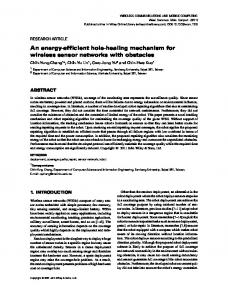
To provide an optimal benchmark for the simulation, the network routing problem presented in equation (3.7) was modeled as a Mixed Integer Linear Problem (MILP) in GAMS (GAMS, 2016) and solved by CPLEX 12 solver (IBM, n.d.). To solve the problem to optimality, we altered CPLEX options of relative termination tolerance to 0 (optcr=0.0) and the maximum time allocated in wall clock seconds from the default value of 1000 to 500000 seconds (reslim = 500000). We solved each network for all the flows provided in Table 5.1 and compared our proposed solution to the optimal solution. Flows origin and destination pairs were generated using a uniform random distribution function and flow rate was bounded between a random number between 50 to 200, i.e. , rf 2 [50, 200].
51
Table 5.1: Networks Used for Evaluation Network
Flows
Abilene Atlanta Polska Nobel-US Nobel-Germany New York
132 210 66 91 121 240
Nodes
Links
Avg Node Degree
Link Density
12 15 12 14 17 16
15 22 18 21 26 49
2.50 2.93 3.00 3.00 3.06 6.12
22.73 % 20.95 % 27.27 % 23.08 % 19.12 % 40.83 %
Abilene
Nobel-US
Polska
Nobel-Germany
Atlanta
New York
Figure 5.2: Network Topologies
Each link in the topology operates at a discrete rate. The discrete rates used in our evaluation were obtained from the specifications in the Intel Ethernet Controller X540 datasheet. The X540 Ethernet Controller supports three transmission rates 100 Mbps, 1 Gbps and 10 Gbps as shown in Table 4.1.
52
Table 5.2: Intel Ethernet Controller X540 Power Measurements Discrete Rates 100 Mbps 1 Gbps 10 Gbps
Power Consumption 3.2 W 4.27 W 7.7 W
We explore the quality of the solution provided by our solution and show that results obtained are close to the optimal solution provided by CPLEX. Similar to our constraint generation procedure, GAMS generates the appropriate equations for each constraint. It then, tries find in a combinational manner the set of variables that satisfy all constraints and minimize the objective value. Due to the nature of this combinational procedure, the solution provided is guaranteed optimal. We implemented the problems in Matlab 2015 version B (Mathworks, 2015). By interfacing Matlab and GAMS using the GAMS Data Exchange (GDX) framework, we were able to change input parameters to introduce a different flows and topologies that are read from the XML instance provided by SNDLib and converted to structures compatible with GAMS.
53
5.4.2
Different Networks Evaluation
5.4.2.1
Cost Evaluation
Optimal
Proposed
SP
Power Consumption (W)
250 200 150 100 50 0 - US
Nobel Germany
NewYork
74.59
91.53
114.95
114.57
107.11
76.47
92.90
118.40
118.30
159.26
101.28
130.17
156.25
259.27
Abilene
Atlanta
Polska
Optimal
82.28
105.28
Proposed
83.33
Shortest Path
110.36
Nobel
(a)
Error %
8 6 4 2 0
Average Error %
Abilene
Atlanta
Polska
Nobel -US
NobelGermany
NewYork
1.33%
1.76%
2.50%
1.51%
3.01%
3.27%
(b)
Figure 5.3: Network Total Power Consumption (a) and percentage error of the proposed solution results in relation to the optimal (b). (Awad, Rafique, & M’Hallah, 2017)
Shortest-path routing routes each flow individually on the least hop-based path, without considering the cost induced. Therefore, traditional shortest path routing is the least energy efficient routing choice as shown in Figure 5.3a. Our proposed solution was able to provide an energy efficient routing solution within 0 % to 3.27% difference from the 54
optimal routing solution. For the Abilene, Atlanta and New York networks we were able to achieve a solution that matched the optimal solution exactly. However, we noticed a 1 % difference for Nobel-US, a 3 % difference for Nobel-Germany and a 4 % difference for Polska. The error difference is is proportional to the network complexity, that is significantly impacted by the number of links in the network topology. These differences occur due to the nature of our proposed solution, where begins by initializing all flow paths to by routing them on their shortest-path. It iteratively tries to reroute flows which are causing excess in the network. The order of selection of these flows highly impacts the quality of the solution. Our proposed solution is capable of providing a high quality solution overall.
5.4.2.2
Energy Savings Evaluation
Optimal
Proposed
Power Savings Ratio%
50 40 30 20 10 0 - US
Nobel Germany
NewYork
26.15%
29.64%
26.32%
55.79%
24.22%
28.58%
24.12%
54.35%
Abilene
Atlanta
Polska
Optimal
25.44%
33.88%
Proposed
24.47%
32.72%
Nobel
Figure 5.4: Power saving compared to SP network power consumption. (Awad, Rafique, & M’Hallah, 2017)
We compute energy savings ratio for our proposed solution and CPLEX and compare them to traditional shortest path routing as shown in Figure 5.4. Results shown, reveal that the proposed solution brings significant energy savings compared to shortest path 55
routing, ranging between 24.22% up to 54.35%. It was observed that there is greater potential for power saving in highly connected networks like New York that has a link density of 40.88%, where 54.35% energy savings was achieved. On the other hand, lightly connected networks like Nobel-Germany, with a link density of 19.12%, achieved only 24.42% energy savings. Higher connected networks offer an abundance of alternative links for the algorithm to conduct necessary rerouting. The power saving of the Abilene, Polska, Noble-US and Atlanta networks with proportional link density, depends on the number of links in the network. The larger the number of links, the larger the power saving. The proposed solution increases network energy efficiency by combining flows paths together to decrease the total number of active links. On the contrary, shortest path handles each flow individually by routing it on the shortest path between origin and destination, thus enabling all required links on that path regardless of the total networking cost.
Computational Time Evaluation
Optimal
106
Proposed
25
105
20
104
15
103
10
102
5
101
0
100 Abilene
Atlanta
Polska
Nobel - US
Nobel Germany
NewYork
Optimal
78.85
19684.89
988.28
Proposed
4.32
11.49
4.61
7532.06
9587.72
76007.12
7.87
11.66
24.39
CPLEX (Seconds)
Proposed Solution (Seconds)
Computation Time of
30
Computation Time of
5.4.2.3
Figure 5.5: Computation time of the proposed solution and CPLEX. (Awad, Rafique, & M’Hallah, 2017)
56
Our proposed solution converged to the solution with an average of 10.72 seconds, compared to the optimal solution’s average of 5.27 hours. Results shown in Figure5.5 illustrate that higher network connectivity as shown in Table 5.1 is associated with higher computational time. A lightly connected network, Abilene with a 22.73% link density and 132 flows was solved in about 4 seconds, while optimal solution required about 79 seconds to converge. We observed that in networks with comparable complexities, the number of flows to be routed impacted the computational time significantly, i.e., Atlanta with 210 flows and consumed 3.62 seconds more than Nobel-Germany with equivalent network complexity. Furthermore, highly connected networks like New York with a link density of 40.83% and 240 flows are extremely computationally expensive requiring 21.11 hours to converge, while the proposed solution remarkably solves it in only 24.39 seconds. Computation time increases as the network complexity and the number of flows increases as a consequence of more alternative links and a larger room for combination among network flows.
57
5.4.2.4
Average Number of Hops Evaluation Optimal
Proposed
SP
Average Number of Hops
6 5 4 3 2 1 0 -US
NobelGermany
Atlanta
NewYork
4.32
5.58
6.24
4.82
4.55
3.12
2.80
2.98
3.15
3.27
2.23
2.42
2.16
2.17
2.78
2.49
1.69
Abilene
Polska
Optimal
4.12
Proposed Shortest Path
Nobel
Figure 5.6: Average number of hops in various network topologies. (Awad, Rafique, & M’Hallah, 2017)
Average number of hops is calculated by calculating the average number of nodes traversed by each flow on the path the origin to the destination. As shown in Figure 5.6 shortest path routing proves to be the lower bound to the average number of hops. Results demonstrate that despite the speed and accuracy of the proposed solution, network performance measured in the average number of hops has not been significantly affected. Furthermore, the proposed solution exceptionally outperformed the optimal solution. The average number of hops of the proposed solution was only 28% higher than the shortest path, while the optimal solution yielded a solution 116.11% higher than the lower bound. Our scheme favors a lower number of hops as a consequence of using Yen’s K-Shortest Path routing algorithm (Yen, 1971) that reroutes flows with the basis of shortest alternative first; see Algorithm 1 Line 9. Therefore, it starts with the shortest possible path and then iteratively tries to reroute them in the most cost effective way until a feasible solution is determined, simultaneously favoring network performance. On the contrary, optimal solution modeled in equation (3.7) does not account for minimizing the number of hops in 58
its objective function. Instead it favors combining flows in such a way that link bandwidth is served at the least possible discrete link rate, in most cases leading to a longer flow path.
5.4.2.5
Utilization Evaluation Optimal
80
Proposed Solution
Shortest Path
Utilization %
70 60 50 40 30 20 10 0 Abilene
Polska
Nobel - US
Nobel Germany
Atlanta
NewYork
Optimal
43.37
19.20
37.04
38.06
80.38
85.20
Proposed Solution
40.78
19.44
22.36
29.57
61.01
44.33
Shortest Path
25.40
9.65
10.60
16.88
30.44
10.97
Figure 5.7: Different Networks Average Link Utilization (Awad, Rafique, & M’Hallah, 2017)
Link utilization is an indicator representing the amount of total flow passing on each link in comparison to the link capacity of 10 Gbps. Figure 5.7 shows that optimal solution is able to achieve the highest link utilization, while shortest path routing achieves the least. Even though link utilization is not explicitly modeled in equation (3.7), the combinational nature of the CPLEX solver leads to the appropriate flows to be selected in such a way that the total flows installed on each link is closest to the discrete operating level, as shown in the previous section in most cases this leads to each flow being routed on a longer path. On the contrary, our VCG algorithm initially routes all flows on the shortest path and then iteratively selects flows on links with excess values to be rerouted, the selection of these flows is done in the best effort to maximize the total amount of flows passing through each 59
link. However, certain links remain with only a few flows passing through them, leaving them under utilized and affecting the network average. Despite this, the total number of links in the network are the same as the optimal solution leading to similar final routing cost, but they differ with the choice of links selected. Shortest path routing performs the worst in terms of link utilization, specially in highly connected networks like New York where it achieves 10.97 % link utilization because there are enough link for almost each flow to reserve a path on its own. The average link utilization for all networks was 50.54 % for the optimal solution, 36.25 % achieved by our solution and 17.3 % by the shortest path.
5.4.3
Variation of Number of K Alternative Paths 300 Abilene Polska
250
Nobel-US Nobel-Germany Atlanta New York
Cost (W)
200
150
100
50
2
4
6
8
10
12
14
Number of K Alternative Paths
Figure 5.8: Impact of Variation of K-Alternative Paths on the Cost (Awad, Rafique, & M’Hallah, 2017)
The K-Shortest Path algorithm generates multiple alternative paths starting with the shortest hop based alternative path. In this section we alternate K between K = 1 up to 60
K = 15 and run our proposed algorithm for all networks to evaluate the impact it has on the quality of the solution. Figure 5.8 demonstrates the exponential effect incrementing the number of alternative paths has on the solution. In the New York network, the solution starts with a 58 % error, the error drops radically as we reach K = 6 converging to 14 %. We notice that addition of K alternative paths starts to converge forming into a steady solution. Therefore, we conclude that K = 15 is a reasonable number of alternative paths to provide an accurate solution for all networks. It is important to note that the number of K-alternative paths should be limited, as it directly effects the computational complexity. Each flow has to be re-routed on all the alternative paths in each iteration of the algorithm, where the most cost feasible alternative is chosen.
5.4.4
Convergence
Our scheme is based on a constraint generation approach, that exhibits an iterative nature. Constraints are added by the VCG Algorithm and are sent to the LRC Algorithm to satisfy the violated constraints. Constraints are continually generated in each iteration and are appended to the pool of constraints until the algorithm converges to the optimal solution. The algorithm can only converge to the optimal solution when the pool of constraints is large enough to account for all flow violations in the network. The number of iterations required to reach to the optimal solution is the convergence speed. As shown in Figure 5.9, the Abilene network was solved with 132 flows and the network routing cost was computed at each iteration. The algorithm converged to optimality, with a routing cost of 84.7 W in 34 iterations. Due to the fair complexity of the algorithm, these iterations were computed in just under 2.8 seconds running on our machine as compared to CPLEX’s optimal solution which required 1.5 hours to converge. The proposed solution was able to get within 18 % error from the optimal solution in just 13 iterations, while it later carried out appropriate flow rerouting to reach optimal feasibility, i.e., same as the CPLEX solution.
61
********************** Optimal Solution ************************* 80 70
Cost (W)
60 50 40 30 20 10
0
5
10
15
20
25
30
Number of Iterations
Figure 5.9: Algorithm Convergence (Awad, Rafique, & M’Hallah, 2017)
5.4.5
Single-Flow Routing Problem
In the previous sub-sections we focused on solving networks with the complete set of network flows concurrently. Solving all flows concurrently is not always network feasible, since it requires prior information about all network flows. However, in active networks flow requests are generated continuously. These requests have to be handled instantly as they arrive and the appropriate flow path has to be assigned. Appending the solution to accommodate for a additional flow is referred to as single flow routing problem. The proposed solution is capable of solving single flow routing problems by generating the necessary violated constraints and appending the pool of constraints that returns an updated solution that satisfies the additional flow request.
62
84
Cost (W)
82
80 Optimal Proposed Solution 78
76
74 60
70
80
90
100
110
120
130
Number of Iterations
Figure 5.10: Single-Flow Routing Cost (Awad, Rafique, & M’Hallah, 2017)
We routed 50% (66 flows) of the Abilene network and started iteratively introducing single flow requests to the network until all 132 were solved. For each iteration the impact on network routing cost and the additional time consumed by each flow was evaluated. Figure 5.10 shows that our scheme can achieve routing costs similar to the optimal solution provided by CPLEX. Our scheme can guarantee optimality without re-solving the entire problem. For some flows, e.g., 80 to 99, the existing link rates were sufficient to accommodate the additional 9 flows, hence the routing cost was not affected. However, when the 100th flow was added, the routing cost has increased due to an activation of an additional link to accommodate for the new flow.
63
Proposed Solution
3.5
7500
3.0
5000
2.5
2500
2.0
60
70
80
90
100
110
120
130
Optimal Solution Time (s)
Proposed Solution Time (s)
Optimal
0
Number of Iterations
Figure 5.11: Single-Flow Convergence Time (Awad, Rafique, & M’Hallah, 2017)
Figure 5.11 presents the computational time of each additional flow for both the proposed solution and the optimal solution. Due to the large difference in the computational times, results were plotted on two different y-axis. The left axis presents the computational time of the proposed solution, while the right axis presents the computational time of the optimal solution. It can be deduced from the figure that on average, the proposed solution consumed 22 milliseconds for each additional flow request, while CPLEX consumed an average of 86.26 seconds. In addition, the total time consumed by the proposed solution to route the additional 66 flows was 1.43 seconds, while CPLEX required a total of 1.58 hours to solve the same number of flows.
Time consumed in the scheme’s convergence is entirely dependent on the number of iterations produced. If there exists a set of links on its flow path with enough spare capacity to satisfy the additional flow, then no constraints are added and the solution, thereby converging with no further iterations. However, if the additional flow cannot be routed due to the lack of spare capacity, causing an excess. To minimize the network excess caused by the additional flow existing flows have to be re-routed on alternative 64
paths in the most energy efficient manner by the VCG algorithm in order to eliminate excess in the network. After VCG termination, a violation still exists, violated constraints are generated and LRC has to iteratively carry out capacity changes until feasibility is achieved.
5.4.6
Multi-Flow Routing Problem
To mimic real network scenarios, it is impractical to expect a single flow requests arriving at a given time instance. Instead, we should expect multiple flow requests to arrive simultaneously, this is referred to as the multi-flow routing problem. To demonstrate our scheme’s capability to solve such problems we ran the same setup presented for single flow routing, but rather than introducing a single flow per iteration, we introduced 10 flows per iteration until we have solved for all network flows.
84
Cost (W)
82
Optimal Proposed Solution
80
78
76
74 70
80
90
100
110
120
130
Number of Additional Flows
Figure 5.12: Multi-Flow Routing Cost (Awad, Rafique, & M’Hallah, 2017)
Starting at 72 demands we introduced 10 multi-session flows per run and plotted the 65
cost change in Figure 5.12. Costs presented by our solution exhibit a trend similar to the optimal solution’s cost, justifying that the appended solution is in fact similar to the optimal solution in terms of energy efficiency. The cost increases when current active links are not enough to satisfy flows as 10 simultaneous flow requests enter the network and additional links need to be turned on. We can observe that starting from 72 flows, the addition of 10 flows each time lead to a significant increase in cost, due to existing links did not have spare capacity enough to satisfy the number of incoming flow requests. This in-turn cased a violation in VCG and induced an increased cost due to the activation of additional links by the LRC. Increasing the number of flows from 82 to 92 did not require an increase in the number of iterations since active links were able to satisfy them.
Proposed Solution 750
2.5
500
2.25
250
2.0
Optimal Solution Time (s)
Proposed Solution Time (s)
Optimal 2.75
0 60
70
80
90
100
110
120
130
Number of Additional Flows
Figure 5.13: Multi-Flow Convergence Time (Awad, Rafique, & M’Hallah, 2017)
Figure 5.13 shows the time required to solve for the additional multiple flows entering the network at an instance of time. The time consumed by our proposed solution is shown on the left vertical axis, while the time consumed by the optimal solution is shown on the right vertical axis. Our solution takes on average 58 ms to solve for every multi-flow problem consuming a total additional time of 0.35 seconds to solve for all network flows 66
starting from a solution of 72 flows. The optimal solution on the other hand, consumes around 138 seconds to solve each multi-session problem and a total of 825 seconds to solve all network flows, since it has to resolve the entire problem. This justifies that our algorithm is able to provide high quality solutions with realistic and acceptable delay times. The proposed solution was able to solve the routing problem rapidly due to the smart constraint generation process, where it required only an addition of 7 algorithm iterations to route all the additional network flows.
67
CHAPTER 6
CONCLUSION
In this thesis, we introduced practical network constraints and evaluated their significance on the performance of energy-aware routing schemes in SDN networks. We modeled the routing problem as a MIP problem and considered discrete link rates and flow rules limitation in the problem formulation. We demonstrated how to model the mathematical equations in GAMS and integrated the model with MATLAB through the GDX framework to alternate the input parameters. We then presented simulation results and compared them to traditional routing to confirm that discreteness of link rates and limitation of flow rules space has major impact not only on the energy efficiency of SDNs but also on network performance.
Computing optimal routing solution using commercial solves like CPLEX that was shown to be computationally expensive. We presented an implementation of a fast heuristic algorithm that solves the routing problem in network feasible time. The algorithm is based on the benders mathematical decomposition method and the problem is modeled as a MIP problem (Awad, Rafique, & M’Hallah, 2017). The proposed solution was based on two algorithms namely, VCG and LRC. The proposed solution is capable of providing a near optimal solution when compared to CPLEX, providing an error rate less than 3.27%. Performance of the proposed solution was compared with CPLEX and shortest path routing and was evaluated for six different networks with various network characteristics and complexities. The benders-based solution proved to be exceptionally advantageous over shortest path routing and attained 54.35% power savings. Moreover, it was designed to work independently on simple hardware with minimal computational power, without the need for external commercial solvers. Details on the implementation have been provided 68
in the appendix.
The solution proposed in this work was designed to run on the most basic networking devices with single processor computational power. Future work includes the introduction of parallelization techniques to the enhance the performance of the benders decomposition based heuristic. The benders solution is very amenable to parallelization, due to the nature of the problem breakdown, where each sub-problem can be solved separately. We plan to implement our solution in the Network Simulator-3 (NS-3) environment (Riley & Henderson, 2010). NS-3 simulation environment facilitates SDN simulations since it offers built in support for OpenFlow enabled switches. It will allow us to not only test our solution under real network topologies, but also to evaluate different metrics such as packet routing ratio, throughput, end-to-end delay and bit error rate.
69
REFERENCES
Awad, M. K., El-Shafei, M., Dimitriou, T., Rafique, Y., Baidas, M., & Alhusaini, A. (2017). Power-efficient routing for sdn with discrete link rates and size-limited flow tables: A tree-based particle swarm optimization approach. International Journal of Network Management, e1972–n/a. Retrieved from http://dx.doi.org/10.1002/ nem.1972 (e1972 nem.1972) doi: 10.1002/nem.1972 Awad, M. K., Neama, G., & Rafique, Y. (2015, Nov). The impact of practical network constraints on the performance of energy-aware routing schemes. In 2015 IEEE international conference on service operations and logistics, and informatics (soli) (p. 7781). doi: 10.1109/SOLI.2015.7367595 Awad, M. K., Rafique, Y., Alhadlaq, S., Hassoun, D., Alabdulhadi, A., & Thani, S. (2016). A greedy power-aware routing algorithm for software-defined networks. In Signal processing and information technology (isspit), 2016 ieee international symposium on (pp. 268–273). Awad, M. K., Rafique, Y., & M’Hallah, R. A. (2017). Energy-aware routing for software-defined networks with discrete link rates: A benders decomposition-based heuristic approach. Sustainable Computing: Informatics and Systems, 13, 31 - 41. Retrieved from http://www.sciencedirect.com/science/article/pii/ S2210537916301251 doi: http://dx.doi.org/10.1016/j.suscom.2016.11.003 Banerjee, S., & Kannan, K. (2014). Tag-in-tag: Efficient flow table management in sdn switches. In Network and service management (cnsm), 2014 10th international conference on (pp. 109–117). Caesar, M., Caldwell, D., Feamster, N., Rexford, J., Shaikh, A., & van der Merwe, J. (2005). Design and implementation of a routing control platform. In Proceedings of the 2nd conference on symposium on networked systems design & implementation-volume 2 (pp. 15–28). Carrega, A., Singh, S., Bruschi, R., & Bolla, R. (2012). Traffic merging for energyefficient datacenter networks. In Performance evaluation of computer and telecommunication systems (spects), 2012 international symposium on (pp. 1–5). Casado, M., Garfinkel, T., Akella, A., Freedman, M. J., Boneh, D., McKeown, N., & Shenker, S. (2006). Sane: A protection architecture for enterprise networks. In Usenix security. Committee, O., et al. (2012). Software-defined networking: The new norm for networks. Open Networking Foundation. Controller, I. E. (2016). X540 datasheet rev. 3.0. Intel Corporation, January. 70
CPLEX, I. I. (n.d.). 12.6, 2013. Ferris, M. C., Jain, R., & Dirkse, S. (2011). GDXMRW: Interfacing GAMS and MATLAB. Online: http://www. gams. com/dd/docs/tools/gdxmrw. pdf . Gabrel, V., Knippel, A., & Minoux, M. (1999). Exact solution of multicommodity network optimization problems with general step cost functions. In (Vol. 25, pp. 15–23). Elsevier. Gabrel, V., Knippel, A., & Minoux, M. (2003). A comparison of heuristics for the discrete cost multicommodity network optimization problem. Journal of Heuristics, 9(5), 429–445. GAMS. (2016, 24.8). Retrieved from https://www.gams.com Giroire, F., Moulierac, J., & Phan, T. K. (2014). Optimizing rule placement in softwaredefined networks for energy-aware routing. In Global communications conference (globecom), 2014 IEEE (pp. 2523–2529). Glanz, J., & Sakuma, P. (2011, September). Google details, and defends, its use of electricity (Vol. 8). Retrieved from http://www.nytimes.com/2011/ 09/09/technology/google-details-and-defends-its-use-of -electricity.html Greenberg, A., Hjalmtysson, G., Maltz, D. A., Myers, A., Rexford, J., Xie, G., . . . Zhang, H. (2005). A clean slate 4d approach to network control and management. ACM SIGCOMM Computer Communication Review, 35(5), 41–54. Gude, N., Koponen, T., Pettit, J., Pfaff, B., Casado, M., McKeown, N., & Shenker, S. (2008). Nox: towards an operating system for networks. ACM SIGCOMM Computer Communication Review, 38(3), 105–110. IBM. (n.d.). 12.6. Retrieved 2013, from https://www-01.ibm.com/software/ commerce/optimization/cplex-optimizer/ Index, C. V. N. (2016). Cisco visual networking index: Forecast and methodology 20152020. White paper, CISCO (June 2016). Instance, A. N. P. (n.d.). Sndlib–library of test instances for survivable fixed telecommunication network design. Retrieved from http://sndlib.zib.de Mathworks. (2015, B). Matlab. Retrieved from http://www.mathworks.com/ products/matlab/ MathWorks, I. (2002). Curve fitting toolbox: for use with matlab®: user’s guide. MathWorks. Mrad, M., & Haouari, M. (2008). Optimal solution of the discrete cost multicommodity network design problem. Applied Mathematics and Computation, 204(2), 745–753.
71
Nunes, B. A. A., Mendonca, M., Nguyen, X.-N., Obraczka, K., & Turletti, T. (2014). A survey of software-defined networking: Past, present, and future of programmable networks. IEEE Communications Surveys & Tutorials, 16(3), 1617–1634. Rafique, Y., Awad, M. K., & Neama, G. (2017, May 8-11). A benchmark implementation for evaluating the performance of power-aware routing algorithms in practical software-defined networks. The Fourth International Conference on Software Defined Systems (SDS). Riley, G. F., & Henderson, T. R. (2010). The ns-3 network simulator. Modeling and tools for network simulation, 15–34. Rosenthal, R. E. (2008). GAMS: a user’s guide. 2008. Washington, DC, USA: GAMS Development Corporation. Specification, O. S. (2011). Version 1.2 (wire protocol 0x03). Open Network Foundation. Stoer, M., & Dahl, G. (1994). A polyhedral approach to multicommodity survivable network design. Numerische Mathematik, 68(1), 149–167. Wanderer, J. (2013). Case study: The google sdn wan. Computing. co. uk, 11. Wang, L., Anta, A. F., Zhang, F., Hou, C., & Liu, Z. (2013). Routing for energy minimization with discrete cost functions. arXiv preprint arXiv:1302.0234. Yen, J. Y. (1971). Finding the k shortest loopless paths in a network. Management Science, 17(11), 712–716.
72
APPENDIX
Main Program
Initialization clc; clear;
% XML network instances provided from
Survivable fixed
telecommunication Network Design (SNDLib) % Available Online: http://sndlib.zib.de %Choice of networks to read from XML file: abilene / atlanta / polska / nobel-us / nobel-germany / newyork NetworkName =’abilene’;
%Network Instance file path [ XMLStruct ] = xml2struct( strcat(’Instances/’, NetworkName, ’.xml’) ) ;
%Reads Flows from the XML Struct & constructs a stuct of Flows FlowsXMLStruct = XMLStruct.network.demands.demand; TotalFlowsRead= size(FlowsXMLStruct,2);
NoOfIterations = 500;
% Maximum Number of iterrations for
algorithm LinkCap
= 10000;
% Maximum Link Capacity
% Discrete Link Rates Rates = [0, 100, 1000, 10000];
NoOfRates = size(Rates,2);
73
% Link Costs Cost = [0, 3.2, 4.27, 7.7];
%Read Nodes from XML NodesXMLStruct = XMLStruct.network.networkStructure.nodes.node; NoOfNodes = size(NodesXMLStruct,2); NodeNames = cell(1,NoOfNodes); for N=1:NoOfNodes NodeNames{N} = NodesXMLStruct{N}.Attributes.id; end clearvars
NodesXMLStruct;
% To Read links from XML File TopologyXMLStruct = XMLStruct.network.networkStructure.links.link;
% Build Topology [Topology, LinkMatrix, NoOfLinks, LinkNames ] = BuildTopology( NoOfNodes, TopologyXMLStruct, NodeNames); NoOfKPaths = NoOfLinks;
%Converts Topology to 1’s and inf for compatability with dijkstra G(NoOfNodes,NoOfNodes) = zeros; G(Topology == 1)=1; G(Topology == 0)=inf;
NoOfFlows = TotalFlowsRead;
%Name of Each Flow FlowNames = cell(1,NoOfFlows);
%Size of Each Flow FlowSizes(NoOfFlows) = zeros;
%ShortestPath of each flow ShortestPath = cell(1,NoOfFlows);
74
%K-ShortestPaths of each flow KShortestPaths = cell(1,NoOfFlows);
% Number of Links a flow passes through on its path from source to destination PathLength(NoOfFlows) = zeros;
% Path of each Flow FlowPath = cell(1,NoOfFlows);
%Constrcts the FlowConserve tables FlowConserve(NoOfNodes, NoOfFlows) = zeros;
for F= 1:NoOfFlows
%Different seed based on Flow Index rng(F,’twister’); s = rng;
% Random Flow Size Generation for Each Flow distributed uniformly between [50-200] FlowSizes(F) =
round((200-50).*rand(1,1) + 50);
% Assign Flow Names {Flow1, Flow2, ... , FlowF} FlowNames{F} = strcat(’Flow’,int2str(F));
% Random Source / Destination Generation for each Flow Source = int64(1 + (NoOfNodes-1).*rand(1,1)); Target = int64(1 + (NoOfNodes-1).*rand(1,1)); count = 0; while(Source == Target) rng(F*(count+1),’twister’); s = rng; Source = int64(1 + (NoOfNodes-1).*rand(1,1)); rng(F*(count+2),’twister’); s = rng; Target = int64(1 + (NoOfNodes-1).*rand(1,1));
75
count = count+1; end SourceIndex = Source; TargetIndex = Target; FlowConserve(SourceIndex,F) = FlowSizes(F); FlowConserve(TargetIndex,F) = -FlowSizes(F); [ShortestPath{F}, PathLength(F)] = dijkstra(G, SourceIndex, TargetIndex); [KShortestPaths{F}, ˜] = kShortestPath(G, SourceIndex, TargetIndex, NoOfKPaths); FlowPath{F} = ShortestPath{F}; end
% Set of Metric Inequalities for each iteration MetricInequalities(NoOfIterations) = zeros;
% Flow on Links LinkRate(NoOfLinks) = zeros;
% Binary Link Cost Indicating whether Link in G is ON / OFF LinkCostPerIter(NoOfLinks, NoOfIterations) = zeros; LinkCost(NoOfLinks) = zeros;
% Summation of all Flow Sizes passing on a certain link LinkBandwidth(NoOfLinks) = zeros;
%Binary Indicating whether Flow is passing on a certain link FlowOnLink(NoOfLinks, NoOfFlows)=zeros;
% Amount of Flow Required on each Link to route Flows Excess(NoOfLinks) = zeros;
tic; %Start Timer
Algorithm Starts for iter= 1:NoOfIterations
76
fprintf(’\n ************************ Iteration # %d ************************** \n’, iter); [ FlowPath ] = VCG( LinkRate, NoOfLinks, NoOfFlows, FlowSizes, LinkMatrix, NoOfKPaths, FlowPath, KShortestPaths );
LinkBandwidth(:) = 0;
FlowOnLink(:,:) = 0; for F=1:NoOfFlows for Path = 1:size(FlowPath{F},2)-1 Source = FlowPath{F}(Path); Target = FlowPath{F}(Path+1); LinkIndex = find(LinkMatrix(Source,Target,:)); FlowOnLink(LinkIndex, F) = 1; LinkBandwidth(LinkIndex) = LinkBandwidth(LinkIndex)+ FlowSizes(F); end end LinkBandwidth = round((LinkBandwidth*1000))/1000; Excess(:) = 0; %Based on the sum of Flows passing through each link compute excess required for LinkIndex = 1:NoOfLinks Excess(LinkIndex) =
(LinkBandwidth(LinkIndex) - LinkRate(
LinkIndex)); end Excess = round((Excess*1000))/1000; Excess(Excess < 0)=0;
%Recompute NetExcess based on new Excess after re-routing NetExcess =
(sum(Excess(:)));
NetExcess = round((NetExcess*1000))/1000; PathLength(:) = 0;
77
%Calculate # of Hops for F=1:NoOfFlows for Path = 1:size(FlowPath{F},2)-1 Source = FlowPath{F}(Path); Target = FlowPath{F}(Path+1); LinkIndex = find(LinkMatrix(Source,Target,:)); if (Excess(LinkIndex) > 0) PathLength(F) = PathLength(F) +1; end end end
LinkCost(:) = 0; for LinkIndex = 1:NoOfLinks if (Excess(LinkIndex) > 0) LinkCost(LinkIndex) = 1; end end
%Record variables in each iteration LinkCostPerIter(:,iter) = LinkCost;
%If no violated constraints found, terminate. if(NetExcess ==0) break; end
MetricInequalities(iter) = dot(PathLength,FlowSizes);
%Call LRC Algorithm [LinkRate] = LRC(iter, LinkRate, MetricInequalities, LinkCostPerIter, NoOfLinks, Rates, Cost, Excess);
IterCost = 0;
for Path = 1:NoOfLinks
78
if (LinkRate(Path) > Rates(1) && LinkRate(Path) Rates(2) && LinkRate(Path) Rates(3) && LinkRate(Path) Rates(1) && OnLinks(Path) Rates(2) && OnLinks(Path) Rates(3) && OnLinks(Path)