Saad, A., et al.: An Improved Computational Method for Non-Isothermal … THERMAL SCIENCE, Year 2011, Vol. 15, Suppl. 2, pp. S275-S289
S275
AN IMPROVED COMPUTATIONAL METHOD FOR NON-ISOTHERMAL RESIN TRANSFER MOULDING SIMULATION by
Aouatif SAAD a*, Adil ECHCHELH a, Mohammed HATTABI b, and Mohammed El GANAOUI c a
Laboratory of Electrical Engineering and Energetic Systems, Faculty of Sciences, Ibn Tofail University, Kenitra, Morocco b Applied Research Team on Polymers, Department of Mechanical Engineering, ENSEM, Hassan II University, Oasis, Casablanca, Morocco c Université de Lorraine, LERMAB-Longwy, IUT Henri Poincaré, Nancy, France Original scientific paper UDC: 621.744:517.96 DOI: 10.2298/TSCI100928016S
The optimization in the simulation time of non-isothermal filling process without losing effectiveness remains a challenge in the resin transfer moulding process simulation. We are interested in this work on developing an improved computational approach based on finite element method coupled with control volume approach. Simulations can predict the position of the front of resin flow, pressure and temperature distribution at each time step. Our optimisation approach is first based on the modification of conventional control volume/finite element method, then on the adaptation of the iterative algorithm of conjugate gradient to compressed sparse row storage scheme. The approach has been validated by comparison with available results. The proposed method yielded smoother flow fronts and reduced the error in the pressure and temperature pattern that plagued the conventional fixed grid methods. The solution accuracy was considerably higher than that of the conventional method since we could proceed in the mesh refinement without a significant increase in the computation time. Various thermal engineering situations can be simulated by using the developed code. Key words: resin transfer moulding, control volume/finite element method, conjugate gradient, sparse matrix
Introduction
In today’s highly competitive global economy, the need for materials with the right properties to meet the demands of design, environment, durability, and economics is growing. Composite materials, with their high strength and stiffness-to-weight ratios, have many advantages and are a desirable engineering material. Thousands of products are moulded each year utilizing reinforced composites: aerospace [1], automotive parts [2], sports, electric and recreational equipment, boats, and business machines to name a few. *nCorresponding author; e-mail:
[email protected]
S276
Saad, A., et al.: An Improved Computational Method for Non-Isothermal … THERMAL SCIENCE, Year 2011, Vol. 15, Suppl. 2, pp. S275-S289
Among a variety of composite moulding process, resin transfer moulding (RTM) offer the maximum design versatility and excellent cost/performance characteristics. In RTM process; a special formulated thermosetting resin is injected into a closed mould containing the dry reinforcement material that has been shaped into a preformed piece. After the mould is completely filled, the resin cures due to higher temperature of the mould. The mould filling process is a very important and complex step in the RTM, governing the performance of the final product and tool design. It is affected by several parameters comprising of mould geometry, inlet gate(s) location, injection pressure or flow rate, resin rheology, permeability and thermal conductivity of fibrous media, and temperatures of mould wall and inlet resin. Heat transfer from the mould wall decreases the resin viscosity and reduces the mould filling time, but the temperature rise activates the curing reaction, leading to significant temperature gradient [3], which leads to residual stresses in the part. Optimization of all earlier-mentioned parameters by experimental works is a costly and time-consuming task. Alternatively, thermal engineering has become a cost effective tool, it demonstrates its applicability and its ability to understand thermo mechanical phenomena involved during the various stages of RTM process, whose inclusion is of definite need for a better prediction of optimum parameters that can design the composite parts with high performance and low cost. Heat transfer continues to be a major field of interest to engineering and scientific researchers, as well as designers, developers, and manufacturers. A variety of numerical studies has been interested on the simulation of heat transfer and resin curing during the RTM process, Choi et al. [4] have developed a methodology to manage the heat generated by the cure reaction that minimizes the temperature gradients before the resin solidify. Guo et al. [5] have studied the filling and curing of tick composite parts, Lam et al. [6] have interested on the determination of an improved kinetic model suitable to tick composite part. Tuncol et al. [7] have developed a mathematical model based on 1-D flow and 2-D unsteady energy conservation to investigate the heat transfer between resin and mould walls. The RTM filling process is considered as a free boundary problem that have been simulated over the past decade [8-12]. This problem has been studied by two different procedures; the first one is a moving grid scheme; it often gives accurate representation of flow front position. But, since the calculation domain should be remeshed at each time step, it is computationally very time consuming and very difficult for the mould with inserts or multiple injection gates. Trochu et al. [13], and Hattabi et al. [14] have proposed numerical simulations based on boundary-fitted co-ordinates finite difference method. Yoo et al. [15] developed the boundary element method for mould filling process. A numerical simulation based on finite element method was proposed by Chan [16] using quadrilateral elements to study isothermal and non-isothermal filling but the applications were limited to rectangular moulds. The second approach is fixed grid mesh that is based on a control volume (CV) finite element (FE) method. This later has become the most versatile and computationally efficient way to solve the filling process. In this method one does not need to regenerate the mesh, since a fixed grid scheme is used. Fixed grid simulation is very useful for processes of material growth involving solid/liquid phase change as it is prouved by El Ganaoui et al. [17]. Shojaei et al. [18] simulated mould filling process using FE/CV formulations. They employed Galerkin finite elements to solve the pressure in the solution domain and used a CV approach to find the flow front location at each time step. The RTM process has been the subject of many experimental and numerical studies. But the major barrier encountered here is the simulation time, since a mould with a few thousands of nodes requires many hours of calculation. We are therefore interested in our study to
Saad, A., et al.: An Improved Computational Method for Non-Isothermal … THERMAL SCIENCE, Year 2011, Vol. 15, Suppl. 2, pp. S275-S289
S277
optimize the time of calculation and occupation memory of the numerical simulation method. This is done by the modification of the conventional FE method and secondly by the adaptation of the classical conjugate gradient algorithm to the compressed sparse row (CSR) storage scheme. The improved algorithm is then used to predict heat and mass transfers within the RTM process. Basic considerations Resin flow model
During mold filling, resin flows through a fiber bed. The filling process can be studied based on a microscopic or a macroscopic scale. Since the microscopic approach deals with the complicated local flow field between the fiber bundles, the macroscopic approach has become a common approach for simulation of the RTM process. In macroscopic approach, the filling process can be regarded, as liquid flowing through porous media, where we assume that the flow is fully saturated, such an assumption allows one the use of the quasisteady-state approximation for the flow of resin. Thus, the continuity equation for an isothermal incompressible fluid flow inside a fiber preform is expressed as:
V 0
(1)
To describe the flow within the mold, Darcy’s law has used :
K
V
P
(2)
Substituting Darcy’s law eq. (2) into continuity eq. (1) results in:
K where V is the volume-averaged Darcy’s velocity, K – the permeability tensor of the medium, m – the viscosity, and P – the pore-averaged resin pressure. In order to compute the mathematical model, the governing equation must be solved in conjunction with an appropriate set of boundary conditions (fig. 1) defined as:
P Pinj
at inlet gate
P Pfront at the flow front and P 0 at the mould wall n
P
0
(3)
Figure 1. A shematic representation of the mould
P 0 for all nodes P 0 for all nodes where 0 0 f 1 for all nodes
f
1
where f is a scalar parameter, called nodal fill fraction, showing the status of each control volume, is used to represent the filling status.
Saad, A., et al.: An Improved Computational Method for Non-Isothermal … THERMAL SCIENCE, Year 2011, Vol. 15, Suppl. 2, pp. S275-S289
S278
At the inlet, the resin is injected at a constant pressure Pinj, while in the front, the pressure is set to ambient pressure, at the mold wall a condition of no slip velocity is assumed. In the CV principle, the pressure is set to zero in empty and partially filled region, and it is different to zero in fully region. The fill factor comprises between 0 and 1 in all nodes of the mould cavity showing the status of the filling. Heat transfer model
As the resin fills the mould, heat transfer takes place between the resins, fiber perform, and mould walls. Heat may be generated by the resin curing which is an exothermic process. As a result, temperature variations are created throughout the mould cavity. These temperature variations influence the flow pattern by changing the viscosity which is a strong function of temperature. In analyzing the heat transfer, it is assumed that the resin and fiber reach local thermodynamic equilibrium as soon as the fiber is impregnated. This is justified because the heat transfer coefficient (eq. 4) between the resin and fiber is fairly large compared to the thickness of the fibers:
q (4) A T where q is the heat flow in input or lost heat flow, A – the heat transfer surface area, and DT – the difference in temperature between the fiber surface and surrounding resin area. Based on those assumptions, the heat transfer equation was: h
Cp
T t
r Cpr (V
T)
(
T)
HG
(5)
where l is the effective thermal conductivity, r – the density, Cp and Cpr are the heat capacity of the composite and resin, respectively, DH is the reaction heat, G – the reaction rate, and f – the porosity of the medium. In our work, one consider the case studied by Yu et al. [19] of a resin with constant viscosity and no source heat is observed, the eq. (5) becomes:
( where the effective thermal conductivity
T) 0
(6)
may be expressed by the rule of mixture [13]: r f r wf
f wr
f
wr
(8)
1 f
wf
(7)
r
1 wr
Indices f and r denotes fiber and resin, respectively.
(9)
Saad, A., et al.: An Improved Computational Method for Non-Isothermal … THERMAL SCIENCE, Year 2011, Vol. 15, Suppl. 2, pp. S275-S289
S279
To solve the eq. (6), boundary conditions must be specified at the injection ports, the mould walls, and the flow front. The possible boundary conditions could be:
T Tinj
at the inlet gate
T Tm at the flow front T 0 or T Tm at the mould wall n These conditions indicate that the temperature at the inlet is the incoming resin temperature, and at the flow front the fiber are initially considered at the mould temperature, at the mould wall the temperature is either fixed at the mould the temperature or a condition of no temperature flux is assumed. Numerical procedure
In this work, the FE/CV method was selected to solve the resin flow problem, because this fixed mesh method eliminates the need for remeshing the resin-filled domain for each time step, thus it has become the most versatile and computationally efficient way to simulate mold filling. Furthermore, the CV approach has certain attractive features: the formulation observes the conservation of mass and facilitates the translations from flux vectors into scalar flow quantities. The coupling of the CV concept with the FE method renders it ideal for simulating the filling process of complex parts including inserts. It is a combination of two very powerful techniques, blending accuracy of front tracking with the capability for modelling complex geometries. The CV-FEM numerical method combines a finite volume method to calculate the mass balance of the fluid phases while the fluid pressure field is computed implicitly using the FE method. Galerkin finite element formulation
The FE method is used to approximate the fluid pressure and temperature field at the FE nodes at each time step. The pressure is calculated by using the Galerkin procedure (3). Nodal pressure is evaluated by elementary matrices, and can be applied to all elements within the solution domain by applying an appropriate assembly procedure yielding a set of linear algebraic equations. By the same way the energy equation is treated and both leads to a matricial problem. Using calculated pressure, the velocities are then calculated at the “centroid” of each element (eq. 2). After the velocity of the resin computation, the CV technique is used to track the flow front position. Computational details
In the CV-FE approach, the mould cavity is first discretized into finite elements. By subdividing the elements into smaller sub-volumes, a CV is constructed around each node.
S280
Saad, A., et al.: An Improved Computational Method for Non-Isothermal … THERMAL SCIENCE, Year 2011, Vol. 15, Suppl. 2, pp. S275-S289
The concept of fill factor is introduced to monitor the fluid part in each CV. It is defined as a ratio of the volume of the fluid in the CV to the total volume. The fill factor varies between 0 and 1 (0 represents empty volumes and 1 filled ones, fig. 2). The numerical flow front is constructed of the nodes that have partially filled CV. At each time step, fill factors are calculated based on the resin velocity and flow in each nodal CV. If the resin does not gel, the flow front is thus updated until all the Figure 2. Model of filling of CV at the flow front control volumes are full. After the mould is disretized, the next step consists of the calculation of pressure and the velocity field for further determination of the flow front. In order to achieve computational economy, we will divide our optimisation approach into two parts, one first acted on the stiffness matrix derived from a FE formulation for the pressure and temperature field and then on the numerical algorithm of resolution. Optimization of stiffness matrix construction
In the conventional CV/FE approach [18], the stiffness matrix has the dimension of n n during all stage of filling where n is the number of node in the cavity. All components of the empty and partially filled CV are zero. Therefore, the stiffness matrix has several zero rows at the early stage of filling process. During filling algorithm, for a CV that the fill fraction reaches to the value 1, a single row should be added to the matrix corresponding to the node number. Hence, this led to an extensive use of memory and the execution time. For these reasons we are motivated to remedy to this by using the concept of dynamic matrix. This matrix wills no more to be statistical during the filling. Indeed, it has its dimension from the number of nodes that surrounding nodes of filled CV; so pressure and temperature are calculated in these nodes, while the pressure and temperature in the other nodes of the mould were automatically set to known boundary conditions. With these values of pressure the flow rate is calculated for neighbouring nodes, the fill factors are updated to select the filled CV. Once the node corresponding of filled CV is identified, the stiffness matrices must be updated to take in consideration new nodes that surround the filled CV, here one did not need to consider the entire elements in the assembling of the new stiffness matrices, only new elements had to be assembled and added to the old stiffness matrices. In the next iteration, the new matrices are now considered to calculate pressure and temperature distribution, the same steps are repeated as the first iteration and so one until the mould is completely filled. Resolution scheme
After the assembling of the stiffness matrices and imposing the boundary conditions, the system of equations is solved for unknown nodal temperature and pressure using an appropriate solver. Execution time, data representation, and numerical stability are the three such concerns of great interest that we tried to be assumed in our simulation.
Saad, A., et al.: An Improved Computational Method for Non-Isothermal … THERMAL SCIENCE, Year 2011, Vol. 15, Suppl. 2, pp. S275-S289
S281
Since the matrices are largely sparse and symmetric definite-positives, we have implemented an algorithm that take in account these proprieties, so our resolution scheme can be subdivided in two steps, the first concerns the storage of the matrix in a compressed format where only non-zero values are stored, where we are interested by the CSR storage format for the reason of its efficiency for all existing types of sparse matrices. The occupation memory is thus calculated by [20]:
nc 2nz n 1
(10)
where nc is the occupation memory, nz – the number of non-zero elements, and n – the matrix dimension. In the second step, we have adapted the classical iterative conjugate-gradient algorithm to the CSR storage format. We argued this choice of the iterative conjugate gradient solver by its fast convergence [21] by comparison with other direct and iterative solver and else more to its convenience to sparse and symmetric definite positive matrix. Results and discussion Validation of numerical results
The simulation results of the developed computer code, is compared with analytical solutions of some simple geometries for which the exact solution is known. In the simulation of the RTM filling process, the inlet condition can be either a constant volumetric flow rate or a constant injection pressure for the resin. Here constant pressure is taken as the inlet boundary condition. The details of physical properties of the fiber mats and resin are listed in tab. 1. The validation of our simulation code is carried out by two test cases. –
Table 1. Physical properties of fiber and processing conditions used in numerical study RTM parameters
Value
Pinj
4 ×10⁵ Pa
Kxx = Kyy
10–9 m2
m
0.4 Pa·s
f
0.5
kf
0.0335 W/mK
kr
0.168 W/mK
Cpf
670 J/kgK
Cpr
1680 J/kgK
Inline injection
The cavity used in this example is a rectangular mould with the dimensions 10 mm 2000 mm, the resin is injected at one surface of the rectangular mould and air is removed from the other surface resulting in 1-D flow. The analytical solutions for the rectilinear flow given by Cai [22] leads to a mould filling time of tf = fmL2/2KP0, a pressure field P(x) = P0 [1 – – x/xf(t)], and the flow front position is given by xf = (2KP0tf/fm)1/2, where L is the length of the mould, xf – denotes the location of the flow front at time tf, and K is the permeability. Figure 3 shows a comparison between analytical and our numerical results for the flow front location and pressure distribution during mould filling under the constant injection pressure. An excellent agreement is observed between our numerical result, those of [18] and analytical results for this test problem.
S282
Saad, A., et al.: An Improved Computational Method for Non-Isothermal … THERMAL SCIENCE, Year 2011, Vol. 15, Suppl. 2, pp. S275-S289
Figure 3. (a) Flow front position at different time of the filling process; (b) Inlet pressure at different position of the mould
Furthermore the filling time “cycle time” of this mould cavity is numerically 24999.42 seconds, which is very close to the analytical filling time 25000.00 seconds with a relative error of 2.32·10–5 %, which shows once again the reliability of our code to the determination of key parameters controlling the conception of the final composite part. –
Radial injection
The mould cavity used in this example is a square mould with the dimensions 400 mm 400 mm, the resin is injected through a single injection gate located at the centre of the mould, the material properties and processing conditions are the same presented in tab. 1. An analytical solution of pressure in this test case for constant injection pressure is given by the expression [22]: r
ln
P(r, t ) Pi (t ) [Pf (t ) Pi (t )]
Figure 4. Instantaneous pressure distribution of filling on radial injection
r0 rf (t ) ln r0
(11)
where Pi and Pf are the inlet and the flow front pressure, respectively, and r0 and rf are the radii of the injection gate and the flow front, respectively. The comparison between the numerical and analytical results of pressure for the case of radial flow is shown in fig. 4. Our numerical results are found to be more in line with analytical solutions. Thus, one can deduce that the modification of conventional CV-FEM by the reduction of the dimension of stiffness matrix does not seem to affect the solution. These results demonstrate the efficiency and the accuracy of our approach in the
Saad, A., et al.: An Improved Computational Method for Non-Isothermal … THERMAL SCIENCE, Year 2011, Vol. 15, Suppl. 2, pp. S275-S289
S283
prediction of the unknown pressure and the flow front location for both radial and rectilinear flow. The simulation result of the temperature, is compared with analytical solutions of some simple geometries for which the exact solution is available, the mould cavity used in this case is a rectangular mould with the dimensions of 8 m, 2 m in length and width, respectively. Here a hot resin with temperature 373 K is injected at one surface of the rectangular cold mould (273 K) and air is removed from the other surface resulting in 1-D flow. The analytical solution for the temperature distribution in the entire mould cavity is given by Nearing [23] as:
T ( x, y)
4
πy 1 (2l 1)πx a sin a 0 2l 1 sinh (2l 1) πb a sinh (2l 1)
T0 l
(12)
where a and b are the length and width of the domain, respectively. As shown in figs. 5 and 6, the numerical temperature in the mould cavity in both cases 1D and 2-D is more in line with the analytical solutions. This proves the reliability of the developed code to the prediction of the temperature with a desired accuracy.
Figure 5. Numerical and analytical result for the temperature distribution at y = 4 of the mould
In order to monitor the temperature evolution throughout the mould cavity, we have studied the filling of a square mould (fig. 7), 4000 mm 4000 mm where the injection is made from the left surface with a constant pressure injection Pinj = 1.5 bar, and air is removed through the right side vents, the temperature of the resin injected is 273 K and its viscosity is 0.5 Pa, the permeability of reinforcement used is Kxx= Kyy = 10–9 m2 and the temperature on the upper wall is fixed to 373 K.
Figure 6. Numerical and analytical result for the temperature distribution inside the mould cavity at the end of filling
Figure 7. Mould computational cavity
S284
Saad, A., et al.: An Improved Computational Method for Non-Isothermal … THERMAL SCIENCE, Year 2011, Vol. 15, Suppl. 2, pp. S275-S289
Figure 8 shows the temperature history of three points in different positions of the mould A (near the injection port) B (at the mould centre), and C (near the outlet), this result is in qualitative agreement with the work of Shojaei et al. [24], since the three points reach at the end of the mould filling an equilibrium temperature intermediate between Figure 8. Temperature history of three monitoring the injection temperature of the resin points in the mould 273 K and that of the mould wall 373 K. As expected the temperature of the point near the injection port shows a sudden drop, this is due to the injection of cold resin. The temperature begins to decrease as soon as the flow front arrives there. Thickness optimisation by numerical simulation
RTM process is devoted to produce pieces with complex geometry. In the industry of the composite, the plates employed often consist of reinforcements with a variable number of plies (fig. 9) and stacking sequences. A correct simulation of this Figure 9. Schematic representation of mould cavity with process requires taking in account all two different reinforcement thickness these parameters. Under the impact of the compressibility or the relaxation of the mold plates, a variation occurs in the fiber volume fraction and the pores distribution through the fabric witch directly influences permeability and porosity, the study of Chen et al. [25] showed that the initial compressibility of reinforcements is essentially related to that of the pores. This compressibility or “relaxation” effect directly influences the global volume and the distribution of the pores. Since the permeability is narrowly dependant on porosity as predicted by the very known Kozeny-Carman [9, 12]:
1
K k0
Le L
2
rf2 4 (1
3
)2
(13)
where is the perform porosity, rf – the fiber radii, and k0 – the Kozeny-Carman constant. Consequently this thickness variation automatically influences the pressure distribution in the mould cavity during the filling process, witch is predicted by the Darcy’s law and studied in [26], authors have demonstrated the difference in the pressure distribution between pieces with respectively variable and uniform reinforcement thickness.
Saad, A., et al.: An Improved Computational Method for Non-Isothermal … THERMAL SCIENCE, Year 2011, Vol. 15, Suppl. 2, pp. S275-S289
S285
Since the effective thermal conductivity of the composite parts depends on porosity (eq. 7), one can deduce that the temperature distribution will also be affected by this thickenss variation. We will thus be interested in this section, to the simulation of the impact of thickness variation on the temperature distribution, in order to define more precisely all process parameters that allow a final product with high performance and low cost. By analogy with the study referred in [26], the variation of the plies number and the stacking sequence are modeled by the variation of permeability, porosity and newly in our study by the thermal conductivity. During the standard approach, these parameters are defined as an intrinsic property of the global discretized domain. In our approach, the permeability, porosity, and the thermal conductivity are defined at the level of the element. Figure 10 illustrates the mould cavity used in this case where the region 1 has the highest thickness witch contain 20 plies fiber glass reinforcement, and 10 plies for region 2, the matrix used is a polyester resin. Figure 11 shows the impact of taking in account the variation in reinforcement thickness on the distribution of the temperature, its clear from this figure that in the region with high Figure 10. Rectangular mould cavity with two different reinforcement thicknesses reinforcement thickness (2) the temperature regions: thickness 1 < thickness 2 spread slowly than the region with low thickness (1), this can be explained by the fact that when the mold is closed, fiber in higher thickness region are compressed leading to an increase in the fiber volume fraction, so can the permeability of the composite is reduced, and the temperature diffuse very slowly with the flowing resin. By the contrast, higher permeability (region 1) enhances heat transfer inside the mould as proved by Thansekhar et al. [27]. The model we treated here is a wiring cover with a manufacturing process made of glass fibers and a polyester isophtalic resin. The model of our choice has the specificity of
Figure 11. Temperature distribution in a mould cavity with two different thickness regions
Saad, A., et al.: An Improved Computational Method for Non-Isothermal … THERMAL SCIENCE, Year 2011, Vol. 15, Suppl. 2, pp. S275-S289
S286
including a square insert inside the piece, with the possibility to vary the thickness around the insert (square zone limited with dashed line, fig. 12). Figures 13(a) and (b) show the results obtained with our simulation code, concerning the difference in the temperature distribution between these pieces with variable and uniform thickness reinforcement, respectively. One can deduce from figs. 13(a) and (b) that Figure 12. Piece with insert and the reinforcement thickness variation generates reinforcement multiple thicknesses different temperature when closing the mould. This confirm again the importance to take into consideration this effect of thickness variation on RTM process simulation. The impact of thickness variation directly influences permeability, porosity, and thermal conductivity in an element’s level; the consideration of these variation effects inside the code gives a specific quality to the solution we suggest. The approach adopted during this study ensures flexibility during the simulation of the heterogeneities of the problem, and facilitates bi dimensional simulation of problems which are in reality 3-D.
Figure 13. 2-D simulations (a) with thickness variation effect and (b) without
Computational gain
The simulation of great dimension domain often leads to a high increase in the computer memory occupation. This situation impedes the adoption of certain solutions for models with the mesh are composed of a large number of nodes. However, to faithfully represent the structure of reinforcement, a large mesh is often necessary. The CSR storage scheme contrib-
Saad, A., et al.: An Improved Computational Method for Non-Isothermal … THERMAL SCIENCE, Year 2011, Vol. 15, Suppl. 2, pp. S275-S289
S287
utes to a large economy in space memory, witch becomes more important when the dimensions of the calculation domain increases, since a gain of 90.1% is obtained in the case of 139 nodes, 97.1% for 506, and 98.9% for 1232. Thus, the adoption of our algorithm allows one to by-pass in our future simulations the limitations of computer resources, and our result will be more reliable and representative of the reality. In order to increase the precision one must have recourse to refinement so can decreases the error, therefore it often becomes heavy computationally to refine the full model, that’s why most of refinement is very local. But, when a parameter has to be calculated with high precision in the entire domain, the refinement of the whole domain will have a counterpart on total time of simulation. Our simulation approach is proved to be convenient to overcome this limitation. Figure 14 shows the difference in the temperature accuracy when we refine the mesh of the mould cavity from 534, fig. 14(a), to 2012 nodes, fig.14(b), in both cases a cold resin with temperature 273 K was injected through one port inside the mould, while at the mould wall the temperature was set to 373 K.
Figure 14. Numerical temperature distribution in square mould cavity (a) 534 nodes and (b) 2012
Figure 14 shows the temperature evolution through different time of filling in a mould of complex geometry with present of insert, this variation in temperature is resulted from the heat transfer that happened between the hot mould and cold resin injected. This transfer of heat is principally due to the conduction mechanism and is continue until the mould is completely filled and both the mould and resin attained an equilibrium temperature intermediate between the temperature of injection 273 K and mould wall temperature 373K. As we can see, there is a significant increase in the accuracy, fig. 14(b), of the plot from the finer mesh with 2012 nodes, and the execution time of the code was done only in
S288
Saad, A., et al.: An Improved Computational Method for Non-Isothermal … THERMAL SCIENCE, Year 2011, Vol. 15, Suppl. 2, pp. S275-S289
20¢11²91 in this case when using our approach, while if the same accuracy are desired with the CV-FEM conventional method the time can increase to more than 3 hours. One can deduce that this algorithm facilitates the implementation of large models that converge consistently and make efficient use of computer resources. Furthermore, our developed algorithm allows one to predict with a high accuracy the temperature evolution over the saturated region of the mould at each time step, the heat transfer can be also investigated in moulds with simple and complex geometries, that contain inserts, and the injection of resin can be accomplished either through one injection or multiple injection ports in order to reduce cycle time of all the process. Conclusions
A numerical method to improve the conventional CV-FEM was developed in order to simulate non-isothermal resin transfer moulding process with a higher accuracy and efficiency. The results show that our approach helps to minimize the computation time and memory space, this allows one to deal with problems with large and complex geometries often encountered in RTM applications, regardless of the constraint of space or processing time. Our method leads to the numerical prediction of the temperature with greater accuracy, as well as monitoring the thermal behaviour of the resin into the mould, and to simulate the thickness variation effects of reinforcement on the distribution of the temperature in the whole mould cavity. This motivates the integration of this tool robust and efficient in design software, available for manufacturers, engineers, and researchers, and also for investigation of the effect of convective heat transfer in the mould and the exothermic nature of the resin reaction of polymerization. References [1]
Doppler, F., The Use of Composite Materials in an Aerospace Manufacturing Company, Implementation of a Prevention Plan, Actes du VIIIe symposium sur la santé au travail dans la production des fibres artificielles organiques, INRS éd 1322, 1990, pp. 27-33 [2] Owen, M. J., et al., Resin Transfer Molding (RTM) for Automotive Components, Composite Material Technology, ASME, 37 (1991), pp.177-183 [3] Abbassi, A., Shahnazari, M. R., Numerical Modeling of Mould Filling and Curing in Non-Isothermal RTM Process, Applied Thermal Engineering 24 (2004), 16, pp. 1-13 [4] Choi, M. A., Lee, M. H., Lee, S. J., Numerical Studies During Cure in the Resin Transfer Molding, Korea Polymer Journal, 6 (1998), 3, pp. 211-218 [5] Guo, Z. S., Du, S., Zhang, B., Temperature Distribution of Thick Thermoset Composites, Modelling and Simulation in Materials Science and Engineering, 12 (2004), 3, pp. 443-452 [6] Lam, P. W. K., Plaumann, H. P., Tran, T., An Improved Kinetic Model for the Autocatalytic Curing of Styrene-Based Thermoset Resins, J. Appl. Poly., 41 (1990), 11-12, pp. 3043-3057 [7] Tuncol, G., et al., Constraints on Monitoring Resin Flow in the Resin Transfer Molding (RTM) process by Using Thermocouple Sensors, Composites: Part A: Applid Sciences and Manufacturing, 38 (2007), 5, pp. 1363-1386 [8] Crank, J., Free and Moving Boundary Problems, Clarendon Press, Oxford, UK, 1988 [9] Bennon, W. D., Incropera, F. P., A Continuum Model for Momentum, Heat and Species Transport in Binary Solidliquid Phase Change Systems, 1, Model Formulation, Int. J. Heat Mass Tran., 30 (1987), 10, pp. 2161-2170 [10] Zhang, Y., Alexander, J. I. D., Ouazzani, J., A Chebychev Collocation Method for Moving Boundaries Heat Transfer and Convection during Directional Solidification, Int. J. Numer. Meth. Heat Fluid Flow 4 (1994), 2, pp. 115-129
Saad, A., et al.: An Improved Computational Method for Non-Isothermal … THERMAL SCIENCE, Year 2011, Vol. 15, Suppl. 2, pp. S275-S289
S289
[11] Voller, V. R., Prakash, C., A Fixed Grid Numerical Modelling Methodology for Convection Diffusion Mushy Region Phase Change Problems, Int. J Heat Mass Tran., 30 (1987), 8, pp. 1709-1719 [12] El Ganaoui, M., et al., Computational Solution for Fluid Flow under Solid/Liquid Phase Change Conditions, Int. Journal of Computers and Fluids, 31 (2002), 7, pp. 539-556 [13] Trochu, F., Gauvin, R., Limitations of a Boundary-Fitted Finite Difference Method for the Simulation of the Resin Transfer Molding Process, Journal of Reinforced Plastics and Composites, 11 (1992) 7, pp. 772-786. [14] Hattabi, M., et al., Simulation of Flow Front in Liquid Composite Moulding (in French), Comptes Rendus Mécanique, 333 (2005), 7, pp. 585-591 [15] Yoo, Y. E., Lee, W. I., Numerical Simulation of the Resin Transfer Mould Filling Process Using the Boundary Element Method, Polymer Composites, 17 (1996), 3, pp. 368-374 [16] Chang, C. Y., Numerical Simulation on the Void Distribution in the Fiber Mats during the Filling Stage of RTM, Journal of Reinforced Plastics and Composites, 22 (2003), 16, pp. 1437-1454 [17] El Ganaoui, et al., A Localisation of Solidification Interface in Interaction with Unsteady Melt (in French), C. R. Acad. Sci. Paris, série IIb, t. 327 (1999), 48, pp. 41-48 [18] Shojaeia, A., Ghaffariana, S. R., Karimianb, S. M. H, Numerical Simulation of Three-Dimensional Mold Filling in Resin Transfer Molding, Journal of Reinforced Plastics and Composite, 22 (2003), 16, pp. 1497-1529 [19] Yu, B., et al., Analysis of Flow and Heat in Liquid Composite Molding, Intern Polymer Processing, 15 (2000), 3, pp. 273-283 [20] Soyez, O., Study of a Parallel Solver for the Simulation of Wave (in French), Dissertation Advanced Studies, Parallel and Distributed Computing, Combinatorics, Picardie University – Jules Verne, 2002 [21] Tsuruta, S., Misztal, I., Stranden, I., Use of the Preconditioned Conjugate Gradient Algorithm as a Generic Solver for Mixed-Model Equations in Animal Breeding Applications, Journal of Animal Science, 79 (2001), 5, pp. 1166-1172 [22] Cai, Z., Simplified Mould Filling Simulation in Resin Transfer Moulding, Journal of Composite Materials, 26 (1992), 17, pp. 2606-2629 [23] Nearing, J., Partial Differential Equations, in: Mathematical Tools for Physics, University of Miami, Fla., USA, 2003, pp 327-330 [24] Shojaei, A., Ghaffarian, S. R., Karimian, S. M. H., Simulation of The Three-Dimensional NonIsothermal Mould Filling Process in Resin Transfer Molding, Composites Science and Technology, 63 (2003), 13, pp. 1931-1948 [25] Chen, B. Leng, A. H. D., Chou, T. W., A Non Linear Compaction Model for Fibrous Performs, Composites Part A: Applied Science and Manufacturing, 32 (2001), 5, pp. 701-707 [26] Samir, J., et al., Simulation of Mould Filling in RTM Process by the Control Volume/Finite Element Method (in French), Africain Revue in the Research of Informatics and Applied Mathematics, 10 (2009), pp. 1-15 [27] Thansekhar, M. R., Mahesh, B. I., Chandra, S. A., Free Convection in a Vertical Cylindrical Annulus Filled with Anisotropic Porous Medium, Thermal Science, 13 (2009), 1, pp. 37-45
Paper submitted: September 29, 2010 Paper revised: February 17, 2011 Paper accepted: February 24, 2011