An Improved Formulation of Singular Boundary Method 1 ... - CiteSeerX

Advances in Applied Mathematics and Mechanics Adv. Appl. Math. Mech., Vol. 4, No. 5, pp. 543-558

DOI: 10.4208/aamm.11-m11118 October 2012

An Improved Formulation of Singular Boundary Method Wen Chen∗ and Yan Gu College of Harbour, Coastal and Offshore Engineering, Hohai University, No. 1 Xikang Road, Nanjing, Jiangsu 210098, China Received 7 July 2011; Accepted (in revised version) 3 May 2012 Available online 30 July 2012

Abstract. This study proposes a new formulation of singular boundary method (SBM) to solve the 2D potential problems, while retaining its original merits being free of integration and mesh, easy-to-program, accurate and mathematically simple without the requirement of a fictitious boundary as in the method of fundamental solutions (MFS). The key idea of the SBM is to introduce the concept of the origin intensity factor to isolate the singularity of fundamental solution so that the source points can be placed directly on the physical boundary. This paper presents a new approach to derive the analytical solution of the origin intensity factor based on the proposed subtracting and adding-back techniques. And the troublesome sample nodes in the ordinary SBM are avoided and the sample solution is also not necessary for the Neumann boundary condition. Three benchmark problems are tested to demonstrate the feasibility and accuracy of the new formulation through detailed comparisons with the boundary element method (BEM), MFS, regularized meshless method (RMM) and boundary distributed source (BDS) method. AMS subject classifications: 65N15, 65N38 Key words: Singular boundary method, fundamental solution, singularity, desingularization technique, meshless.

1 Introduction The method of fundamental solution (MFS) [1–3] is one of the collocation based boundary type meshless methods with the merit of easy programming, high accuracy and fast convergence. In order to avoid the singularity of fundamental solutions with a strong-form collocation formulation, the MFS, however, places the source points on a fictitious boundary outside or inside the physical domain, respectively, corresponding to interior or exterior problems. Despite many years of hard research, the placement ∗ Corresponding author. URL: http://em.hhu.edu.cn/chenwen/english.html Email: [email protected] (W. Chen), [email protected] (Y. Gu)

http://www.global-sci.org/aamm

543

c ⃝2012 Global Science Press

544

W. Chen and Y. Gu / Adv. Appl. Math. Mech., 4 (2012), pp. 543-558

of this fictitious boundary for complex-shaped or multi-connected domain problems remains a tricky art and is determined largely based on a trial-error approach [4–6]. Great efforts have since been made to remove the perplexing issue of fictitious boundary encountered in the MFS. For this purpose, the boundary knot method (BKM) was proposed by Chen et al. [7–10], in which the nonsingular general solution is employed instead of using the singular fundamental solutions. Consequently, this method can place source knots on the physical boundary while being meshless and integration-free. However, similar to the MFS, the condition number of its discretization matrix worsens quickly with an increasing number of boundary nodes. The BKM is also mostly applied to interior Helmholtz and diffusion problems since the nonsingular general solution is not available in some cases such as Laplace equation. Based on the double-layer potential theory, an alternative collocation strong-form technique, called the regularized meshless method (RMM), was proposed by Young and his coworkers [11, 12]. This method used a subtracting and adding-back techniques widely used in the BEM-based method [13, 14] to regularize the singularities of the kernel functions, so that the source points can be directly located on the physical boundary. The kernel function in the RMM is the double-layer potential because Young et al. [11] consider the desingularization of subtracting and adding-back technique will fail with the single-layer potential. Numerical studies show that the RMM keeps the merit of the MFS and is efficient in the solution of Laplace problem [11], exterior acoustics problem [12] and anti-plane shear problem [15]. However, the doublelayer fundamental solution used in the RMM requires the regularization of supersingularities and jeopardizes its solution accuracy as compared with using a singlelayer fundamental solution. Unlike the RMM, Sarler [16] simply uses the single-layer fundamental solution as in the MFS, but unlike the MFS, the method does not require the fictitious boundary and avoids the singularity by using an integral evaluation of its diagonal elements of interpolation matrix. This approach is called the modified method of fundamental solution (MMFS) and has been tested to potential flow problems with modest success. It is noted that the integral calculation makes MMFS more complex and less efficient than the MFS, the BKM and the RMM. Liu [17] proposed a boundary distributed source (BDS) method, in which the singular fundamental solution is integrated over small areas covering the source points so that the fictitious boundary is circumvented and the coefficients in the system of equations can analytically be evaluated. However, the analytical expression of the diagonal coefficients for equations with the Neumann boundary condition has to be indirectly determined. And thus this method is still immature. In this study, we focus on a recent boundary-type meshless method, called singular boundary method (SBM), proposed by Chen and his collaborators [18–21]. The SBM overcomes the artificial boundary in the traditional MFS by allowing the source point to coincide with the collocation points on the physical boundary. Its key idea is to introduce the concept of the origin intensity factor to isolate the singularity of the fundamental solution. And an inverse interpolation technique was proposed to

W. Chen and Y. Gu / Adv. Appl. Math. Mech., 4 (2012), pp. 543-558

545

evaluate the origin intensity factor. However, in order to carry out this technique, the SBM has to place a cluster of sample nodes inside or outside the physical domain for either interior or exterior (infinite) problems. Our numerical experiments indicate that the solution accuracy of this SBM formulation may be, to a certain degree, sensitive to the placement of such sample nodes. The purpose of this paper is to develop a novel formulation of the SBM to avoid the above-mentioned sample nodes in the ordinary SBM formulation, based on the subtracting and adding-back technique as well as the inverse interpolation technique. The new formulation remedies the major shortcomings in the ordinary SBM while retaining all its merits being mathematically simple, easy-to-program, accurate, truly meshless, and integration-free. Compared with the RMM, the proposed method makes a breakthrough on the traditional view that the subtracting and adding-back technique can not be used to single-layer potential theory, as claimed in [11]. In addition, the present SBM formulation avoids the expensive calculation of diagonal elements in both the MMFS and the BDS. A brief outline of the rest of this paper is as follows. Section 2 introduces the improved formulation of the SBM. In Section 3, the accuracy and stability of the proposed method are tested to three benchmark 2D potential examples in which SBM solutions are compared with the results obtained by using the MFS, the RMM, the BDS and the BEM. Finally, the conclusions and remarks are provided in Section 4.

2 Improved formulation of SBM Without loss of generality, we introduce the SBM formulation of Laplace equation governing potential problems in a 2D domain Ω

∇2 u( x ) = 0,

x∈Ω

(2.1)

subjected to the following boundary conditions u( x ) = u¯ ( x ), ∂u q( x ) = ( x ) = q¯( x ), ∂n

x ∈ ΓD

( Dirichlet boundary condition),

(2.2a)

x ∈ ΓN

( Neumann boundary condition),

(2.2b)

where u is the potential field, Ω is a bounded domain in R2 with boundary Γ = Γ D + Γ N which we shall assume to be piecewise smooth, n presents the outward normal and the barred quantities indicate the given values on the boundary. The MFS solution u( x ) and ∂u( x )/∂n of the Laplace problem can be approximated by a linear combination of fundamental solutions with respect to different source

546

W. Chen and Y. Gu / Adv. Appl. Math. Mech., 4 (2012), pp. 543-558

points s j as follows: N

u ( xi ) =

∑ α j u ∗ ( x i , s j ),

(2.3a)

j =1

q ( xi ) =

∂u( xi ) = ∂n xi

N

∑ αj

j =1

∂u∗ ( xi , s j ) , ∂n xi

(2.3b)

where xi is the i th collocation point, s j the j th source point located on a fictitious boundary, α j the j th unknown intensity of the distributed source at s j , N the numbers of source points and u ∗ ( xi , s j ) = −

1 ln ∥ xi − s j ∥2 2π

(2.4)

is the fundamental solution of two-dimensional Laplace equation. In the traditional MFS, a fictitious boundary outside the problem domain is required for the placement of the source points to avoid the singularity of fundamental solutions. However, despite great effort of past 40 years, the determination of the fictitious boundary remains a perplexing issue when dealing with complex-shaped boundary or multiply-connected domain problems [21–26]. Similar to the MFS, the SBM also uses the fundamental solution as the kernel function of its approximation. In contrast to the MFS, the collocation and source points of the SBM are coincident and are placed on the physical boundary without using a fictitious boundary. The SBM interpolation formula is given by [19] N

u ( xi ) = q ( xi ) =

∑

j=1,i ̸= j

α j u∗ ( xi , s j ) + αi uii ,

∂u( xi ) = ∂n xi

N

∑

j=1,i ̸= j

αj

∂u∗ ( xi , s j ) + αi qii , ∂n xi

xi ∈ Γ D ,

s j ∈ Γ,

(2.5a)

xi ∈ Γ N ,

s j ∈ Γ,

(2.5b)

where uii and qii are defined as the origin intensity factor, namely, the diagonal elements of the SBM interpolation matrix. The fundamental assumption of the SBM is the existence of the origin intensity factor upon the singularity of the coincident source-collocation nodes for mathematically well-posed problems. Our numerical experiments [19–21] show that the origin intensity factors do exist and have finite values, only depending on the fundamental solution, the boundary nodes and their respective boundary conditions. The ordinary SBM formulation employs an inverse interpolation technique [19,21] to determine the origin intensity factor for both the Dirichlet and Neumann boundary equations. However, in order to carry out this technique, the SBM has to place a cluster of sample nodes inside or outside the physical domain for either interior or exterior (infinite) problems. Our numerical experiments illustrate that the solution accuracy of this SBM formulation is, to a certain degree, sensitive to the location of such sample

W. Chen and Y. Gu / Adv. Appl. Math. Mech., 4 (2012), pp. 543-558

547

nodes in some cases. In the following Sections 2.1 and 2.2, a new SBM formulation will be given to extract out the finite values of the origin intensity factors, respectively, for Neumann and Dirichlet boundary condition equations without using the troublesome sample nodes.

2.1 Origin intensity factor on Neumann boundary When the collocation point xi approaches to the source point s j , the distance between these two boundary nodes trends to zero. This would cause boundary equations (2.5a) and (2.5b) present various orders of singularities. By adopting the subtracting and adding-back technique, the regularized expressions for the Neumann boundary equation (2.5b) can be expressed as: N

q ( xi ) =

∑ ( α j − αi )

j =1

Note that

N ∂u∗ ( x , s ) ∂u∗ ( xi , s j ) i j + αi ∑ . ∂n xi ∂n xi j =1

(2.6)

∂u∗ ( xi , s j ) = 0, ( α j − αi ) ∂n xi

when i is equal to j, so there is no singularity in the first right hand side term. To remove the singularity of the second right hand side term, we rewritten Eq. (2.6) as follows: ( N N ( ∂u ∗ ( x , s ) ∂u∗ xi , s j ) ∂u∗C ( xi , s j ) ) i j q ( xi ) = ∑ ( α j − αi ) + αi ∑ + , (2.7) ∂n xi ∂n xi ∂ns j j =1 j=1,i ̸= j in which ∂u∗C ( xi , s j ) =0 ∂ns j j =1 N

∑

(2.8)

and u∗C ( xi , s j ) denotes the fundamental solution of the exterior problems. The detail derivations of Eq. (2.8) are given in Appendix. According to the dependency of the outward normal vectors on the two kernel functions of interior and exterior problems, we can obtain the following relationships [11]:  ∂u∗C ( xi , s j ) ∂u∗ ( xi , s j )    = − ,   ∂ns j ∂ns j

i ̸= j,

 ∂u∗ ( xi , s j ) ∂u∗C ( xi , s j )    = ,  ∂ns j ∂ns j

i = j.

(2.9)

548

W. Chen and Y. Gu / Adv. Appl. Math. Mech., 4 (2012), pp. 543-558

Note that ∂u∗ ( xi , s j ) ∂u∗ ( xi , s j ) + ∂n xi ∂ns j

=

) ∂u∗ ( xi , s j ) ( ) ∂u∗ ( xi , s j ) ( n1 ( x i ) − n1 ( s j ) + n2 ( x i ) − n2 ( s j ) , ∂x1 ∂x2

(2.10)

where the indicial notation for the coordinates of points xi , i.e., ( x1 , x2 ) is employed. For a straight line boundary, the above equation is explicitly equal to zero since ni ( xi ) = ni (s j ) at any points. For arbitrarily smooth boundary, we assume that the source point s j moves gradually close to the collocation point xi along a line segment and thus we have ∂u∗ ( xi , s j ) ∂u∗ ( xi , s j ) + = 0. s j → xi ∂n xi ∂ns j

(2.11)

lim

With the help of Eqs. (2.9) and (2.11), Eq. (2.7) can be rewritten as N

q ( xi ) =

∑

j=1,i ̸= j N

=

∑

j=1,i ̸= j

( α j − αi ) αj

( ∂u∗ ( x , s ) ∂u∗ ( x , s ) ) N ∂u∗ ( xi , s j ) i j i j + αi ∑ − ∂n xi ∂n xi ∂ns j j=1,i ̸= j

N ∂u∗ ( xi , s j ) ∂u∗ ( xi , s j ) − αi ∑ . ∂n xi ∂ns j j=1,i ̸= j

(2.12)

It can be seen from the above Eq. (2.12) that the original singular term ∂u∗ ( xi , s j )/∂n xi in Eq. (2.6) under i = j has been transformed into the following regular terms qii = −

∂u∗ ( xi , s j ) , ∂ns j j=1,i ̸= j N

∑

(2.13)

which is the aforementioned formula to calculate the origin intensity factor qii on the Neumann boundary condition. The matrix form expression of discretization equations (2.12) can be written as 

∂u∗ ( x1 , s j ) − ∑  ∂ns j  j =2   ∂u∗ ( x , s ) 2 1   ∂n x2 {q( xi )} =    . ..    ∗  ∂u ( x N , s1 ) ∂n x N

∂u∗ ( x1 , s2 ) ∂n x1

N

−

∂u∗ ( x2 , s j ) ∂ns j j=1,j̸=2 .. . ∂u∗ ( x N , s2 ) ∂n x N N

∑

··· ··· ..

.

···

∂u∗ ( x1 , s N ) ∂n x1



   ∗  ∂u ( x2 , s N )   ∂n x2  { α j }.   ..  .  N −1 ∂u∗ ( x , s )  N j  − ∑ ∂ns j j =1

(2.14)

It can be seen from the above Eq. (2.14) that the diagonal terms of the influence matrix, i.e., the origin intensity factor qii have been extracted out buy using the proposed

549

W. Chen and Y. Gu / Adv. Appl. Math. Mech., 4 (2012), pp. 543-558

subtracting and adding-back technique (Eqs. (2.6)-(2.13)), which can be calculated in a straightforward manner. It should be noted that similar to the RMM, the basic theory of this study is also inspired by the desingularization of subtracting and adding-back technique [13, 14] widely used in the BEM-based method. However, the kernel functions in the RMM are the double-layer potentials because the desingularization of subtracting and addingback technique is considered to fail if the single-layer potential is used in the RMM [11]. The regularization of super-singularities in the double-layer potentials, however, jeopardizes the overall accuracy of the RMM. In contrast, the proposed SBM makes a breakthrough in that the subtracting and adding-back technique is used to singlelayer potential problem in the strong-form collocaton discretization methods. And to the authors’ best knowledge, no similar work has been found in available reports of the BEM, the MFS and the RMM.

2.2 Origin intensity factor on Dirichlet boundary The regularized expressions for the Dirichlet boundary equation (2.5a) can be performed by using the strategy proposed by Sarler [16], in which the singular value of u( x ) is set as an average of the fundamental solution over a portion of the boundary. However, the integral calculation makes this strategy more complex and less efficient. In this paper, the regularized expressions of the Dirichlet boundary equation can be carried out in a new indirect way, namely an improved inverse interpolation technique (IIT), which is different from the original IIT in that it does not require the sampling nodes. First, let us assume a pure Neumann problem with all the boundary values set as q¯( x ) =

∂u¯ ( x ) , ∂n

where u¯ ( x ) (named as sample solution in this paper) is an arbitrary known particular solution, such as u¯ ( x ) = x1 − x2

(2.15)

for interior potential problems and ( x1 , x2 ) denote the coordinates of collocation point x. Then, from the regularized Neumann boundary equation (2.12), we obtain: N

q¯( xi ) = ′

∑

j=1,i ̸= j

′

αj

N ∂u∗ ( xi , s j ) ∂u∗ ( xi , s j ) ′ − αi ∑ , ∂n xi ∂ns j j=1,i ̸= j

i = 1, 2, · · · , N,

(2.16)

where {α j } N j=1 are unknown coefficients and can be calculated directly by solving the above equation.

550

W. Chen and Y. Gu / Adv. Appl. Math. Mech., 4 (2012), pp. 543-558 ′

Finally, substituting the calculated {α j } N j=1 into the Dirichlet boundary equation (2.5a), we can get the following algebraic equations: N

u¯ ( xi ) =

∑

′

j=1,i ̸= j

′

α j u∗ ( xi , s j ) + αi uii + c,

i = 1, 2, · · · , N,

(2.17)

where c is a constant and can be solved by using an arbitrary field point inside the domain. For example, suppose x o = ( x1o , x2o ) is an arbitrary point inside the domain of interest, then the constant c can be calculated by N

′

N

′

c = u¯ ( x o ) − ∑ α j u∗ ( x o , s j ) = x1o − x2o − ∑ α j u∗ ( x o , s j ). j =1

(2.18)

j =1

Since the interior collocation point x o will never coincide with the boundary source point s j , the kernel function u∗ ( x o , s j ) can be calculated in a straightforward manner. It is noted that only the diagonal term uii∗ , i.e., origin intensity factor uii in the SBM interpolation formula (2.5a) for the Dirichelt boundary condition, are unknown in the above Eq. (2.17). Thus, the origin intensity factor uii for Dirichlet boundary equation can be calculated as: uii =

] N ′ ∗ 1[ ¯ u ( x ) − c − α u ( x , s ) i ′ ∑ j i j , αi j=1,i ̸= j

i = 1, 2, · · · , N.

(2.19)

It is noted that the ordinary SBM needs to place a cluster of sample nodes inside the ′ domain to indirectly evaluate the unknown coefficient α j . In contrast, the proposed new method directly uses the regularized Neumann boundary equation (2.12) to cal′ culate these unknown coefficients α j without a need of sampling nodes on the Dirichlet boundary. It is also stressed that the origin intensity factor depends merely on the distribution of the source points and therefore, the origin intensity factor remain unchanged with different simple solution (2.15) used in the inverse interpolation technique.

2.3

SBM discretization algebraic equations

Using the procedure described above, the origin intensity factors for both Neumann and Dirichlet boundary Eqs. (2.5a) and (2.5b) have been extracted out. And the resulting algebraic system of discretization equations can then be formed as:      b1  α1  a11 a12 · · · a1N         b2     α2   a21 a22 · · · a2N     or Aα = b, (2.20) =   .. . . .. . .. ..  ..  ..     . . .             bN αN a N1 a N2 · · · a NN

551

W. Chen and Y. Gu / Adv. Appl. Math. Mech., 4 (2012), pp. 543-558

where A is the coefficient matrix, α the unknown density vector, and b the right-hand side vector. Once all the values of α j are determined by solving Eq. (2.20), the potential and its derivative can easily be evaluated at any point inside the domain or on the boundary.

3 Numerical examples and discussions To verify the feasibility of the above proposed SBM formulation, three examples are tested in which the improved SBM is compared with the ordinary SBM, MFS, RMM, BDS and BEM. Unless otherwise specified, the BEM results are obtained using the direct formulation developed in [27]. The relative error is defined by [1 Relative Error = M

M

∑

k =1

( Ik

1

)2 ] 2 k numerical − Iexact , k Iexact

(3.1)

k k where Inumerical and Iexact denote the numerical and analytical solutions at the k th calculated point, respectively. Unless otherwise specified, the particular solution used in this paper is taken to be u¯ ( x ) = x1 − x2 .

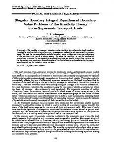
3.1 A square domain with Dirichlet boundary condition Fig. 1 shows the configuration of the generalized Laplace equation in a square domain (0, 1) × (0, 1) subject to the following Dirichlet boundary conditions: u( x1 , 0) = x1 + 2,

u( x1 , 1) = u(0, x2 ) = u(1, x2 ) = 2.

(3.2)

Its corresponding exact solution is ∞

2(−1)n+1 u ( x1 , x2 ) = 2 + ∑ sinh(nπ (1 − x2 )) sin(nπx1 ). nπ sinh(nπ ) n =1

(3.3)

The number of boundary nodes N used varies from 40 to 400. The boundary nodes are uniformly distributed along the boundary, except for four corner points. The interior point (0.5, 0.5) is chosen for the calculation of the constant c used in the inverse interpolation technique, as shown in Eq. (2.18). We here give the values of c for N = 100 and 200 in order to allow for checking of the possible recalculations by the interested readers (c = −0.2186 for N = 100 and c = −0.3923 for N = 200). Fig. 2 displays the relative error curve of the improved SBM at M = 120 field points uniformly distributed along the line x2 = 0.5 with 0.1 ≤ x1 ≤ 0.9, compared with those by using the ordinary SBM, RMM, MFS and BEM. For the MFS simulation, the distance d of he fictitious boundary away from the physical boundary is quantified by the unit s which is the interval spacing of nodes on the physical boundary. The BEM solutions are obtained using linear discontinuous boundary elements. A linear boundary element is adequate in this case because it can represent a straight line

552

W. Chen and Y. Gu / Adv. Appl. Math. Mech., 4 (2012), pp. 543-558

boundary exactly. It is stressed that the number of boundary nodes is all the same in the SBMs, RMM, BEM and MFS. It can be observed from Fig. 2 that the convergence trend of the improved SBM is better than those of using other methods. Particularly, when using 400 boundary nodes, the improved SBM is more accurate than the BEM by one order of magnitude, the ordinary SBM by two orders of magnitude and the RMM almost by three orders of magnitude. Namely, the present SBM formulation has the most fast convergence rate compared with other tested methods. In addition, we also note that the ordinary SBM has an oscillatory curve of relative errors and loses the stability when the boundary node number is larger than 200. In sharp contrast to the ordinary SBM, the improved SBM is of stably monotonic convergence with an increasing number of boundary nodes. In the MFS, the solution accuracy with the fictitious boundary d = s/2 deteriorates, while the MFS with d = 3s fictitious boundary gets more fast convergence rate in this case. This shows that the appropriate or optimal placement of the fictitious boundary in the MFS can result in a very accurate solution. However, unfortunately, it remains an open issue to find the appropriate fictitious boundary for complex problems.

3.2

A circular domain with Dirichlet boundary condition

As shown in Fig. 3, a circular domain of radius r = 2 is considered, which is an example used in [17]. Dirichlet boundary condition is imposed on the edge of the circle using the following analytical solution: u(r, θ ) = r6 cos(6θ )

(3.4)

in the polar coordinates (r, θ ). The number of boundary nodes N used varies from 100 to 1400. The boundary nodes are uniformly distributed along the boundary. The interior point (0.5, 0.5) is chosen for the calculation of the constant c used in the inverse interpolation technique. Again, we here give the values of c for N = 100 and 200 in order to allow for checking

Figure 1: A square domain with Dirichlet boundary condition.

W. Chen and Y. Gu / Adv. Appl. Math. Mech., 4 (2012), pp. 543-558

553

Figure 2: Relative error curves for the square domain, respectively, by using the improved and ordinary SBMs, the RMM, the BEM and the MFS.

Figure 3: A circle domain with Dirichlet boundary condition.

of the possible recalculations by the interested readers (c = 0.2380 for N = 100 and c = −0.9209 for N = 200). The numerical evaluation of the relative error is performed using M = 120 calculation points uniformly distributed on a circle with radius r = 1 and center at the origin. With the number of boundary nodes increases, Fig. 4 illustrates the relative error curves for different methods. Here, the BEM solutions are obtained using discontinuous quadratic elements since the quadratic element is ideal as it can approximate the geometry of curvilinear boundary with sufficient accuracy. Also, it is stressed that the number of boundary nodes is the same in the tested numerical methods. It can be observed from Fig. 4 that the improved SBM method performs better than other tested methods with an increasing number of boundary nodes. Particularly, when using 1400 boundary nodes, the improved SBM is more accurate than the ordinary SBM by one order of magnitude, the RMM and BDS by four orders of magnitude. In this case, we find that the solution accuracy and convergence rate of the improved SBM and the BEM are very close. But it is worthy noting that the SBM is inherently free of integration and mesh and far more computationally efficient, easier to program, and mathematically simple than the BEM.

554

W. Chen and Y. Gu / Adv. Appl. Math. Mech., 4 (2012), pp. 543-558

Figure 4: Relative error curves for the circle domain, respectively, by using the improved and ordinary SBMs, the RMM, the BDS and the BEM.

Figure 5: A multiply-connected domain with mixed boundary conditions.

3.3

A multiply-connected domain with mixed boundary conditions

Finally, the potential problem with multiply-connected domain subjected to the mixedtype boundary conditions is considered. A square domain (0, 3) × (0, 3) with a regular triangle hole is shown in Fig. 5 and the analytical solution is u( x1 , x2 ) = x12 − x22 + x1 x2 .

(3.5)

In this example, we suppose that the Dirichlet conditions are prescribed on the boundary of the square domain and the Neumann boundary conditions are prescribed on the boundary of the triangle domain. The number of boundary nodes N used varies from 150 to 3000. The boundary nodes are uniformly distributed along the boundary, except for seven corner points. The interior point (0.2, 0.2) is chosen for the calculation of the constant c used in the inverse interpolation technique. Again, we here give the values of c for N = 150 and 300 in order to allow for checking of the possible recalculations by the interested readers (c = −0.1882 for N = 150 and c = −0.1189 for N = 300). Fig. 6 displays the relative error curve of the improved SBM at M = 240 field points uniformly distributed along the square (0, 2.5) × (0, 2.5), compared with those by using the ordinary SBM, RMM, BEM and MFS. Again, the BEM solutions are obtained using liner discontinuous boundary elements. For the MFS solution, our experiments

W. Chen and Y. Gu / Adv. Appl. Math. Mech., 4 (2012), pp. 543-558

555

Figure 6: Relative error curves for the multiply-connected domain, respectively, by using the improved and ordinary SBMs, the RMM, the BEM and the MFS.

find that the fictitious boundaries having the same geometrical shape of the corresponding boundary are optimal. As in the first example, the distance d of the fictitious boundary away from the physical boundary is quantified by the unit s which is the interval spacing of nodes on the physical boundary. It can be observed from Fig. 6 that when the number of boundary nodes less than 2100, the BEM converges slightly faster than the improved SBM. However, the improved SBM outperforms the BEM as the number of boundary nodes increases, i.e., after 2100 boundary nodes. We can observe that the ordinary SBM has an oscillatory convergence curve of relative errors with the increase of the boundary node number. The present SBM remedies this drawback and performs stably with a fast convergent rate, indicating that the method works well with complicated domain problems. Compared with the RMM, the improved SBM is more accurate by about two orders of magnitude. In addition, we can see that when the number of boundary nodes less than 750, the MFS with d = s has the faster convergence rate than the improved SBM. However, with the increasing boundary nodes, the relative error curve of the MFS (d = s) oscillates severely, while the improved SBM remains steady and ultimately is more accurate than the MFS by one order of magnitude. It was also found that the MFS solution accuracy with the fictitious boundary d = s/2 dramatically deteriorates compared with the fictitious boundary d = s. This illustrates that the location of source nodes is vital to the accuracy and stability of the MFS solution.

4 Conclusions This paper proposed an improved formulation of singular boundary method to solve the Laplace problems subjected to Dirichlet, Neumann or mixed-type boundary conditions. The finite values of the origin intensity factors on the Neumann boundary condition have been extracted out and accurately evaluated by using the proposed desingularization technique without using sampling nodes and solution. The origin intensity factors on the Dirichlet boundary condition is calculated in a modified inverse interpolation technique without using sampling nodes. It is worthy of stressing that the new formulation circumvents troublesome sampling points, one of major

556

W. Chen and Y. Gu / Adv. Appl. Math. Mech., 4 (2012), pp. 543-558

problems, in the ordinary SBM formulation, while retaining all its merits being mathematically simple, easy-to-program, accurate, truly meshless and integration-free. In addition, the proposed new method avoids the controversy of the fictitious boundary in the MFS, the double-layer potentials used in the RMM and the expensive calculation of diagonal elements in both the MMFS and the BDS. In a summary of overall performances of our three numerical experiments, the present SBM is superior over the RMM, the BEM, the BDS and also the MFS in terms of accuracy and stability. The opening issues with the proposed improved SBM formulation are as follows. We need to examine the SBM with more complicated cases. The origin intensity factors on the Dirichlet boundary condition still need to be indirectly determined by the inverse interpolation technique via sample solution of problem of interest. A novel approach tackling this issue is now under intense study and the further results will be reported in a subsequent paper. The proposed improved SBM for 2D Laplace problems also offers great promise in the analysis of many other problems, including elasticity or Stokes flow problems. Some work along this line is already underway and will be reported in a subsequent paper.

Appendix: The detail derivations of Eq. (2.8) The null-fields of the boundary integral equations based on the direct method is [11, 28]: ∫ [

0=

Γ

u ∗ C ( xi , s )

] ∂u(s) ∂u∗ C ( xi , s) − u(s) dΓ(s), ∂ns ∂ns

xi ∈ ΩC ,

(A.1)

where the superscript (C ) denotes the exterior domain, s is the source point located on the physical boundary, xi is the field point. Substituting the simple solution u(s) = 1, ∂u(s)/∂ns = 0 into the Eq. (A.1), we can obtain the following equation: ∫ Γ

∂u∗ C ( xi , s) dΓ(s) = 0, ∂ns

xi ∈ ΩC .

(A.2)

When the field point xi approaches the boundary, we can discretize the Eq. (A.2) as follows: ∫ Γ

N ∂u∗ C ( xi , s) dΓ(s) = ∑ ∂ns j =1

∫ Γj

∂u∗ C ( xi , s) dΓ j (s) ∂ns

∂u∗ C ( xi , s j ) l j = 0, ∂ns j j =1 N

≈∑

xi , s j ∈ Γ,

(A.3)

W. Chen and Y. Gu / Adv. Appl. Math. Mech., 4 (2012), pp. 543-558

557

where l j is half distance of the source nodes s j−1 and s j+1 . When the distribution of boundary nodes is uniform, we are able to reduce the Eq. (A.3) to the following form: ∂u∗ C ( xi , s j ) = 0, ∑ ∂ns j j =1 N

xi ∈ Γ,

(A.4)

which is the Eq. (2.8) in the text of Section 2.1.

Acknowledgements The work described in this paper was supported by the National Basic Research Program of China (973 Project No. 2010CB832702), the National Science Funds for Distinguished Young Scholars of China (11125208), the R & D Special Fund for Public Welfare Industry (Hydrodynamics, Project No. 201101014) and Jiangsu Province Graduate Students Research and Innovation Plan (No. CXZZ11 0424).

References [1] A. K ARAGEORGHIS, Modified methods of fundamental solutions for harmonic and biharmonic problems with boundary singularities, Numer. Methods. Partial. Diff. Eq., 8 (1992), pp. 1–19. [2] G. FAIRWEATHER AND A. K ARAGEORGHIS, The method of fundamental solutions for elliptic boundary value problems, Adv. Comput. Math., 9 (1998), pp. 69–95. [3] C. S. C HEN , M. A. G OLBERG AND Y. C. H ON, The method of fundamental solutions and quasi-Monte-Carlo method for diffusion equations, Int. J. Numer. Methods Eng., 43 (1998), pp. 1421–1435. [4] C. S. C HEN AND G. R. L IU, Preface to: mesh reduction techniques-part I, Eng. Anal. Bound. Elem., 28 (2004), pp. 423–424. [5] Y. J. L IU , N. N ISHIMURA AND Z. H. YAO, A fast multipole accelerated method of fundamental solutions for potential problems, Eng. Anal. Bound. Elem., 29 (2005), pp. 1016–1024. [6] C. S. C HEN , H. A. C HO AND M. A. G OLBERG, Some comments on the ill-conditioning of the method of fundamental solutions, Eng. Anal. Bound. Elem., 30 (2006), pp. 405–410. [7] W. C HEN AND M. TANAKA, A meshless, integration-free and boundary-only RBF technique, Comput. Math. Appl., 43 (2002), pp. 379–391. [8] W. C HEN AND Y. C. H ON, Numerical investigation on convergence of boundary knot method in the analysis of homogeneous Helmholtz, modified Helmholtz and convection-diffusion problems, Comput. Methods. Appl. Mech. Eng., 192 (2003), pp. 1859–1875. [9] J. T. C HEN , M. H. C HANG , K. H. C HEN AND I. L. C HEN, Boundary collocation method for acoustic eigenanalysis of three-dimensional cavities using radial basis function, Comput. Mech., 29 (2002), pp. 392–408. [10] M. F OOLADI , H. G OLBAKHSHI , M. M OHAMMADI AND A. S OLEIMANI, An improved meshless method for analyzing the time dependent problems in solid mechanics, Eng. Anal. Bound. Elem., 35 (2011), pp. 1297–1302. [11] D. L. Y OUNG , K. H. C HEN AND C. W. L EE, Novel meshless method for solving the potential problems with arbitrary domain, J. Comput. Phys., 209 (2005), pp. 290–321. [12] D. L. Y OUNG , K. H. C HEN AND C. W. L EE, Singular meshless method using double layer potentials for exterior acoustics, J. Acoust. Soc. Am., 119 (2005), pp. 96–107.

558

W. Chen and Y. Gu / Adv. Appl. Math. Mech., 4 (2012), pp. 543-558

[13] A. H. D. C HENG AND D. T. C HENG, Heritage and early history of the boundary element method, Eng. Anal. Bound. Elem., 29 (2005), pp. 268–302. [14] W. S. H WANG , L. P. H UNG AND C. H. K O, Non-singular boundary integral formulations for plane interior potential problems, Int. J. Numer. Methods Eng., 53 (2002), pp. 1751–1762. [15] K. H. C HEN , J. T. C HEN AND J. H. K AO, Regularized meshless method for antiplane shear problems with multiple inclusions, Int. J. Numer. Methods Eng., 73 (2008), pp. 1251–1273. [16] B. S ARLER, Solution of potential flow problems by the modified method of fundamental solutions: formulations with the single layer and the double layer fundamental solutions, Eng. Anal. Bound. Elem., 33 (2009), pp. 1374–1382. [17] Y. J. L IU, A new boundary meshfree method with distributed sources, Eng. Anal. Bound. Elem., 34 (2010), pp. 914–919. [18] W. C HEN, Singular boundary method: a novel, simple, meshfree, boundary collocation numerical method, Chin. J. Solid. Mech., 30 (2009), pp. 592–599. [19] W. C HEN AND F. Z. WANG, A method of fundamental solutions without fictitious boundary, Eng. Anal. Bound. Elem., 34 (2010), pp. 530–532. [20] W. C HEN , Z. J. F U AND X. W EI, Potential problems by singular boundary method satisfying moment condition, Comput. Model. Eng. Sci., 54 (2009), pp. 65–85. [21] Y. G U , W. C HEN AND C. Z. Z HANG, Singular boundary method for solving plane strain elastostatic problems, Int. J. Solids Struct., 48 (2011), pp. 2549–2556. [22] M. A. G OLBERG, The method of fundamental solutions for Poisson’s equation, Eng. Anal. Bound. Elem., 16 (1995), pp. 205–213. [23] A. P OULLIKKAS , A. K ARAGEORGHIS , G. G EORGIOU AND J. A SCOUGH, The method of fundamental solutions for stokes flows with a free surface, Numer. Methods Partial Diff. Eq., 14 (1998), pp. 667–678. [24] C. S. C HEN , A. S. M ULESHKOV, M. A. G OLBERG AND R. M. M. M ATTHEIJ, A mesh-free approach to solving the axisymmetric Poisson’s equation, Numer. Methods Partial Diff. Eq., 21 (2005), pp. 349–367. [25] L. M ARIN, Regularized method of fundamental solutions for boundary identification in twodimensional isotropic linear elasticity, Int. J. Solids Struct., 47 (2010), pp. 3326–3340. [26] J.-H. Z HENG , M. M. S OE , C. Z HANG AND T.-W. H SU, Numerical wave flume with improved smoothed particle hydrodynamics, J. Hydrodyn. Ser. B, 22 (2010), pp. 773–781. [27] P. K. B ANERJEE, The Boundary Element Methods in Engineering, McGRAW-HILL Book Company Europe, 1994. [28] J. T. C HEN AND P. Y. C HEN, Null-field integral equations and their applications, in: Boundary Elements and Other Mesh Reduction Methods XXIX., WIT Press, Southampton, 2007, pp. 88–97.