An improved genetic algorithm for pipe network ... - Semantic Scholar

WATER RESOURCES RESEARCH, VOL. 32, NO.2, PAGES 449-458, FEBRUARY 1996

An improved genetic algorithm for pipe network optimization Graeme C. Dandy, Angus R. Simpson, and Laurence J. Murphy Department of Civil and Environmental Engineering, University of Adelaide, Adelaide, Australia

i

Abstract An improved genetic algorithm (GA) formulation for pipe network optimization has been developed. The new GA uses variable power scaling of the fitness function. The exponent introduced into the fitness function is increased in magnitude as the GA computer run proceeds. In addition to the more commonly used bitwise mutation operator, an adjacency or creeping mutation operator is introduced. Finally, Gray codes rather than binary codes are used to represent the set of decision variables which make up the pipe network design. Results are presented comparing the performance of the traditional or simple GA formulation and the improved GA formulation for the New York City tunnels problem. The case study results indicate the improved GA performs significantly better than the simple GA. In addition, the improved GA performs better than previously used traditional optimization methods such as linear, dynamic, and nonlinear programming methods and an enumerative search method. The improved GA found a solution for the New York tunriels problem which is the lowest-cost feasible discrete size solution yet presented in the literature.

Introduction Over the last 5 years a methodology for the application of genetic algorithms (GAs) to water distribution pipe network optimization has been developed [Murphy and Simpson, 1992; Dandy et al., 1993; Simpson et at., 1993; Murphy et al., 1993; Simpson et al., 1994]. Previous research has concentrated on developing a methodology for applying GAs to pipe network optimization using a simple genetic algorithm. This paper extends the earlier research by presenting an improved genetic algorithm formulation. There are three main changes to the simple GA that significantly enhance its performance and have been shown to result in substantial reductions in the cost of the optimized pipe network designs. The following features are incorporated in the improved genetic algorithm formulation: (1) variable power scaling of the fitness function, (2) an adjacency mutation operator, and (3) use of Gray codes. This paper gives an overview of the genetic algorithm technique by describing a simple GA and its application to pipe network optimization. Next, the features of the improved GA are described. The paper then describes the application of the improved GA to the New York City tunnels problem. Previous studies of the New York tunnels problem are reviewed. The performance of the improved GA formulation is then compared to the performance of the traditional GA formulation. Finally, the designs determined by the GA search are compared with the solutions of previous studies of the New York tunnels problem.

The Pipe Network Design Problem The optimal design of water distribution networks for gravity systems as addressed in this paper may be formulated as follows. For a given layout of pipes and a set of specified demand patterns at the nodes, find the combination of pipe sizes which gives the minimum material and construction cost subject to Copyright 1996 by the American Geophysical Union. Paper riumber 95WR02917. 0043-1397/96/95WR-02917$05.00

the following constraints: (1) Continuity of flow must be maintained at all junctions. (2) The head loss in each pipe is a known function of the flow in the pipe, its diameter, length, and hydraulic properties. (3) The algebraic sum of the head losses around each loop should equal zero. (4) Minimum and maximum pressure limitations at certain nodes in the network must be satisfied. (5) Minimum diameter requirements may be specified for certain pipes in the network.

Genetic Algorithms A genetic algorithm is a member of a class of search algorithms based on artificial evolution [Holland, 1975]. GAs simulate mechanisms of population genetics and natural rules of survival in pursuit of the ideas of adaptation. The GA search, sometimes with modifications to the simple GA formulation, has been shown to perform efficiently in a number of applications. This efficiency indicates the robustness of the search method that underlies the GA approach and the flexibility of the formulation itself [Goldberg, 1989]. In recent years a number of researchers have applied the genetic algorithm technique to certain aspects of the design of pipeline systems. Goldberg and Kuo [1987] applied the traditional GA to the optimization of the operation of a steady state serial gas pipeline consisting of 10 pipes and 10 compressor stations each containing 4 pumps in series. The objective in that study was to minimize power while supplying a specified flow and maintaining allowable pressures. Davidson and Goulter [1994] used GAs to optimize the layout of a branched rectilinear network, such as a rural natural gas or water distribution system. The optimal layout in that case was assumed to be the one of least length. The layout solutions were represented by blocks of binary code, and new GA operators of recombination and perturbation were introduced to reduce the number of infeasible solutions created by the traditional GA operators of crossover and mutation. Walters and Lohbeck [1993] studied the case of pipe networks with one demand pattern and no constraints on minimum pipe diameters. They showed that the GA effectively converges to near-optimal

449

450

DANDY ET AL.: GENETIC ALGORITHM FOR PIPE NETWORK OPTIMIZATION

Available Pipe Sizes and Pipe Costs for New York City Tunnels Duplication and Corresponding Codes as Examples of Genetic Algorithm (GA) Coding Schemes

Table 1.

Corresponding Coded Substrings Diameter, inches

Pipe Cost, $/foot

Binary

Gray

0 36 48 60 72 84 96 108 120 132 144 156 168 180 192 204

0 93.5 134.0 176.0 221.0 267.0 316.0 365.0 417.0 469.0 522.0 577.0 632.0 689.0 746.0 804.0

0000 0001 0010 0011 0100 0101 0110 0111 1000 1001 1010 1011 1100 1101 1110 1111

0000 0001 0011 0010 0110 0111 0101 0100 1100 1101 1111 1110 1010 1011 1001 1000

Note that 1 inch

=

25.4 mm and 1 foot

=

0.3048 m.

branched network layouts, as selected from a directed base graph which defines a set of possible layouts. In that study the nodal connectivity within the trial branch network solutions was represented by a string of code. Alternative GA coding schemes, induding a binary representation and an integer representation, were also investigated in that study. Walters and Cembrowicz [1993] extended these concepts using linear pro·gramming for the optimal selection of pipe sizes for branched pipe networks generated by a GA. The combination of GAs, graph theory, and linear programming was found by Walters and Cembrowicz [1993] to be the basis for an effective search for near-pptimal branched pipe network designs. Coded Strings

The genetic algorithm requires that the decision variables describing trial solutions to the pipe network design problem be represented by a unique coded string of finite length. This coded string is similar to the structure of a chromosome of genetic code. Consider a coded string consisting of 21 coded substrings each of 4 binary bits. This coded string of 84 binary bits may, for example, represent a design for a simple pipe network consisting of 21 pipes. Each 4-bit substring represents one of 16 possible choices of pipe size for one of the 21 pipes in the network. A selected mapping between the coded substrings and the design variables associates the artificial genetic code with a pipe network design. For example, Table 1 gives a mapping between coded substrings and actual pipe diameters for the New York tunnels problem considered later in this paper. Fitness of a Coded String

The fitness of a coded string representing a pipe network design is determined by both the pipe costs and the hydraulic performance of the pipe network design. The cost of the pipe network design is taken as the sum of (1) materials, construction, maintenance, and operation costs and (2) penalty costs (where the minimum pressure requirements are violated). A steady state hydraulic analysis of the pipe network design is performed to aSsess the hydraulic feasibility of the proposed

system. This hydraulic analysis involves the prediction of the flows in the pipes and hydraulic heads at the nodes in the pipe network under steady state conditions. The hydraulic analysis method adopted in this study uses the Newton-Raphson technique applied to the set of simultaneous nonlinear algebraic equations in terms of the unknown flow corrections around the loops. These are called the loop equations [Epp and Fowler, 1970]. Wood and Rayes [1981] demonstrated the reliability of this method. As hydraulic analysis is required for all new strings during the GA run, this can be computationally intensive. As part of this research, we have implemented sparse matrix techniques to ensure the hydraulic solver is as fast as possible.

A Simple Genetic Algorithm A brief description of the steps in using simple genetic algorithms for pipe network optimization is repeated here for completeness [Simpson et al., 1993]: 1. Generation of initial population. The GA randomly generates an initial population of coded strings representing pipe network solutions of population size N (typically N = 100 to 1000). Each bit position in the string takes on a value of either 1 or O. Each of the N strings of the random starting population represents a possible combination of pipe sizes and thus represents a different configuration of a pipe network. 2. Computation of network cost. The GA considers each of the N strings in the population in turn. It decodes each substring into the corresponding pipe size and computes the total material and construction cost. The GA determines the costs of each trial pipe network design in the current population. 3. Hydraulic analysis of each network. A steady state hydraulic network solver computes the heads and discharges under the specified demand patterns for each of the network designs in the population. The actual nodal pressures are compared with the minimum allowable pressure heads, and any pressure deficits are noted. 4. Computation of penalty cost. The GA assigns a penalty cost for each demand pattern if a pipe network design does not satisfy the minimum pressure constraints. The pressure violation at the node at which the pressure deficit is maximum is used as the basis for computation of the penalty cost. The maximum pressure deficit is multiplied by a penalty factor k (e.g., k = $5 million/foot of pressure head), which is a measure of the cost of a deficit of one unit of pressure head. 5. Computation of total network cost. The total cost of each network in the current population is taken as the sum of the network cost (step 2) plus the penalty cost (step 4). 6. Computation of the fitnesses. The fitness of the coded string is taken as some function of the total network cost. The GA computes the fitness for each proposed pipe network in the current population as the inverse of the total network cost from step 5. Two other forms of fitness function were tried; however, the use of the inverse was found to be the most effective in the GA search. 7. Generation of a new population using the selection operator. The GA generates new members of the next generation by a selection scheme. The probability of selection of string i, Pi' to go into the next generation of N members using a proportionate selection method is given by .


(1) where Ii is the fitness of string i (determined in step 6). 8. The crossover operator. Crossover is the partial exchange of bits between two parent strings to form two offspring strings. Crossover occurs with some specified probability of crossover Pc for each pair of parent strings selected in step 7. To perform one-point crossover, a crossover point is randomly selected along the strings. The crossover operator exchanges the bits after the crossover point between the two selected parent strings. 9. The mutation operator. Mutation occurs with some specified probability of mutation Pm for each bit in the strings which have undergone crossover. The bitwise complement mutation operator changes the value of the bit to the opposite value (i.e., 0 to 1 or 1 to 0). 10. Production of successive generations. The use of the three operators described above produces a new generation of pipe network designs using steps 2 to 9. The GA repeats the process to generate successive generations. The least cost. strings (e.g., the best 20) are stored and updated as cheaper cost alternatives are generated. Typically, a GA will evaluate between 100 and 1000 generations.

An Improved Genetic Algorithm Formulation The improved GA formulation was achieved by the combination of (1) variable exponent fitness scaling, (2) an adjacency mutation operator, and (3) Gray code representation. This order was found to be the order of significance of each feature in providing an improvement compared with the simple GA. Scaled Fitness of a Coded String Goldberg [1989] reported on fitness scaling mechanisms used to adjust the calculated raw fitness of strings in a population to maintain appropriate levels of competition between the strings. Gillies [1985] considered a power law form of fitness scaling, where the scaled fitness I; is some power of the raw fitness Ii given by (2). Gillies used a value of n = 1.005 in a machine vision application.

(2) The variable exponent n in (2) is used to modify the fitness function as part of the improved GA formulation. This is a crucial feature of the new improved GA formulation. The value of the exponent n is allowed to increase in steps as the GA run develops. The starting population of N strings is generated randomly and, as a consequence, this population and early generations are likely to contain diverse strings of genetic code. The average string fitness in the starting population will be relatively low, and the individual string fitnesses may vary significantly, and yet all of the strings may possess potentially valuable genetic information. A low value of the exponent n should be employed at the start of the GA run, for example, n = 1, so the GA can sort through the potential strengths of the ordinary strings in the early generations. A low value of n preserves some population diversity in the early generations. A larger value of the exponent n is not appropriate here since the GA search may be misguided by encouraging one extraordinary string to dominate the new populations. After a number of generations a large number of useful

451

string similarities are recognized and have become established. The value of the exponent n in the fitness function may be increased in steps during the intermediate generations. As the GA run progresses further, the highly fit string similarities that have evolved begin to dominate the populations. The strings are constructed of similar genetic code and their magnitudes of raw fitness may be very similar. A high value of the exponent n, say 3 or 4, is needed to accentuate the small differences in string fitness. The Adjacency Mutation Operator

An adjacency or creeping mutation operator has also been included in the improved GA formulation. Davis and .coombs [1987] and Coombs and Davis [1987] introduced an operator called "creep" into their study of the design of packetswitching communication networks. The coded strings were lists of communication link speeds that corresponded to links in the network, and creep altered selected link speeds upward or downward one or more steps in the list of allowable link speeds. The adjacency mutation operator presented here operates in a similar manner and is applied to complete decision variable substrings chosen randomly from the coded string. The adjacency mutation operator presented in this paper mutates the selected complete decision variable substring to an adjacent decision variable substring up or down the list of design variable choices. For example, the decision variable substring 0001 may be mutated up to 0010 (for binary coding) or mutated down to 0000. The substring 0000 may be mutated up to 0001 or may be left as 0000 since it cannot be mutated down. The adjacency mutations contrast with the traditional bitwise mutations that may or may not produce an adjacent substring. For example, the substring 0000 may be altered by a bitwise mutation to 1000, 0100, 0010, or 0001. The substrings 1000 and 0100 are very distant from 0000 in the substring list. Bitwise mutations with low probability and adjacency mutations were both used in the improved GA formulation. The adjacency mutation operator proposed here allows for the adjustment of conditional probabilities of upward and downward adjacency mutations (e.g.,Pd = 0.6 means there is a 60% probability of the adjacency mutation operator moving the pipe size from the current size to the next smaller size rather than the next larger size). The probability of the direction of the adjacency mutation can be biased in either direction. Gray Coding Scheme

Fundamental GA theory favors the use of coding schemes that are based on small alphabets. Small alphabets such as binary codes generate longer coded substrings and hence maximize the number of string similarities or schemata in a population of coded strings [Goldberg, 1990]. Traditionally, binary coding has been used to specify the mapping. However, the improved GA formulation uses a Gray code representation. Table 1 presents the alternative mappings between design variable choices and coded substrings for both binary and Gray coding schemes. The Gray code representation is such that adjacent decision variable coded substrings differ by one bit or are separated by a Hamming distance of 1 [Caruana and Schaffer, 1988]. For example, only 1 bit changes between neighboring substrings of 0011 and 0010 and 0110, etc. By comparison, adjacent substrings in binary coding may differ by any number of bits. For example, adjacent substrings 0111 and 1000 differ by 4 bits.

452


Figure 1.

New York City water supply tunnels.

This extreme Hamming distance of 4 is referred to as a Hamming cliff. Since similar genetic code represents adjacent design variable choices, the Gray codes ensure that trial network solutions that are nearby in the solution space are represented by similarly coded strings. Hollstien [1971] concluded Gray codes may be preferred to binary codes, since adjacent integers are only 1 bit distant and bitwise complement mutations cause less disruption of the solution. On the basis of experimental results, Bethke [1981] found Gray codes improved the performance of the GA and suggested the reason for this is that the Gray code maps Euclidean neighborhoods into Hamming neighborhoods. Caruana and Schaffer [1988] found the Gray codes to be better than or equivalent to binary coding for six functions tested, including the five functions considered by DeJong [1975]. Caruana and Schaffer [1988] concluded that by eliminating the Hamming Cliff of binary coding the Gray codes might improve the performance of the GA. The GA is blind to the mapping that occurs between a coded string and the set of design variables the string describes, and the GA process is not concerned with the method of evaluation of the coded string. Caruana and Schaffer suggested the GA may be misled by biases, such as a Hamming cliff, introduced by the mapping.

Case Study: The New York City Water Supply Tunnels Problem Schaake and Lai [1969] developed an optimization technique to determine the most economically effective design for

the proposed additions to the primary water distribution system of New York City. The system at that time was composed of a network of deep rock tunnels of large diameter (up to 204 inches, or 5182 mm). U.S. Customary units are used primarily in this paper to enable comparison against previously published results. Proposed expansions included the construction of gravity tunnels parallel to the existing tunnels to enable the system to meet increased water demands while maintaining minimum acceptable pressures. The New York City primary water supply tunnel system (as considered in the Schaake and Lai paper) is shown in Figure 1. The tunnel system is a gravity flow system that draws water (2017.5 feet 3 (s or 57,129.5 Lis) from the Hillview Reservoir at node 1. The primary tunnel system consisted of City Tunnels number 1 and number 2. City Tunnel number 1 extended from Hillview Reservoir to node 16 in Brooklyn by way of Manhattan. City Tunnel number 2 extended between Hillview Reservoir and Richmond down take by way of Queens. City Tunnel number 1 was constructed around 1920 and City Tunnel number 2 was constructed around 1940 [de Neufville et at., 1971]. The age of the City Tunnels and possible population increases with the associated increased water demands indicated the need for expansions to the existing network. A single demand pattern was considered for the improved tunnel system, and a corresponding minimum allowable total head was specified at each node, as given in Table 2. A hydraulic analysis for the projected demands applied to the existing tunnel system shows that nodes 16, 17, 18, 19, and 20 fall significantly below the required minimum total head [Bhave, 1985]. Nodes 1 to 15 have acceptable hydraulic grade line elevations. The lengths and diameters of the 21 existing pipes are given in Table 3. A Hazen-Williams roughness coefficient C = 100 is assumed for all existing and new pipes. The available tunnel sizes and associated costs considered for the New York City tunnels additions are presented in Table 1.

Table 2. Tunnels

Node

1 2 3 4 5 6 7 8 9 10

11 12

13 14 15 16 17 18 19 20

Nodal Data for New York City Water Supply

Demand, feet 3 /s

Minimum Total Head, feet

Reservoir 92.4 92.4 88.2 88.2 88.2 88.2 88.2 170.0 1.0 170.0 117.1 117.1 92.4 92.4 170.0 57.5 117.1 117.1 170.0

300.0 255.0 255.0 255.0 255.0 255.0 255.0 255.0 255.0 255.0 255.0 255.0 255.0 255.0 255.0 260.0 272.8 255.0 255.0 255.0

Note that 1 fooe/s = 28.36 Lis.


Table 3.

Pipe Data for the New York City Water Supply

Tunnels

Pipe

Start Node

End Node

Length, feet

Existing Diameter, inch

[1] [2] [3] [4] [5] [6] [7] [8] [9] [10] [11] [12] [13] [14] [15] [16] [17] [18] [19] [20] [21]

1 2 3 4 5 6 7 8 9 11 12 13 14 15 1 10 12 18 11 20 9

2 3 4 5 6 7 8 9 10 9 11 12 13 14 15 17 18 19 20 16 16

11600 19800 7300 8300 8600 19100 9600 12500 9600 11200 14500 12200 24100 21100 15500 26400 31200 24000 14400 38400 26400

180 180 180 180 180 180 132 132 180 204 204 204 204 204 204 72 72 60 60 60 72

Note that Hazen-Williams roughness coefficient C tunnels.

=

100 for all

Previous Studies Since the original work by Schaake and Lai [1969] a number of studies in pipe network optimization have considered the New York water supply tunnels as a case study to demonstrate the effectiveness of their respective techniques. The results of these studies are summarized in Table 4.

Table 4.

453

In the following review a continuous diameter design is an optimized set of pipe diameters that may take on any continuous real value. A discrete diameter design is a set of pipe diameters that are selected from a specified set of pipe sizes. A split pipe design may be derived from a continuous diameter design by decomposing a length of continuous diameter into partial lengths of the two adjacent discrete diameters (one smaller and one larger) to create a pipe with equivalent hydraulic properties. In the original work on the problem, Schaake and Lai [1969] used a linear programming approach to find the optimum pipe diameters for assumed values of the total head at each node. The decision variable for each pipe was its diameter raised to the power 2.63, thus leading to a set of linear constraints. The nonlinear terms in the objective function were approximated using piecewise linearization. No check was made to determine whether the assumed nodal heads led to an optimum solution overall. As shown in Table 4, the final solution obtained involves duplicating almost all pipes in the system at a cost of $78.09 million (all costs in this paper are given in 1969 dollars). As the minimum cost solution to a pipe network problem with one demand pattern and no constraints on minimum pipe diameters tends toward a branched system, it is expected that better solutions to the problem can be obtained by duplicating fewer tunnels. The optimization model of Quindry et at. [1981] was an extension of the linear programming approach used by Schaake and Lai [1969]. First, an optimal solution for an assumed set of nodal heads was obtained. The dual variables were then used to identify the relative changes required in the nodal heads so as to get the maximum rate of improvement in the objective function. The heads were adjusted and the linear program was rerun. This procedure was repeated until no

Comparative Designs for the New York Tunnels Problem Diameters of Duplicate Tunnels, inches QuindlY et al.

Gessler

Bhave

Morgan and Gaitlter [1985]

Kessler [1988]

Fujiwara and Khang [1990]

Pipe

Schaake and Lai [1969]

[1981]

[1982]

[1985]

(Slightly Infeasible")

(Clearly Infeasible")

(Clearly Infeasible*)

[1] [2] [3] [4] [5] [6] [7] [8] [9] [10] [11] [12] [13] [14] [15] [16] [17] [18] [19] [20] [21] Total cost, $M Diameter design

52.02 49.96 63.41 55.59 57.25 59.19 59.06 54.95 0.0 0.0 116.21 125.25 126.87 133.07 126.52 19.52 91.83 72.76 72.61 0.0 54.82 78.09 continuous

0.0 0.0 0.0 0.0 0.0 0,0 0.0 0.0 0.0 0.0 119.02 134.39 132.49 132.87 131.37 19.26 91.71 72.76 72.64 0.0 54.97 63.58 continuous

0 0 0 0 0 0 100 100 0 0 0 0 0 0 0 100 100 80 60 0 80 41.8 discrete

0.0 0.0 0.0 0.0 0.0 0.0 0.0 0.0 0.0 0.0 0.0 0.0 0.0 0.0 136.43 87.37 99.23 78.17 54.40 0.0 81.50 40.18 continuous

0 0 0 0 0 0 144 0 0 0 0 0 0 0 0 96 96 84 60 0 84 39.20 discrete

0.0 0.0 0.0 0.0 0.0 0.0 0.0 0.0 0.0 0.0 0.0 0.0 0.0 0.0 156.11 72.00 96.60 78.00 59.78 0.0 72.27 39.0 split pipe

0.0 0.0 0.0 0.0 0.0 0.0 73.62 0.0 0.0 0.0 0.0 0.0 0.0 0.0 0.0 99.01 98.75 78.97 83.82 0.0 66.59 36.1 continuous

$M, millions of dollars. *KYPIPES analysis.

454


Table 5. Runs Value of n

1 2 3

4

Variation of n for Improved GA Formulation Evaluation Number Interval

o < evaluations < 50,000

50,001 < evaluations < 100,000 100,001 < evaluations < 150,000 150,001 < evaluations < 200,000

further improvement was obtained. As shown in Table 4, the solution obtained involves no duplication of City Tunnel number 1. The total cost of the design was $63.58 million. Gessler [1982] used a partial enumeration technique and discrete pipe sizes to search a subset of the total solution space. He searched two separate regions of the solution space with consideration of the reinforcement of either City Tunnel number 1 or City Tunnel number 2. The lowest-cost discrete diameter solution obtained in each case was used as a starting solution for a gradient search technique that used continuous pipe sizes. The lowest-cost design involving the reinforcement of City Tunnel number 1 involved the duplication of only seven tunnels (Table 4) at a cost of $41.8 million. Bhave [1985] used a heuristic procedure based on the identification of an efficient branched configuration. In the method, nodal heads for the branched configuration were progressively adjusted so as to give the maximum reduction in system cost. The method identified City Tunnel number 2 (without tunnel [20]) as the branched configuration to be optimized. The optimal configuration (given in Table 4) involved the duplication of only six tunnels at a total cost of $40.18 million. Morgan and Goulter [1985] applied a linear programming approach coupled with a hydraulic network solver to the New York water supply tunnels problem. They used a split pipe approach in which the decision variables were the lengths of pipe of a specified diameter that replace the current size. Pipes may be increased or reduced in size or eliminated entirely (of course, the last two alternatives do not apply to the New York problem). After each iteration, hydraulic consistency was checked using the hydraulic network solver. The discrete pipe solution obtained by Morgan and Goulter is given in Table 4 and involves duplicating six tunnels at a cost of $39.20 million. The discrete pipe solution was found to be slightly infeasible but acceptable in terms of normal expected accuracies of simulation modelling. A split pipe solution with a cost of $38.9 million was also obtained. Kessler [1988] applied a decomposition technique consisting of two sub models [Kessler and Shamir, 1991] to the New York water supply tunnels problem. In the first submodel the heads at the nodes are fixed, and a minimum concave cost of flow algorithm is used to find the pipe flows. These are then fixed and the head variables are found in the second submodel using linear programming. The two sub models are solved interactively until convergence is achieved (which usually occurs after two iterations). It can be shown that a local optimum is obtained. A split pipe solution with a cost of $39.0 million was obtained. This is shown to be clearly infeasible later in this paper. Fujiwara and Khang [1990] used a two-phase decomposition method that combined the methods of Alperovits and Shamir [1977], Quindry et al. [1981], and Mahjoub[1983]. In the first phase a nonlinear programming gradient method was used to find the optimum head loss in each pipe (and hence the pipe

diameters) for an assumed set of flows. A correction was then applied to the assumed flow in each loop using the Lagrange multipliers associated with the previous solution. This process was continued until it converged on a local optimum. In the second phase the nodal heads obtained at the end of the first phase were fixed. A nonlinear optimization model was run that found the optimum flow in each pipe for these nodal heads. This gave a new local optimum that could be used to restart the first phase. Iteration occurred between the two phases in such a way as to obtain a better local optimum solution. Fujiwara and Khang [1990] proposed a continuous diameter pipe solution with a cost of $36.1 million, but this design is shown later in the paper to be clearly infeasible.

Genetic Algorithm Optimization The simple genetic algorithm formulation and the improved genetic algorithm formulation developed in this paper were both applied to the New York City tunnels network design problem. A 4-bit binary coded substring permits representation of 16 discrete alternative choices for a design variable. Since there are 21 existing pipes in the New York City network that may be duplicated, the coded strings representing a trial pipe network design are constructed of 84 binary bits (21 by 4-bit coded substrings). The result is a vast solution space of 1621 or 284 (= 1.9343 X 1025 ) different pipe network designs. The variable power scaling of the fitness function given in (3) is an important element of the improved GA. The exponent n was chosen as n = 1 for the simple GA runs. The exponent n was allowed to vary throughout the improved GA runs, as shown in Table 5.

J; =

(l/costy'

(3)

where J; is the scaled fitness of string i and cost; is the sum of all costs for string i (including penalty costs). The GA parameters chosen for the simple GA runs (T1 to T5) and improved GA runs (11 to IS) are given in Table 6. The GA parameters chosen for the improved GA runs are identical except that the adjacency mutation operator was not employed in the traditional GA runs. The GA runs were allowed 200,000 evaluations of different designs. This number of designs is only a relatively small fraction of the total solution space. Each GA run used approximately 50 min of central processing unit time on a Sun Sparc 1+ Station (running with the operating system SunOS 4.1) for the 200,000 function evaluations. A considerable proportion of this time is for the hydraulic analysis of each of the designs. Crossover occurs with a specified probability Pc, which is a GA parameter that may be varied. A value of Pc = 0.5 and a population size of N = 100 imply that approximately 50 (i.e., Pc' N) of the 100 coded strings in the new population will be created by crossing over two strings from the previous generation. The other 50 or so strings pass to the new generation without being crossed over. GA researchers [DeJong, 1975; GreJenstette, 1986; Goldberg, 1989] have suggested good performance of the GA may be obtained using high crossover probabilities (Pc = 0.5 to 1.0). Bitwise complement mutation should occur with low probability (Pm = 0.001 to 0.05). A value of Pm = 0.01 implies that approximately 1 bit in every 100 bits crossed over is mutated. Since the string length is 84 bits for the New York problem, with a value ofp", = 0.01, on the average, 42 bits will be mutated from 50 strings crossed


Table 6.

455

GA Parameter Values Traditional (T)/Improved (I) GA Runs GA Parameters

TlIl1

T2/I2

T3/I3

T4/I4

T5/I5

Population size, N Number of generations Number of evaluations Probability of crossover, Pc Probability of bitwise mutation, Pm Probability of adjacency mutation, P a Conditional probability of downward adjacency mutation, p" Pressure violation penalty multiplier, k ($M/foot)

500 800/534 200,000 0.5 0.01 0.0/0.5 0.0/0.5

200 1000 200,000 1.0 0.01 0.0/1.0 0.0/0.6

200 1000 200,000 1.0 0.01 0.0/1.0 0.0/0.6

100 2000 200,000 1.0 0.01 0.0/1.0 0.0/0.6

100 2000 200,000 1.0 0.005 0.0/0.5 0.0/0.6

12.5

10.0

15.0

10.0

5.0

over to form a new population. A high probability of crossover (Pc = 1.0) and a low probability of bitwise mutations (Pm = 0.01) are employed for most of the GA runs. An adjacency mutation occurs when a string for the new generation is selected with a specified probability P a. Every string for the new generation is subject to an adjacency mutation when a value of P a = 1.0 is used. A coded decision variable substring from among those which form the string is selected randomly. It is replaced by the adjacent decision variable substring down the substring list (toward 0000) with the conditional probability of a downward adjacency mutationp". Otherwise it is replaced with the adjacent decision variable substring up the list. A value of P d = 0.6 indicates a slight bias in the direction of a downward adjacency mutation or to the next smallest pipe rather than to the next largest pipe. An evaluation of a coded string is required for every new string created in a generation when an old string is altered by crossover and/or by bit or adjacency mutation. The expected number of generations for a given number of evaluations can be computed by considering the expected number of new strings created in a new population. It is given by the following equation:

Ng

=

E N~[l:-_--O-:(l:---p-c-:-)(=l---P-a=)]

(4)

where N g is the expected number of generations for the evaluation of E new strings. The denominator in (4) is the expected number of new strings per generation. It should be noted that crossover and adjacency mutation occur independently, whereas bit mutation is only possible for strings which undergo crossover. The random number generator seed producing the initial generation of strings was held constant for all the GA runs. This will produce the same sequence of random numbers and

Table 7.

generate the same starting population of designs. Generation of the same starting population is useful for the comparison of the GA formulations and combinations of the GA parameters. The pressure violation penalty multiplier k is the cost of a hydraulic grade line violation per foot of pressure head deficit. A particular level of the penalty multiplier sets the severity of the penalty costs imposed. The selected value of the penalty multiplier must produce penalty costs such that near-optimal infeasible solutions cost slightly more than the optimal solution. The optimal solution is not usually known, and an appropriate value of the pressure violation penalty multiplier differs from one problem to the other. As a result, some trial and error adjustment of the pressure violation penalty multiplier is necessary. The numbers of infeasible network solutions present in the search and the feasibility of the lowest-cost network solutions determined by the search should provide an indication of the suitability of the chosen value of the pressure violation penalty multiplier. A value of k = $5.0 million/foot generated many low-cost marginally infeasible network designs. Although the selection of the parameters for the genetic algorithm model requires some judgement, the authors have optimized 14 networks ranging in size from 14 to 260 pipes and have found that the results obtained are relatively insensitive to these parameters. The lowest-cost feasible pipe network designs determined by the five simple GA formulations and the five improved GA formulations are given in Table 7. The improved GA runs achieve a minimum cost feasible design for $38.80 million. This design is the lowest-cost feasible discrete pipe design identified in the literature. The evaluation numbers at which the lowest-cost designs were found are also given in Table 7. Figure 2 shows a plot of the best of generation costs against evaluation numbers for the traditional GA run T1 and the

Results of the GA Runs Simple GA Runs

Improved GA Runs

GARun

Lowest-Cost Feasible Design, $M

Evaluation Number

T1* T2 T3 T4 T5

41.93 51.07 45.07 48.23 40.33

199,250 163,800 121,600 128,600 158,000

*Plots are given in Figures 2 and 3.

GARun 11*

12 13

14 IS

Lowest-Cost Feasible Design, $M

Evaluation Number

38.80 39.06 38.80 39.06 39.17

96,750 137,400 151,400 145,700 187,700

456


110.0

New York City Water Supply Tunnels

New York City Water Supply Tunnels

(see Table 6 for all GA ammeter values)

(see Table 6 for all GA ammeter values) 180.0

g ::J. .§

90.0

~

§ c

70.0

0

.~ :l,

11

PO

50.0

20.0+---,--~~~~-~~-~-~~--l

30.0+-~-~-~~-~~-~-~~--,-l

o

40000

80000

120000

160000

o

200000

40000

80000 120000 Number of Evaluations

Number of Evaluations

160000

200000

Figure 2. Best of generation costs for simple genetic algorithm (GA) run Tl and improved GA run I1.

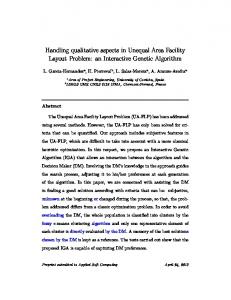
Figure 3. Average generation costs for simple GA run Tl and improved GA run I1.

equivalent improved GA run I1. Figure 3 shows a plot of the average generation costs against evaluation numbers for Tl and I1. A similar decreasing cost with generation characteristics is exhibited by Tl and I1 up to about 40,000 evaluations. Beyond this point, the improved GA formulation I1 can be seen to display superior performance and to generate solutions with significantly lower costs. The five least-cost feasible genetic algorithm designs and three infeasible genetic algorithm designs identified by any of the improved GA formulations are presented in Table 8. The corresponding total hydraulic heads at nodes 16, 17, and 19 for the eight GA designs are shown in Table 9. The lowest-cost feasible GA design has a cost of $38.80 million. Three feasible discrete pipe networks have been identified by the improved GA that are lower in cost ($38.80, $39.06, and $39.17 million) than the Morgan and Goulter [1985] network is at $39.20 million. Table 10 shows the hydraulic heads at the three critical

nodes for the previous designs. The acceptability of solutions is also related to the relative accuracy of network simulators. A solution may be regarded as infeasible for a "crisp" violation of the pressure constraints; however, it may be quite acceptable on a "fuzzy" basis. The Morgan and Goulter [1985] design is seen to be slightly infeasible. However, the pressure head violations are so small that the solution could be considered to be a valid feasible solution to the problem. The hydraulic analysis was carried out using the hydraulic network solver developed for this study. Similar results were obtained using the KYPIPES Computer Program. The GA designs shown in Table 8 belong to one of two groups of designs. The first group of designs duplicates pipe [7] in City Tunnel number 1, while the other group of designs duplicates pipe [15] at the upstream end of City Tunnel number 2. These same results also indicate pipes [16], [17], [18], [19], and [21] require duplication.

Table 8. The Least-Cost Improved GA Network Designs (Diameters of Duplicate Pipes in Inches) Feasible Designs

Infeasible Designs

Pipe

GA 1

GA2

GA3

GA4

GA5

GA6

GA 7

GA8

[1] [2] [3] [4] [5] [6]

0 0 0 0 0 0 0 0 0 0 0 0 0 0 120 84 96 84

0 0 0 0 0 0 144 0 0 0 0 0 0 0 0 96 108

0 0 0 0 0 0 156 0 0 0 0 0 0 0 0 96 96 84

0 0 0 0 0 0 0 0 0 0 0 0 0 0 120 84 108

0 0 0 0 0 0 0 0 0 0 0 0 0 0 108 96 96 84

0 0 0 0 0 0 0 0 0 0 0 0 0 0 96 96 96 84

0 0 0 0 0 0 84 0 0 0 0 0 0 0 0 96 96 84

0 0 0 0 0 0 0 0

0 0 0 0 0 0 96 96 84 72

[7]

[8] [9] [10] [11] [12] [13] [14] [15] [16] [17] [18] [19] [20] [21] Total Cost $M

0

72

72 72

72

72

72

0

0

0

0

0

0

0

72

72

72

72

72

72

72

72

38.80

39.06

39.17

39.22

39.28

38.52

36.19

33.62

72

72 72

0

457


Table 9.

Hydraulic Heads for GA Designs Minimum Heads at the Three Most Critical Nodes, feet

Minimum Required Head, feet Node 16 260.0 Excess Node 17 272.8 Excess Node 19 255.0 Excess Cost, $M

Feasible Designs

Infeasible Designs

GA 1

GA2

GA3

GA4

GA5

GA6

GA 7

GA8

260.52 +0.52

260.01 +0.01

260.08 +0.08

260.52 +0.52

260.23 +0.23

259.95 -0.05*

259.48 -0.52*

258.99 -1.01 "

272.86 +0.06

272.82 +0.02

272.88 +0.08

272.86 +0.06

273.02 +0.22

272.75 -0.05*

272.28 -0.52*

271.79 -1.01 *

255.71 +0.71 38.80

255.71 +0.71 39.06

255.04 +0.04 39.17

256.43 +1.43 39.22

255.39 +0.39 39.28

255.10 +0.10 38.52

254.50 -0.50* 36.19

254.07 -0.93* 33.62

"A negative value indicates the pressure constraint is violated.

The infeasible GA designs in Table 8 demonstrate substantial cost savings for some small violations of the pressure head constraints. Infeasibility may be acceptable in some circumstances, particularly if. a small hydraulic head deficiency is accompanied by large cost savings. The GA 8 design represents a cost saving of about $5.17 million (13.3%) compared with the lowest-cost feasible design. This may be an acceptable low-cost design with a hydraulic head deficiency of approximately 1 foot at nodes 16, 17, and 19. Infeasible designs become more prominent in the GA search when the pressure violation penalty cost multiplier is smaller. The design proposed by Fujiwara and Khang [1990] was claimed to be the lowest-cost published design solution to the New York City tunnels problem, but it is actually infeasible with the heads at nodes 16, 17, and 19 falling below the minimum allowable values. Thus the GA 1 design with a cost of $38.80 million is the lowest-cost, feasible, discrete diameter design for the New York City water tunnels problem to date.

Summary and Conclusions An improved genetic algorithm formulation for pipe network optimization has been presented in this paper. The improved GA formulation features (1) variable power scaling of the fitness function, (2) an adjacency mutation or creep operator, and (3) the use of Gray codes. The pipe network designs are represented by coded strings constructed using a binary

\,

Table 10.

alphabet. The variable exponent used to modify raw fitness values helps to maintain competitiveness throughout the GA search. In the early generations a low value of the exponent n overlooks small differences in string fitness, and this helps to preserve population diversity and allows for global exploration of the solution space. In the later generations, where highly fit (i.e., highly desirable) elements of the solution become more clearly evident, a high value of the exponent n emphasizes small differences in string fitness, and thIS helps to concentrate the search on the best regions of the solution space. The adjacency mutations change complete decision variable coded substrings to adjacent coded substrings in the list of design variable choices. The adjacency mutations are subtle disruptions of the code which permit local exploration of the solution space. The coded substrings which form the string are mapped to design variable choices, such as pipe diameters, by a Gray coding scheme. Gray codes are such that similar codes represent consecutive design variable choices, and therefore similarly coded strings represent designs nearby in the solution space. The performance of the simple and improved genetic algorithm formulations applied to the New York City tunnels problem was investigated. In addition, the results have been compared to solutions obtained previously in the literature using other techniques. Previously, the results by Fujiwara and Khang

Hydraulic Heads for Previous Designs Using the Hydraulic Network Solver Developed in This Research Minimum Heads at the Three Most Critical Nodes, feet

Allowable Head, feet Node 16 260.0 Excess Node 17 272.8 Excess Node 19 255.0 Excess Cost, $M

Schaake and Lai [1969]

QuindlY et al. [1981]

Gessler [1982]

Bhave [1985]

Morgan and Goulter [1985] (Infeasible)

Kessler [1988] (Infeasible)

Fujiwara and Khang [1990] (Infeasible)

261.02 +1.02

260.97 +0.97

260.32 +0.32

260.84 +0.84

261.56 +1.56

258.51 -1.49*

259.30 -0.70'

273.81 +1.01

273.66 +0.86

273.10 +0.30

273.38 +0.58

272.79 -0.01'

273.04 +1.04

272.26 -0.54*

256.14 +1.14 78.09

256.04 +1.04 63.58

255.86 +0.86 41.8

255.96 +0.96 40.18

254.99 -0.01* 39.20

255.22 +0.22 39.0

254.24 -0.76* 36.1

*A negative value indicates the pressure constraint is violated.

458


[1990] were considered to be the lowest-cost solution; however, it has been shown that their solution is, in fact, infeasible. The improved genetic algorithm produces significantly lower cost solutions than the simple genetic algorithm. The improved GA technique has identified three discrete diameter designs for the New York City tunnels problem with lower costs than feasible networks identified by any other technique in the literature. The lowest-cost feasible discrete pipe solution from the improved GA has a cost of $38.80 million. One significant advantage of the GA technique is that a range of solutions is produced by the GA such that the decision maker can choose between similarly priced alternatives. Some other criteria may then be used to decide which alternative is selected.

Notation cost; cost of the design represented by string i. E number of new evaluations. Ii raw fitness of string i. I: scaled fitness of string i. k pressure violation penalty multiplier ($/unit of hydraulic head). n variable exponent in fitness function. N population size. N g expected number of generations for the evaluation of E new strings. Pi probability of selection of string i. Pa probability of adjacency mutation. Pc probability of crossover. P d conditional probability of downward adjacency mutation. p;" probability of random bitwise mutation. Acknowledgments. This research work was supported by an Australian Research Council grant in 1992 and 1993. This support is gratefully acknowledged. The comments received from the referees were very useful in improving this paper. Their contributions are acknowledged.

References Alperovits, A., and U. Shamir, Design of optimal water distribution systems, Water Resour. Res., 13(6), 885-900, 1977. Bethke, A. D., Genetic algorithms as function optimizers, doctoral dissertation, 129 pp., Dep. of Comput. and Commun. Sci., Univ. of Mich., Ann Arbor, 1981. Bhave, P. R., Optimal expansion of water distribution systems, J. Environ. Eng. N. Y., 111(2),177-197,1985. Caruana, R. A., and J. D. Schaffer, Representation and hidden bias: Gray vs. binary coding for gcnctic algorithms, paper presented at Fifth International Conference on Machine Learning, Univ. of Mich., Ann Arbor, 1988. Coombs, S., and L. Davis, Genetic algorithms and communication link speed design: Constraints and operators, Genetic Algorithms and their Applications: Proceedings, Second International Conference on Genetic Algorithms, edited by J. J. Grefenstett, pp. 257-260, Lawrence Erlbaum, Hillsdale, N.J., 1987. Dandy, G. C., A. R. Simpson, and L. J. Murphy, A review of pipe network optimization techniques, in Proceedings of Watercomp '93, Melbourne, Australia, March/Aplil, Nat!. Con! Pub!. Inst. Eng. Aust., 9312, 373-383, 1993. Davidson, J. W., and I. C. Goulter, Evolution program for the design of rectilinear branched distribution systems, J. Comput. Civ. Eng., 9(2), 112-121, 1995. Davis, L., and S. Coombs, Genetic algorithms and communication link speed design: Theoretical considerations, Genetic AlgO/ithms and their Applications: Proceedings, Second International Conference on

Genetic Algorithms, edited by J. J. Grefenstett, pp. 252-256, Lawrence Erlbaum, Hillsdale, N.J., 1987. Dejong, K. A., An analysis of the behaviour of a class of genetic adaptive systems, Diss. Abstr. Int. B, 136(10), 5140, 1975. de Neufville, R., J. Schaake, and J. Stafford, Systems analysis of water distribution networks, f. Sanit. Eng. Div. Am. Soc. Civ. Eng., 97(SA6), 825-842, 1971. Epp, R., and A. G. Fowler, Efficient code for steady-state flows in networks,J. Hydrau!. Div. Am. Soc. Civ. Eng., 96(HY1), 43-56, 1970. Fujiwara, 0., and D. B. Khang, A two-phase decomposition method for optimal design of looped water distribution networks, Water Resour. Res., 26(4),539-549,1990. Gessler, J., Optimization of pipe networks, paper presented at International Symposium on Urban Hydrology, Hydraulics and Sediment Control, Univ. of Kentucky, Lexington, 1982. Gillies, A. M., Machine learning procedures for generating image domain feature detectors, doctoral dissertation, Univ. of Mich., Ann Arbor, 1985. Goldberg, D. E., Genetic Algorithms in Search, Optimization and Machine Learning, 412 pp., Addison-Wesley, Reading, Mass., 1989. Goldberg, D. E., Real-coded genetic algorithms, virtual alphabets, and blocking, IlUGAL. Rep. 90001, 18 pp., Dep. of General Eng., Univ. of Ill., Urbana-Champaign, 1990. Goldberg, D. E., and C. H. Kuo, Genetic algorithms in pipeline optimization, f. Comput. Civ. Eng., 1(2), 128-141, 1987. Grefenstette, J. J., Optimization of control parameters for genetic algorithms, IEEE Trans. Syst. Man Cybern., 16(1), 122-128, 1986. Holland, J. H., Adaptation in Natural and Artificial Systems, Univ. of Mich. Press, Ann Arbor, 1975. Hollstien, R. B., Artificial genetic adaptation in computer control systems, Diss. Abstr. Int. B, 32(3), 1510, 1971. Kessler, A., Optimal design of water distribution networks using graph theory techniques (in Hebrew), doctoral thesis in civil engineering, 142 pp., Technion, Israel Inst. of Techno!., Haifa, 1988. Kessler, A., and W. Shamir, Decomposition technique for optimal design of water supply networks, Eng. Optim., 17, 1-19, 1991. Mahjoub, Z., Contribution a l'etude de l'optimization des reseaux mailles, doctoral thesis, pp. 51-142, !'Inst. Nat!. Poly tech., de Toulouse, France, 1983. Morgan, D. R., and I. C. Goulter, Optimal urban water distribution design, Water Resour. Res., 21(5),642-652,1985. Murphy, L. J., and A. R. Simpson, Pipe optimization using genetic algorithms, Res. Rep. 93, p. 95, Dep. of Civ. Eng.; Univ. of Adelaide, S. Aust., June 1992. Murphy, L. J., A. R. Simpson, and G. C. Dandy, Design of a network using genetic algorithms, Water, 20, 40-42, 1993. Quindry, G., E. D. Brill, and J. C. Liebman, Optimization of looped water distribution systems, f. Environ. Eng. Div. Am. Soc. Civ. Eng., J07(EE4), 665-679, 1981. Schaake, J. c., and D. Lai, Linear programming and dynamic programming applications to water distribution network design, Rep. 116, Hydrodyn. Lab., Dep. of Civ. Eng., MIT, Cambridge, Mass., 1969. Simpson, A. R., L. J. Murphy, and G. C. Dandy, Pipe network optimization using genetic algorithms, paper presented at ASCE, Water Resources Planning and Management Specialty Conference, Am. Soc. Civ. Eng., Seattle, Wash., May, 1993. Simpson, A. R., G. C. Dandy, and L. J. Murphy, Genetic algorithms compared to other techniques for pipe optimization, J. Water Resour. Plann. Manage. Div. Am. Soc. Civ. Eng., 120(4), 423-443, 1994. Walters, G. A., and R. G. Cembrowicz, Optimal design of water distribution networks, in Water Supply Systems: State of the Art and Future Trends, edited by E. Cabrera and F. Martinez, Comput. Mech., Southampton, England, 1993. Walters, G. A., and T. Lohbeck, Optimal layout of tree networks using genetic algorithms, Eng. Optim., 22, 47-48, 1993. Wood, D. J.,and A. M. Rayes, Reliability of algorithms for pipe network analysis, J. Hydrau!. Div. Am. Soc. Civ. Eng., J07(HY10), 1145-1161, 1981. G. C. Dandy, L. G. Murphy, and A. R. Simpson, Department of Civil and Environmental Engineering, University of Adelaide, Adelaide, SA 5005, Australia. (e-mail: [email protected];lmurphy@ civeng.adelaide.edu.au; [email protected]) (Received June 13, 1995; revised September 12, 1995; accepted September 20, 1995.)