An Improved L-Shaped Method for Solving Process Flexibility Design ...

Hindawi Publishing Corporation Mathematical Problems in Engineering Volume 2016, Article ID 4329613, 15 pages http://dx.doi.org/10.1155/2016/4329613

Research Article An Improved L-Shaped Method for Solving Process Flexibility Design Problems Huasheng Yang,1 Jatinder N. D. Gupta,2 Lina Yu,1,3 and Li Zheng1 1

Department of Industrial Engineering, Tsinghua University, Beijing 100084, China University of Alabama in Huntsville, Huntsville, AL 35899, USA 3 Logistics Engineering and Simulation Laboratory, Graduate School at Shenzhen, Tsinghua University, Shenzhen 518055, China 2

Correspondence should be addressed to Huasheng Yang; [email protected] Received 2 March 2016; Revised 17 July 2016; Accepted 21 July 2016 Academic Editor: Xiangyu Meng Copyright © 2016 Huasheng Yang et al. This is an open access article distributed under the Creative Commons Attribution License, which permits unrestricted use, distribution, and reproduction in any medium, provided the original work is properly cited. Process flexibility, where a plant is able to produce different types of products, is introduced to mitigate mismatch risk caused by demand uncertainties. The long chain design proposed by Jordan and Graves in 1995 has been shown to be able to reap most benefits of full-flexibility structure (where each plant is able to produce all products) in balanced systems (where the numbers of products and plants are equal). However, when systems are not balanced or asymmetric or when response dimension is taken into consideration, long chain design may not be the best configuration. Therefore, this paper models the process flexibility design problem in more general settings. The paper considers both balanced and unbalanced systems with asymmetric plants considering response dimension. The problem is formulated as a two-stage stochastic program which is solved by an adapted L-shaped method, combining it with several enhancements. To the best of our knowledge, this is the first time L-shaped method is used to solve the process flexibility design problem. The effectiveness and efficiency of the proposed method and enhancements are evaluated. Finally, the comparison between design methods proposed in this paper and in existing literature shows the superiority of the former.

1. Introduction Demand for products or services has become more volatile and unpredictable due to seasonal fluctuations (see [1]), price fluctuations, or competitor uncertainties. In such an environment, matching capacitated supply and demand is vital for manufacturing companies and service centers. However, traditional strategies such as increasing supply capacities or inventories do not perform well (see [2–4]). A new operation strategy, namely, process flexibility, is introduced to mitigate such mismatch risk caused by uncertainties (see [5, 6]). Process flexibility, also known as “mixed flexibility” and “manufacturing flexibility,” is defined as the ability “to build different types of products in the same plant or production facility at the same time” in [7]. Without adequate flexibility, capacity-demand mismatch would occur (see [2, 8]), which might further hurt firms’ performances. Such an example could be found in [9]. Because of the economic crisis and high gasoline prices in 2008, overall vehicle sales declined and consumers preferred buying small or new energy-efficient

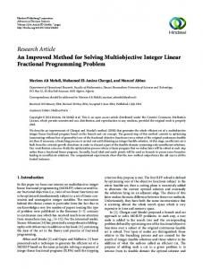
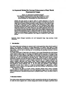
cars instead of pickup trucks or SUVs. Consequently, many automakers in Detroit without process flexibility suffered severe losses. Conversely, because of their ability to produce different vehicle models in at least one plant, Honda and Toyota survived and even gained in increase in their market share. Although flexibility is an effective way to hedge uncertainties, it is costly to implement. Motivated by their work at General Motors, Jordan and Graves [7] introduced the concepts of limited flexibility (i.e., a plant produces only a few types of products, also called “partial flexibility” or “sparse flexibility”) and chaining. They found that limited flexibility can reap most benefits of full flexibility when configured to chain products and plants together to the greatest extent possible, which is called long chain design. To make things simple, the term plant is used to refer to resource throughout this paper. Figure 1 illustrates three different kinds of flexibilities: dedicated design where each plant can produce only one product, the long chain design where each plant can

2 Plant

Mathematical Problems in Engineering Product

Dedicated

Long chain design

Total flexibility

Figure 1: Different types of flexibilities.

and only can produce two products, and total flexibility where each plant can produce all products. Because of the costly investment of flexibility and high performance of the long chain design, it has attracted much attention from both academicians and practitioners. However, it performs well in special settings such as in balanced and symmetric systems and when only demand shortfall is taken into consideration. Recently, several research works found that the long chain design does not perform in the best way when settings change. For balanced systems, Mak and Shen [2] numerically showed that long chain is not the optimal design under conditions with high or low demand variability, and D´esir et al. [10] showed that the optimal structure among designs with at most 2𝑛 arcs need not be the long chain if there is no connection restriction. For unbalanced systems where the numbers of resources and demands are not equal, Deng and Shen [9] proposed an alternative better design. In addition, in practice managers care more about the cost of flexibility. This means that, besides range dimension, response dimension is another important and practical dimension for process flexibility. Chou et al. [11] studied such a problem and argued that response dimension rather than range dimension should come first when resource is limited. When cost parameters are not perfectly flexible, Mak and Shen [2] found that the long chain design does not always perform in the best way. Legros et al. [12] claimed to have the same findings in the study of asymmetric call center systems. Therefore, in order to implement process flexibility in a practical unbalanced and asymmetric system with nonhomogeneous cost parameters, it requires further exploration to solve the process flexibility design (PFD) problems. This paper formulates the PFD problem with more general settings, including nonhomogeneous demand/cost and unbalanced system without assuming symmetric capacities as a two-stage stochastic programing problem. The model is based on the recent work of [2, 8]. Contrary to developing heuristic algorithms, this paper adapts a widely used method applied in stochastic programing, namely, L-shaped method, to solve the PFD problem. To the best of our knowledge, this is the first time L-shaped method is used to solve PFD problem. In order to obtain high solution quality and computational efficiency, this study further explores enhancements to speed up the algorithm. Results of numerical experiments show that the long chain design is not always the best configuration

although the optimal design is still sparse. Finally, the proposed design method is compared with existing heuristic methods in the context of both balanced and unbalanced systems. The comparison results show the superiority of the proposed method in this paper. The rest of the paper is organized as follows. Literature related to PFD and L-shaped method is reviewed in Section 2. Section 3 describes the problem and formulates models for the PFD problem. Following that, in Section 4, the basic Lshaped method adapted for our problem is developed and a set of enhancement strategies to speed up the computations is discussed. The effectiveness and efficiency of the adapted Lshaped method and the enhancement strategies are explored in Section 5, where the proposed L-shaped algorithm is also compared with a recently developed neighborhood search algorithm by Zhang et al. [4]. Finally, Section 6 concludes the paper with some fruitful directions for future research.

2. Literature Review 2.1. Process Flexibility Design. In the seminal paper, Jordan and Graves [7] proposed the following guidelines for process flexibility design: (i) Try to equalize the number of plants (measured in total units of capacity) to which each product in the chain is directly connected. (ii) Try to equalize the number of products (measured in total units of expected demand) to which each plant in the chain is directly connected. (iii) Try to create a circuit(s) that encompasses as many plants and products as possible. They conducted numerical examples and empirical analysis to show that the long chain design using the above guidelines could achieve almost all benefits of total flexibility. Such a configuration requires much less investment without losing many benefits compared with total flexibility design. Another benefit of the guidelines is that they are simple to follow in practice. As a result, many extensions and applications of the above guidelines have been carried out, such as extension to unbalanced system (e.g., [9]), application in queueing systems (e.g., [13, 14]), multistage supply chain context (e.g., [15, 16]), and cross-training workforce (e.g., [17– 21]). For more applications of sparse flexibility, please refer to [22]. These extensions and applications support the effectiveness of the long chain design concept. Another stream of research is trying to find rigorous (or approximate) theoretical justifications to understand the effectiveness of the long chain or sparse flexibility designs (e.g., [3, 23–28]). Iravani et al. [24] studied properties of the long chain design by introducing a new perspective of “structure flexibility” which is based on the topological structure. Chou et al. [23] provided a theoretical justification for the effectiveness of limited flexibility using random sampling method by evaluating the asymptotic performance of the long chain design for balanced and symmetric systems. Chou et al. [26] proved the existence of sparse structure

Mathematical Problems in Engineering under worst-case scenarios using graph expansion properties. Simchi-Levi and Wei [3] were the first to provide rigorous justification of the optimality of the long chain design among 2-flexibility designs (i.e., each plant produces two products and each product can be produced by two plants). Most recently, Simchi-Levi and Wei [27] proved that the long chain flexibility is symmetrically more robust than any other 2flexibility designs. Existing literature mentioned above concerns minimizing shortfall of demands, which is the range dimension of process flexibility, that is, “the extent to which a system can adapt” (see [11]). In practice, managers may be more concerned about economic aspects like “the rate at which the system can adapt” which is the response dimension (see [11]). Therefore, the objective of PFD problem could be to minimize system cost, including capacity investment cost, flexibility investment cost, production cost, and shortfall penalty cost. Chou et al. [11] were the first to conduct quantitative analysis on this issue. Then, Mak and Shen [2] developed a stochastic program for the problem but they assumed the system to be balanced. This paper follows [2] to formulate the problem as a two-stage stochastic problem, with more general settings including nonhomogeneous demand/cost and unbalanced system without assuming symmetric plants’ capacities. Since the stochastic programing problem is NP-hard (see [8]), Schneider et al. [8] and Mak and Shen [2] designed heuristic algorithms to get approximate solutions, respectively. Instead of heuristic algorithms, this paper adapted Lshaped method with enhancements to optimally solve the balanced and unbalanced flexibility design problems without any restriction on the capacities or the number of products (plants) that can be assigned to a plant (product). 2.2. L-Shaped Method. Ruszczy´nski [29] and You and Grossmann [30] summarized decomposition-based methods to solve stochastic programing problems, including Benders decomposition also known as L-shaped method [31], nested decomposition [32], augmented Lagrangian decomposition [33], subgradient methods [34], stochastic decomposition [35–37], and disjunctive decomposition [38, 39]. Among these methods, L-shaped method has become the most widely used approach to tackle stochastic programing problem “because of its ease of implementation” [30]. It has been proven that the method finitely converges if the second-stage function is either a finite convex function or identically negative infinity (see [31, 40]). With finite realizations of scenarios, the stochastic problem can be reformulated into an extensive form, namely, Deterministic Equivalent Problem (DEP). The block structure of DEP is appropriate to be decomposed into a master problem (MP) and subproblems (SP). At each iteration, MP is solved without second-stage variables and then first-stage solutions are passed to the second stage. Solutions for the second stage generate optimality or feasibility cuts which will be added to MP to eliminate infeasible or nonoptimal solutions at the next iteration. The algorithm terminates once optimality criteria are satisfied (see [31, 40]). Classic L-shaped method [31] is also called single-cut version because at each iteration only one cut is generated. It

3 might require too many iterations because a single cut could not transfer adequate information of all scenarios. Therefore, Birge and Louveaux [41] developed a multicut version, where the number of cuts generated at each iteration could be as high as the number of scenarios. Both You and Grossmann [30] and Lei et al. [42] evaluated the efficiency of the multicut version when the first-stage problem is a mixed integer problem. An obvious disadvantage of the multicut version is that it may become relatively more complicated to solve the firststage problem with more and more cuts added to the MP. To overcome this drawback, Birge and Louveaux [41] suggested a hybrid approach, where the number of cuts generated at each iteration is between one and the number of scenarios. The combined number of cuts is referred to as aggregated level. This raises the problem of whether there exists an optimal aggregated level and if so what it is. Trukhanov et al. [43] suggested a method to change the aggregated level dynamically. Wolf and Koberstein [44] proposed a cut consolidation technique to retain an aggregated cut from those inactive cuts which are to be removed. Both these dynamical adjustment techniques are based on dual solutions of the corresponding cuts. If the dual value is zero, then the corresponding cut is considered to be inactive. Most recently, Song and Luedtke [45] proposed an adaptive approach to dynamically change the aggregated level to solve stochastic linear programs. Their computational results show that their proposed adaptive partition-based algorithm outperforms the basic singlecut L-shaped algorithm of Van Slyke and Wets [31] for their problem instances with fixed recourse and technology matrices. In addition to multicut version and its variants, series of enhancements to improve performance of L-shaped method have been proposed in the literature. These enhancements include regularization methods (e.g., [46–48]), trust region method (e.g., [49, 50]), warm-starting (e.g., [50]), approximate master solve (e.g., [50]), and strong or Paretooptimal cuts method (e.g., [51–53]). This study explores these enhancements based on the characteristics of the PFD problem and explores the efficiency of combining them. Adequate scenarios are needed to solve the PFD problem optimally, which increases the computational complexity. Existing single-cut or multicut version of L-shaped method could not solve the model efficiently. Therefore, this study adapts a hybrid-cut version and explores combinations of different enhancements to solve the problem efficiently.

3. Problem Formulation It is assumed that there is a set 𝐼 = {1, . . . , 𝑛} of products (indexed by 𝑖) and a set 𝐽 = {1, . . . , 𝑚} of plants (indexed by 𝑗). While the demand (D) for these 𝑛 products is uncertain, the distribution of demand is already known. A fixed investment cost 𝑐𝑖𝑗 for flexibility occurs if the connection between plant 𝑗 and product 𝑖 exists. For an elementary outcome 𝜔, let 𝜋𝑖𝑗 be the marginal benefit defined as the unit price of product 𝑖 minus unit production cost of product 𝑖 produced by plant 𝑗. Notations are summarized as follows:

4

Mathematical Problems in Engineering i: index of products with values 1, . . . , 𝑛,

function value of each specific scenario subproblem 𝜔. Then the first-stage problem can be formulated as follows:

𝑗: index of plants with values 1, . . . , 𝑚, 𝐾𝑗 : the capacity of plant 𝑗,

(PFD1) min

𝜋𝑖𝑗 : marginal benefits of producing product 𝑖 by plant 𝑗, 𝑌𝑖𝑗 : binary variable which equals 1 if product 𝑖 can be produced by plant 𝑗, 𝑥𝑖𝑗 : the quantity of product 𝑖 produced by plant 𝑗.

s.t.

(PFD) min s.t.

𝑛

𝑚

(PFD2) 𝑄 (𝑌, 𝜔) = min

∑𝑥𝑖𝑗 (𝜔) ≤ 𝐾𝑗 , 𝑖

𝑌𝑖𝑗 ∈ {0, 1} .

𝑛

𝑚

∑ ∑ − 𝜋𝑖𝑗 𝑥𝑖𝑗 (𝜔) 𝑖=1 𝑗=1

s.t.

∑𝑥𝑖𝑗 (𝜔) ≤ 𝐾𝑗 , 𝑖

∀𝑗 = 1, . . . , 𝑚

𝑚

∑ ∑𝑐𝑖𝑗 𝑌𝑖𝑗 − E [∑ ∑ 𝜋𝑖𝑗 𝑥𝑖𝑗 (𝜔)] 𝑖=1 𝑗=1 [𝑖=1 𝑗=1 ]

(7)

The allocation of capacities to gain maximum profits is decided with an observed demand scenario 𝜔 and fixed flexibility configuration 𝑌 obtained from PFD1. The secondstage formulation is presented as follows, where random variables only appear on the right-hand side:

With these notations, the PFD problem is formulated as the following mathematical program: 𝑛

𝑚

𝑖=1 𝑗=1

D: a random demand vector defined on the probability space (Ω, Ξ, 𝑃), with elementary outcomes 𝜔 ∈ Ω, 𝑐𝑖𝑗 : fixed investment cost allowing plant 𝑗 to produce product 𝑖,

𝑛

∑ ∑𝑐𝑖𝑗 𝑌𝑖𝑗 + E [𝑄 (𝑌, 𝜔)]

∑𝑥𝑖𝑗 (𝜔) ≤ 𝐷𝑖 (𝜔) ,

(1)

(8)

𝑗

∀𝑖 = 1, . . . , 𝑛

∀𝑗 = 1, . . . , 𝑚; 𝜔 ∈ Ω (2)

𝑥𝑖𝑗 (𝜔) ≤ 𝑌𝑖𝑗 𝐾𝑗 ,

∑𝑥𝑖𝑗 (𝜔) ≤ 𝐷𝑖 (𝜔) ,

∀𝑖 = 1, . . . , 𝑛; 𝑗 = 1, . . . , 𝑚

𝑗

(3)

𝑥𝑖𝑗 (𝜔) ≥ 0.

∀𝑖 = 1, . . . , 𝑛; 𝜔 ∈ Ω 𝑥𝑖𝑗 (𝜔) ≤ 𝑌𝑖𝑗 𝐾𝑗 , ∀𝑖 = 1, . . . , 𝑛; 𝑗 = 1, . . . , 𝑚; 𝜔 ∈ Ω 𝑥𝑖𝑗 (𝜔) ≥ 0, ∀𝑖 = 1, . . . , 𝑛; 𝑗 = 1, . . . , 𝑚; 𝜔 ∈ Ω 𝑌𝑖𝑗 ∈ {0, 1} , ∀𝑖 = 1, . . . , 𝑛; 𝑗 = 1, . . . , 𝑚.

(4)

(5)

(6)

The objective is to minimize the total cost which equals the total investment cost of flexibility minus the expected benefits from sale of the manufactured products realized through the elementary outcomes 𝜔 ∈ Ω. Constraint (2) guarantees that the total resource used does not exceed its capacity. Constraint (3) ensures that production does not exceed the demand for each product. Constraint (4) guarantees that no product 𝑖 is produced by plant 𝑗 if there is no connection (link) between them. The PFD problem is a natural two-stage decision problem. In the first stage, strategic decisions are made prior to the resolution of uncertainty. Then in the second stage, after demands are observed tactical decisions are made to allocate limited capacities to demands based on the firststage solution. Let the value function 𝑄(𝑌, 𝜔) be the objective

It is obvious, that for any solution (𝑌) of PFD1, there always exist feasible solutions for PFD2; that is, the problem has complete recourse (see [40]). It is assumed that demands follow random distribution with known mean and variance. Up to this point, a two-stage stochastic programing model with binary variables only in the first stage for the PFD problem has been developed. To convert such a problem into a set of multiple deterministic problems, Kleywegt et al. [54] provide a technique called Sample Average Approximation (SAA) to handle large scale (or even infinite) scenarios which may be necessary for solving PFD1. They also provided a method to calculate the required sample size to obtain 𝜖-optimal solution to the true problem with a given level of probability. Furthermore, they showed that the estimated solution converges to the true optimal solution at an exponential rate in the sample size. With this technique, the Deterministic Equivalent Problem (DEP) for the original problem (1) is obtained: (DEP) min s.t.

𝑛 𝑚 1 𝑛 𝑚 ∑ ∑ 𝑐𝑖𝑗 𝑌𝑖𝑗 + ∑ ∑ − 𝜋𝑖𝑗 𝑥𝑖𝑗𝑠 𝑆 𝑖=1 𝑗=1 𝑖=1 𝑗=1

∑𝑥𝑖𝑗𝑠 ≤ 𝐾𝑗 ,

∀𝑠 = 1, . . . , 𝑆; 𝑗 = 1, . . . , 𝑚

∑𝑥𝑖𝑗𝑠 ≤ 𝐷𝑖𝑠 ,

∀𝑠 = 1, . . . , 𝑆; 𝑖 = 1, . . . , 𝑛

𝑖

𝑗

Mathematical Problems in Engineering

5

𝑥𝑖𝑗𝑠 ≤ 𝑌𝑖𝑗 𝐾𝑗 ,

Step 2. For each scenario 𝑠, solve subproblem (8) with 𝜔 = 𝑠. The dual problem (DP) for subproblem (8) is as follows:

∀𝑠 = 1, . . . , 𝑆; 𝑖 = 1, . . . , 𝑛; 𝑗 = 1, . . . , 𝑚 𝑌𝑖𝑗 ∈ {0, 1} , 𝑥𝑖𝑗𝑠 ≥ 0,

(DP) max

(9) s.t.

where 𝑆 denotes the sample size, 𝑠 is a specific scenario, 𝑥𝑖𝑗𝑠 is the decision variable of quantity of product 𝑖 produced by plant 𝑗 in scenario 𝑠, and 𝐷𝑖𝑠 is a realization of demand for product 𝑖 in scenario 𝑠.

4. Adapted L-Shaped Method and Enhancements Preliminary computational results showed that, for the problem developed above, the single-cut version of L-shaped method is effective and efficient for only small size problems (e.g., 𝑚 ≤ 6 and 𝑛 ≤ 6) but not for medium (e.g., 7 ≤ 𝑚 ≤ 9 and 7 ≤ 𝑛 ≤ 9) or large size problems (e.g., 𝑚 ≥ 10 and 𝑛 ≥ 10). The multicut version of L-shaped method (see [30, 40]) performs much better for solving medium and large size PFD problems. Therefore, the multicut version of L-shaped method is explored in this paper. 4.1. Multicut Version of L-Shaped Method. The multicut version of L-shaped method consists of the following main steps. Step 0. Set upper and lower bounds UB = +∞ and LB = −∞, respectively. Set the iteration accumulated flag 𝑉 = 0 (indexed by V) and 𝜃𝑠 to be a sufficiently large negative value for all 𝑠. Step 1. Solve the master problem (MP):

(MP) min

𝑛 𝑚 1 ∑ ∑𝑐𝑖𝑗 𝑌𝑖𝑗 + ∑𝜃𝑠 𝑆 𝑠 𝑖=1 𝑗=1

s.t. 𝐸V𝑠 𝑌 + 𝜃𝑠 ≥ 𝑒V𝑠 , V = 1, . . . , 𝑉, 𝑠 = 1, . . . , 𝑆 𝑌𝑖𝑗 ∈ {0, 1} .

(10)

(11) (12)

The objective function of (10) is equivalent to that of DEP (9), where 𝑆 is the sample size and 𝜃𝑠 is an estimation of the value function of the second-stage problem with specific scenario 𝑠. Solving MP can obtain a lower bound for PFD1 (7). Let (𝑌𝑉, 𝜃𝑉) and 𝜓𝑉 be the optimal solution and objective value, respectively. If 𝜓𝑉 > LB, update LB = 𝜓𝑉. Constraints (11) are the optimality cuts generated by each scenario 𝑠 at each iteration V. The corresponding new introduced variables 𝐸V𝑠 and 𝑒V𝑠 will be calculated later in Step 3.

𝑚

𝑛

𝑗=1

𝑖=1

𝑛

𝑚

∑𝐾𝑗 𝜙𝑗 + ∑𝐷𝑖𝑠 𝜎𝑖 + ∑ ∑𝑦𝑖𝑗 𝐾𝑗 𝛾𝑖𝑗 𝑖=1 𝑗=1

𝜙𝑗 + 𝜎𝑖 + 𝛾𝑖𝑗 ≤ −𝜋𝑖𝑗

(13)

∀𝑖 = 1, . . . , 𝑛; 𝑗 = 1, . . . , 𝑚 𝜙, 𝜎, 𝛾 ≤ 0,

where 𝜙𝑗 , 𝜎𝑖 , and 𝛾𝑖𝑗 are corresponding dual multipliers. Let (𝜙𝑠 , 𝜎𝑠 , 𝛾𝑠 ) and 𝜑𝑠 be the optimal solution and optimal objective value, respectively. Calculate Ψ𝑉 = ∑𝑛𝑖=1 ∑𝑚 𝑗=1 𝑐𝑖𝑗 𝑌𝑖𝑗 + 𝑠 𝑉 𝑉 (1/𝑆) ∑𝑠 𝜑 . If Ψ < UB, update UB = Ψ . Step 3. If UB − LB < 𝜖 stop and output 𝑌𝑉 as the optimal solution. Otherwise, for each scenario 𝑠, if 𝑇

𝑇

𝑇

𝜃𝑠 < (𝜙𝑠 ) 𝐾 + (𝜎𝑠 ) 𝐷𝑠 + (𝛾𝑠 ) 𝐾

(14)

update 𝑉 = 𝑉 + 1. Define 𝑠 𝑠 𝑠 𝑠 𝑠 𝐸𝑉 = (−𝛾11 𝐾1 , −𝛾12 𝐾2 , . . . , −𝛾𝑛1 𝐾1 , . . . , −𝛾𝑛𝑚 𝐾𝑚 ) 𝑇

𝑇

𝑠 = (𝜙𝑠 ) 𝐾 + (𝜎𝑠 ) 𝐷. 𝑒𝑉

(15)

𝑠 𝑠 Add optimality cut 𝐸𝑉 𝑌 + 𝜃𝑠 ≥ 𝑒𝑉 to the master problem. Return to Step 1. Recall that the PFD problem has complete recourse, which means that its subproblems are always feasible. Therefore, no feasibility cut is generated during the algorithm.

4.2. Enhancements. Several enhancement techniques to speed up the L-shaped method are to be discussed in this section. Multicut version of L-shaped method generates a large number of new cuts at each iteration, which increases the computational effort required to solve the MP. Therefore, most enhancements are designed for speeding up the MP solving process, including hybrid-cut version, trust region, cut strengthening, approximating master solve, and warm startup. Parallel computation of subproblems is an enhancement using modern computing technology to reduce wallclock times when solving numerous independent subproblems. 4.2.1. Hybrid-Cut Version. In multicut L-shaped algorithm, more information from second stage is passed to the first stage by disaggregate cuts, resulting in fewer iteration steps compared to single-cut L-shaped method (see [40]). However, multicut version would enlarge the first-stage problem, which increases the total computational effort to solve the master problem, especially for problems with integer variables in the first stage. In order to balance the tradeoff between information and total computational effort, this paper follows the static aggregate method [43] to fix an aggregated level. This enhancement is referred to as hybridcut (HC). The steps of the HC algorithm are presented below.

6

Mathematical Problems in Engineering

Step 0. Following some grouping scheme, cluster 𝑆 scenarios into 𝐺 groups. Each group has a set of scenarios Ω𝑔 . Set accumulation index 𝑉(𝑔) of each group 𝑔 to 0. Set iteration index V = 1 and LB = −∞ and UB = +∞. Step 1. Solve the master problem: 𝑛

min

𝑚

𝐺

∑ ∑𝑐𝑖𝑗 𝑌𝑖𝑗 + ∑𝜃𝑔 𝑔

𝑖=1 𝑗=1

𝐸𝑙(𝑔) 𝑌 + 𝜃𝑔 ≥ 𝑒𝑙(𝑔) , 𝑔 = 1, . . . , 𝐺, 𝑙 (𝑔) = 1, . . . , 𝑉 (𝑔)

(16)

𝑌𝑖𝑗 ∈ {0, 1} ,

∑ (1 − 𝑌𝑖𝑗 ) + ∑ 𝑌𝑖𝑗 ≤ ΔV ,

(𝑖,𝑗)∈𝐼V

𝜃𝑔 ∈ R.

Let (𝑌V , 𝜃V ) and 𝜓V be the optimal solution and optimal objective value for iteration V, respectively. If 𝜓V > LB, update LB = 𝜓V . 𝐸𝑙(𝑔) 𝑌 + 𝜃𝑔 ≥ 𝑒𝑙(𝑔) is optimality cuts generated by each group of scenarios. Step 2. For each group 𝑔, there are |Ω𝑔 | scenarios. For each scenario 𝑠 ∈ Ω𝑔 , solve the dual problem (DP) (13). Denote the dual optimal solution for scenario 𝑠 in group 𝑔 to be (𝜙𝑔,𝑠 , 𝜎𝑔,𝑠 , 𝛾𝑔,𝑠 ). Define 𝑒𝑠(𝑔) =

1 𝑇 𝐷𝑠 ) ∑ (𝜙𝑇 𝐾 + 𝜎𝑔,𝑠 𝐺 𝑠∈|Ω | 𝑔,𝑠 𝑔

𝐸𝑠(𝑔) =

1 ∑ (− (𝛾𝑔,𝑠 )11 𝐾1 , . . . , − (𝛾𝑔,𝑠 )𝑛𝑚 𝐾𝑚 ) . 𝐺 𝑠∈|Ω |

(17)

𝑔

Let

𝑤𝑔V

mitigate two kinds of difficulties in cutting plane methods: (a) growth in the number of cuts added to the master problem and (b) the fact that there is no easy way to use a good starting solution (see [55]). Preliminary experiments and existing literature show that solution oscillates wildly in early iterations. Thus trust region is used to limit the number of first-stage binary variables that change from iteration to iteration. For stochastic programing problems with binary variables in the first stage, Santoso et al. [56] and Oliveira et al. [57] showed that the 2-norm or infinity-norm distance is not effective. Therefore, this paper uses Hamming distance. Let 𝐼V = {(𝑖, 𝑗) : 𝑌𝑖𝑗V = 1} such that the trust region to be added to the master problem for iteration V + 1 is

= 𝑒𝑠(𝑔) − 𝐸𝑠(𝑔) 𝑌V . If 𝑤𝑔V > 𝜃𝑔V

(18)

add an optimality cut and 𝑠(𝑔) = 𝑠(𝑔) + 1. If inequality (18) does not hold for any 𝑔, stop and output 𝑌V as the optimal solution. V to be the optimal objective value of Step 3. Denote 𝜑𝑔,𝑠 scenario 𝑠 in iteration V. Calculate ΨV = ∑𝑖 ∑𝑗 𝑐𝑖𝑗 𝑌𝑖𝑗 + V (1/𝑆) ∑𝑠 𝜑𝑔,𝑠 . If ΨV < UB, update UB = ΨV . If UB − LB < 𝜖, stop. Otherwise, return to Step 1. Because the convergence of this algorithm follows directly from that of the multicut method (see [30, 40, 43]), the proof of convergence is omitted. It should be noted that different aggregated levels and different grouping schemes would lead to different computational efforts. In order to fix an appropriate aggregated level and find out an efficient grouping scheme, Section 5 will discuss these two aspects by conducting numerical experiments.

4.2.2. Trust Region. Trust region is a kind of regularizing technique adapted from regularized decomposition for continuous problems (see [40, 46, 55]), which helps to

(𝑖,𝑗)∉𝐼V

(19)

where ΔV is the trust region radius, denoting the limit on the number of variables that can change from iteration V to iteration V + 1. In the implementation, the initial value of Δ1 is set to be (𝑛 × 𝑚)/2 so that, at the very beginning, half of the links between products and plants are allowed to be changed. Luis et al. [58] argued that the trust region radius and the time to discard the use of trust region require careful settings to improve performance. In addition, the method of dynamically updating radius Δ with iterations should be well designed, which could improve the computation efficiency (see [55]). This paper follows recommendation from [50, 58]. That is, if the current objective value estimated by the MP is not better than the estimated lower bound, ΔV+1 = ⌈0.6ΔV ⌉ is used to shrink the trust region intending to obtain a higher objective value in the next iteration. Otherwise, ΔV+1 = ⌈1.3ΔV ⌉ is used to expand the trust region radius. For integer programing problems, trust region cannot guarantee convergence (see [50]). Therefore, the trust region constraint needs to be dropped once the procedure has reached certain criteria (see [56]). In this study, trust region constraint is dropped once the difference in adjacent gaps is lower than a given tolerance (i.e., 0.004 in this paper). 4.2.3. Cut Strengthening. The network substructure problem (8) typically has multiple dual solutions; hence a subproblem may generate multiple optimality cuts. Among these cuts, one cut may dominate another one. Since the addition of cuts generated during iterations makes the MP harder to solve, choosing the best one from these alternative cuts would be beneficial in solving the MP by reducing the number of iterations. Let ((𝐸V𝑠 )1 ,(𝑒V𝑠 )1 ) and ((𝐸V𝑠 )2 ,(𝑒V𝑠 )2 ) be coefficients of two alternative cuts. Suppose that 𝑌∗ is the optimal solution of the stochastic problem. If (𝑒V𝑠 )1 −(𝐸V𝑠 )1 𝑌∗ ≥ (𝑒V𝑠 )2 −(𝐸V𝑠 )2 𝑌∗ , then cut (𝐸V𝑠 )2 + 𝜃𝑠 ≥ (𝑒V𝑠 )2 is said to be dominated by cut (𝐸V𝑠 )1 + 𝜃𝑠 ≥ (𝑒V𝑠 )1 (see [51]). A cut is called Pareto-optimal cut (also called the deepest cut in [59]) if it is not dominated by any other cut. Since 𝑌∗ is not known priorly, Magnanti and Wong [51] used a core point instead. A core point is a point in the interior of the convex hull of the feasible region for the original problem.

Mathematical Problems in Engineering

7

̂ a Pareto-optimal cut can be Given a core point 𝑌, generated by solving the following subproblem: max s.t.

𝑚

𝑛

𝑗=1

𝑖=1

𝑛

𝑚

̂ 𝑖𝑗 𝐾𝑗 𝛾𝑖𝑗 ∑𝐾𝑗 𝜙𝑗 + ∑𝐷𝑖 (𝜔) 𝜎𝑖 + ∑ ∑ 𝑌 𝑖=1 𝑗=1

𝜙𝑗 + 𝜎𝑖 + 𝛾𝑖𝑗 ≤ −𝜋𝑖𝑗 ∀𝑖 = 1, . . . , 𝑛; 𝑗 = 1, . . . , 𝑚 𝑚

𝑛

𝑗=1

𝑖=1

𝑛

(20)

(21)

𝑚

∑𝐾𝑗 𝜙𝑗 + ∑𝐷𝑖 (𝜔) 𝜎𝑖 + ∑ ∑ 𝑌𝑖𝑗 𝐾𝑗 𝛾𝑖𝑗 𝑖=1 𝑗=1

(22)

to solve the second-stage problems by using modern parallel computing technique [30, 44], such as multicore technology, symmetric multiprocessing, distributed computing, and grid computing. Wolf and Koberstein [44] summarized applications of these techniques in stochastic programing. Because this paper intends to compare the computational efficiency of L-shaped method with that of MIP solver, parallel computing only by multicore technology is implemented. Using this method one needs to pay careful attention to processor load balancing [61]. For the experimental platform used in this paper (details will be provided in the next section), ten threads are opened to finish solving subproblems, which performed well in preliminary study.

= 𝑧 (𝑌𝑖𝑗 ) 𝜙, 𝜎, 𝛾 ≤ 0,

(23)

where 𝑌𝑖𝑗 is a solution of the master problem and 𝑧(𝑌𝑖𝑗 ) is the optimal objective function value of subproblem (13) with solution 𝑌. Equality (22) ensures that the dual variable solution to the problem is chosen from one of the optimal solutions of the dual subproblem (see [51, 56, 58]). Generally speaking, it is intractable to obtain a core point. Fortunately, previous work has shown that points which are close to core points can be strong. Alternative methods to obtain such points are proposed. Santoso et al. [56] used the fractional optimal solution from the LP relaxation of the MP as an approximated core point. Luis et al. [58] updated core point by averaging the last core point and the latest MP solution. Rei et al. [59] simply fixed each component of core point to be 0.5. In this paper, Pareto-optimal cuts are generated by solving the corresponding problem of (20) and adopting the method from [56] to obtain core points. 4.2.4. Approximate Master Solve. For two-stage stochastic programing problems with integer variables in the first stage, most computational effort is exerted on solving the MP. In early iterations, when the solution is still far away from optimality, it is acceptable to solve the MP within 𝜖-optimality, where 𝜖 > 0.1%. When the optimal gap of the whole problem is small enough resume the default tolerance for the MP. If the same master solutions are obtained in consecutive iterations but the optimality gap is still not small enough, update 𝜖 = 0.5𝜖. Such enhancement technique is widely used in related studies (see [42, 50, 58]). 4.2.5. Warm Startup. From MIP theory it is known that a good initial solution, called warm startup, can help solve the problem efficiently. There are several means to generate initial solutions. In this paper the initial solution is obtained by solving an equivalent deterministic problem with small number of scenarios. The number of scenarios is set to be 50 for computation experiment in this paper. The effectiveness of warm startup is also studied by F´abi´an and Sz˝oke [60], Luis et al. [58], and Wolf and Koberstein [44]. 4.2.6. Parallel Computing of Subproblems. A big advantage of decomposition-based algorithm is that all the subproblems are independent. Therefore, parallel computing is conducted

5. Computational Experiments In this section, the effectiveness of the L-shaped method with different enhancements to solve the small size problems is firstly evaluated by comparing the solutions obtained with the corresponding result of DEP solved by a commercial solver (here CPLEX 12.6 is used). Before that, preliminary experiments are conducted to test the impact of sample size and discuss some key parameters for hybrid-cut version. Then the efficiency of the improved L-shaped method is analyzed by conducting medium and large size problems. A summary of efficiency of different enhancements is presented in Section 5.3.4. Finally, the superiority of the design method proposed by this paper is shown by comparing with existing heuristic design methods. Abbreviations for different enhancements are shown in the Abbreviations (abbreviation for enhancement strategies). 5.1. Data Generation. Because of a lack of applicable problem instances in the literature, test instances have been generated based on the method proposed by Schneider et al. [8]. Small size combinations of product types (𝑛) and plants (𝑚) are set to 𝑛/𝑚 = {4/4, 5/5, 6/6}, while 𝑛/𝑚 = {8/8, 10/10, 20/20} are set for medium and large size problems. Flexibility cost/profit margin ratio (lcpm) is set to be 5. Ten instances are generated for each combination of 𝑛/𝑚 for small size problems and four instances are generated for both medium and large size problems. In addition, the algorithm is applied to unbalanced systems where 𝑛/𝑚 = {6/4, 8/5, 15/12}. For each instance, demands follow an independent identical truncated normal distribution in [50, 150] with expected value 𝜇 = 100 and standard deviation 𝜎 = 30 (i.e., 0.3𝜇). Capacities 𝐾𝑗 , 𝑗 ∈ 𝐽, are uniformly sampled from the interval [0.7𝑐, 1.3𝑐], where 𝑐 = (𝑛 ⋅ 𝜇)/𝑚 denotes the average capacity. Flexibility costs 𝑐𝑖𝑗 follow a uniform distribution in the interval [150, 300] while profit margins 𝜋𝑖𝑗 are in the interval [150/lcpm, 300/lcpm]. The algorithm is implemented with Java on a standard desktop PC with 2 Intel R Xeon processors at 2.13 GHz and 16 GB RAM running Windows Server 8 R2 Enterprise, by calling the optimization solver CPLEX 12.6 for solving the master problem and each subproblem. Each experiment is terminated when it satisfies the stop criterion in the algorithm design or the solving time exceeds 3600 seconds.

8

Mathematical Problems in Engineering Table 1: Impact of sample size on objective value.

𝑛/𝑚 4/4 5/5

Sample size Objective value Difference (%) Objective value Difference (%)

500 −17161.13 1.40 −22626.65 1.67

1000 −17404.22 0.99 −23011.95 0.60

2000 −17578.29 0.17 −23150.30 0.32

4000 −17608.10 — −23254.55 —

Table 2: Impact of sample size on the performance of L-shaped method.

HC HC-PC HC-PC-TR HC-AM HC-PC-AM HC-PC-TR-AM HC-WS HC-AM-WS HC-PC-SC

500 6 4 4 6 4 4 7 8 5

(4, 4) 1000 17 8 7 15 7 7 16 15 9

2000 39 15 15 41 15 15 32 32 40

500 62 51 26 54 44 21 42 35 25

5.2. Preliminary Experiments 5.2.1. Impact of Sample Size. Sample size has impact on how well the original function E[∑𝑛𝑖=1 ∑𝑚 𝑗=1 𝜋𝑖𝑗 𝑥𝑖𝑗 (𝜔)] is approximated by the average sample average function 𝑠 (1/𝑆) ∑𝑛𝑖=1 ∑𝑚 𝑗=1 −𝜋𝑖𝑗 𝑥𝑖𝑗 . Furthermore, the performance of Lshaped method is also affected by the sample size. Therefore, preliminary experiments of small size problems are carried out in this subsection to test the impact of different sample sizes. Firstly, the impact of sample size on objective value is tested. In this experiment, the DEP model (9) is used to solve the PFD problem. Sample size 𝑆 varies within the value set {500, 1000, 2000, 4000}. 𝑛/𝑚 is set to be 4/4 and 5/5 because the DEP model of such scale problems could be solved exactly within limited time (3600 s). Other parameters are generated following Section 5.1. Ten instances are generated for each sample size. The average objective values and differences are reported in Table 1. The differences are relative differences between two objective values of adjacent sample sizes. For instance, 1.67% is obtained by |(−22626.65 − (−23011.95))/ − 23011.95| × 100. The result shows that the differences become smaller as sample size increases, which implies that sample size of 2000 could well approximate the original function for small size problem. Based on this preliminary experiment, sample size will be fixed to be 2000 unless otherwise specified. Then, the impact of sample size on the performance of L-shaped method is tested. In this preliminary experiment small size problems with 𝑛/𝑚 = {4/4, 5/5, 6/6} will be examined, while sample size varies within {500, 1000, 2000}. Other parameters are generated following Section 5.1. Because Lshaped method with different enhancements could solve these problems (nearly) optimally within given time, Table 2 only reports the average solving time (second) which represents the performance. The result shows that the solving time

(5, 5) 1000 100 72 33 91 63 34 69 67 29

2000 475 374 284 416 317 186 328 327 174

500 2699 2662 805 2466 2446 437 1330 1477 378

(6, 6) 1000 3299 3281 1279 3122 3060 554 2672 2395 636

2000 3600 3600 1402 3562 3504 802 2897 2518 1661

Table 3: Computational efficiency of various aggregated levels (4/4/2000). Level 10 30 50 70 90

Time (s) 90.6 64.7 65.2 70.5 80.1

# of iter 85 19 19 20 22

Gap (%) 0.44 0.05 0.00 0.17 0.42

increases as both the problem scale and sample size increase. Furthermore, for small size problems different enhancement combinations have similar performance. However, when problem size increases to 𝑛/𝑚 = 6/6, the performance of “HC-PC-TR-AM” becomes much better than others. The performance of L-shaped method with different enhancement combinations will be further examined in the next subsection. 5.2.2. Key Parameter Values for Hybrid-Cut Version. As indicated in Section 4.2, different aggregated levels and different grouping schemes would result in different computational efforts. However, it is intractable to determine the optimal aggregated level in advance (see [43, 44]). Therefore, this subsection will firstly conduct computational experiments to select an appropriate aggregated level. Different grouping schemes will then be discussed. 𝑚 and 𝑛 are set to be 4. Scenario number is set to be 2000. Then solving time and gap are observed when aggregated level varies within the set {10, 30, 50, 70, 90}. As it is shown in Table 3, with aggregated level being 50, the computational time decreased to 65.2 seconds while the number of iterations decreased to 19 and gap converges to 0.00%, which implies that, for settings (𝑚/𝑛/𝑆) = (4/4/2000), an appropriate

Mathematical Problems in Engineering

9

Table 4: Computational results for small size balanced problems.

5.3. Effectiveness of of the Adapted L-Shaped Method. In this subsection, we present the experimental results on combinations of enhancements mentioned above for small and medium and large size problems. Table 4 shows results for small size problems. The measure of algorithm effectiveness used is the gap (%) defined as follows: (Algorithm𝑖 − LBBest ) , LBBest

(24)

where Algorithm𝑖 represents the solution value using enhancement combination 𝑖 and LBBest is the best lower bound found using all algorithms tested. 5.3.1. Results for Small Size Problem. Table 4 shows the average computational results for small size balanced problems. It shows that, for small size problems, almost all combined strategies solve the model to acceptable tolerance level in less CPU time than MIP does, which implies that enhanced Lshaped methods are superior to MIP for small size problems. As is shown in Table 4, among the combined enhanced strategies, “HC-PC-TR-AM” outperforms others in terms of both the CPU time and percentage gap, which is also illustrated in Figure 2. In Figure 2, 𝑇 (5/5) represents the CPU time while 𝐺 (5/5) represents the percentage gap for 𝑛/𝑚 =

Gap (%) 0.02 0.03 0.00 0.00 0.00 0.00 0.00 0.00 0.00 0.00 0.00

Time [s] 3600 3600 3600 3600 1402 3562 3504 802 2897 2518 1661

Gap (%) 0.23 1.31 0.18 0.17 0.07 0.03 0.03 0.03 0.03 0.03 0.03

0.05

HC-WS

0

HC-PC-SC

1000

HC-WS-MA

0.1

HC-PC-TR-AM

2000

HC-PC-AM

0.15

HC-AM

3000

HC-PC-TR

0.2

HC-PC

4000

HC

aggregated level is 50. In the following numerical studies, the aggregated level is fixed to be 50. Different grouping schemes could lead to different computational efficiencies. In preliminary experiments, the hybridcut version took 3207 CPU seconds to converge to a gap of 0.08% by using round-robin method [43] (i.e., for a fixed aggregated level 𝜆, cuts 1, 𝜆 + 1, 2𝜆 + 1, . . . are aggregated to group 1, cuts 2, 𝜆 + 2, 2𝜆 + 2, . . . are aggregated to group 2, and so on), while it took only 127 seconds to converge to a gap of 0.10% by using 𝑘-means cluster method. Therefore, in order to speed up the computations, this paper adopts 𝑘-means algorithm as the grouping scheme to cluster scenarios into groups, which is also used to speed up Bender’ decomposition algorithm in [62].

gap (%) = 100 ∗

(6, 6)

Time [s] 2801 1324 475 374 284 416 317 186 328 327 174

Solving time (second)

MIP Single-cut HC HC-PC HC-PC-TR HC-AM HC-PC-AM HC-PC-TR-AM HC-WS HC-WS-AM HC-PC-SC

(5, 5) Gap (%) 0.00 0.00 0.00 0.00 0.00 0.00 0.00 0.00 0.00 0.00 0.00

Gap (%)

(4, 4) Time [s] 143 96 39 15 15 41 15 15 37 32 40

0

Enhancements T (5/5) T (6/6)

G (5/5) G (6/6)

Figure 2: Performance of enhancements (small size).

5/5 and so forth. Enhancement strategy combination “HCPC-TR-AM” solves problems under acceptable tolerance in the least CPU time. The single-cut version of L-shaped method performs more poorly than any other enhanced methods for problems considered in this paper. Enhancements aiming at solving the master problem (i.e., AM, TR, and WS) improve the algorithm performance significantly. By contrast, enhancements based on subproblems structures (i.e., HC, PC) improve algorithm performance slightly. It is mainly because there would be a long tail for the algorithm. That is, after dramatic decrease during the first iterations, gap reduces extremely slowly, even with no improvement for several successive iterations. 5.3.2. Results for Medium and Large Size Problem. Table 5 presents average results of two medium size balanced problems (𝑛/𝑚 = 8/8, 𝑛/𝑚 = 10/10) and one large size (𝑛/𝑚 =

10

Mathematical Problems in Engineering Table 5: Computational results for medium and large size unbalanced problems. (8, 8)

MIP Single-cut HC-WS HC-WS-AM HC-PC-TR HC-PC-TR-AM HC-PC-SC

Time [s] 3600 3600 3600 3600 3600 3600 3600

(10, 10) Gap (%) 33.38 3.77 2.05 2.02 1.03 0.27 2.44

Time [s] 3600 3600 3600 3600 3600 3600 3600

(20, 20) Gap (%) 93.63 2.88 1.74 1.74 0.45 0.27 0.83

Time [s] 3600 3600 3600 3600 3600 3600 3600

Gap (%) 98.77 28.35 6.50 7.16 15.31 0.26 13.28

Table 6: Numeric study results (unbalanced systems). (6, 4) MIP Single-cut HC HC-PC HC-PC-TR HC-AM HC-PC-AM HC-PC-TR-AM HC-WS HC-WS-AM HC-PC-SC

Time [s] 583 2506 579 430 348 485 345 90 271 268 513

(8, 5) Gap (%) 0.00 0.19 0.00 0.00 0.00 0.00 0.00 0.00 0.00 0.00 0.00

20/20) balanced problem with four independent instances for each. As is expected, MIP could not solve even medium size problem (𝑛/𝑚 = 8/8) into tolerant gap within the given CPU time. Several combination strategies are chosen to check their performances on medium size and large size problems due to their good performances in small size problems. With the problem size increases to medium or large size, no method is able to obtain optimal solutions for all problem instances within the given time. “HC-PC-TR-AM” performs in the best way to obtain the lowest gaps within given CPU time. Even for the large size problem instances (e.g., 𝑛/𝑚 = 20/20), the percentage gap for the “HC-PC-TRAM” algorithm is only 0.26% within given CPU time. Table 6 shows computational results for unbalanced systems where number of plants and products is different. Again, “HC-PCTR-AM” performs best in terms of both solving time and gap. 5.3.3. Efficiency of Cut Strengthening. Pareto-optimal cut is the strongest cut among alternative cuts to speed up the process of solving the master problem. However, as discussed in Section 4.2.3, to obtain a Pareto-optimal cut, it is needed to solve twice the number of subproblems. There is a trade-off between the CPU time saving for solving the master problem and the CPU time consumed for obtaining the Paretooptimal cuts. That is, if solving time for the master problem is large, then spending twice the time solving subproblems to get the strongest cut is supposed to improve the total solving time. Some experiments are presented in Table 7,

Time [s] 3600 3600 3600 3600 2052 3600 3600 1831 3600 3600 3600

(15, 12) Gap (%) 0.07 7.83 5.05 5.05 0.01 3.87 3.87 0.00 0.22 0.17 4.32

Time [s] 3600 3600 3600 3600 3600 3600 3600 3600 3600 3600 3600

Gap (%) 95.88 15.03 13.00 13.00 0.94 6.13 6.13 0.69 2.62 2.57 9.55

Table 7: Efficiency of cut strengthening. With SC (ave) Without SC (ave) Gap (%) Time [s] # of iter Gap (%) Time [s] # of iter 4/4 5.0 × 10−4 26 16.5 1.2 × 10−3 15 16.4 −4 123 35.6 1.1 × 10−3 265 54.3 5/5 3.0 × 10 174 38.7 3.13 × 10−2 1769 88.5 5/7 2.1 × 10−3 𝑛/𝑚

comparing the efficiencies of methods with and without SC. 10 instances are generated for each problem size (i.e., 𝑛/𝑚 = {4/4, 5/5, 5/7}) and the average values are presented in Table 7. It shows that, for instance with 𝑛/𝑚 = 4/4, use of SC does increase the effectiveness of the algorithm in terms of gap. However, this decrease in gap comes at the expense of increasing the CPU time and number of iterations. On the contrary, as the problem size increases to 𝑛/𝑚 = 5/5 and 𝑛/𝑚 = 7/5, SC enhancements improve performance much better in terms of both CPU time and gaps needing fewer iterations to converge. Figure 3 is an illustration of the converging progress of 𝑛/𝑚 = 5/5 example. It shows that SC significantly accelerates iteration speed by improving LB quality which is estimated by solving the master problem. 5.3.4. Summarization of Different Enhancements. From the results reported above, effectiveness of different enhancements is summarized as follows.

Mathematical Problems in Engineering

11

×104

Table 8: Comparison with optimal design by Zhang et al. [4].

−1.9

𝑛/𝑚 4/4 5/5 6/6 8/8 10/10 20/20

−2 −2.1 −2.2 −2.3 −2.4

Obj1 −15401.63 −22991.09 −25619.34 −30867.31 −36776.13 −80699.26

Obj2 −17527.73 −23170.94 −28275.11 −39050.84 −45751.18 −99316.66

Impr (%) 13.81 0.78 4.05 26.51 2.40 23.07

# LC/total 0/10 1/10 3/10 0/4 0/4 0/4

−2.5 −2.6

0

10

20

LB-NONSC UB-NONSC

30 40 50 Iteration number

60

70

80

LB-SC UB-SC

Figure 3: Efficiency of cut strengthening (𝑛/𝑚 = 5/5).

(i) Parallel Computing (PC). This enhancement reduces total computation time for small size problems. However, with the increase of problem size, benefits from “PC” fade away because the computational effort is dominated by the solving of master problem. This conclusion is drawn by comparing results of “HC” with “HC-PC” and “HC-AM” with “HC-PCAM” in Tables 4 and 6. (ii) Approximate Master (AM) Solve and Warm Startup (WS). “AM” and “WS” contribute to improvement of L-shaped method. However, “AM” does not add extra benefits to enhancement of “WS.” The reason might be that with initial solution the master problem could be solved efficiently. In other words, benefit of “WS” dominates that of “AM.” (iii) Trust Region (TR). Benefit from “TR” is obvious. With the increase of problem size, this benefit becomes notable. (iv) Cut Strengthening (SC). The effectiveness of “SC” is examined in Section 5.3.3. From the summarization and numerical study result reported above, it is shown that enhancement combination “HC-PC-TR-AM” performs in the best way. Therefore, the adapted L-shaped method enhanced by this combination will be compared with other PFD methods in the next subsection. 5.4. Comparison with Other Design Methods. The stochastic programing (SP) model and method proposed in this paper could solve PFD problem with general settings, such as no assumption of balanced systems with symmetric cost parameters or unbalanced systems with symmetric capacities. Section 5.4.1 will compare it with a currently proposed heuristic design method under balanced systems, while Section 5.4.2 will conduct a comparison with the design principles for unbalanced systems proposed by Deng and Shen [9]. 5.4.1. Comparison with Heuristic Long Chain Design Method. In this subsection, the results obtained from the proposed Lshaped method are compared with that of Zhang et al. [4]. An

optimal long chain configuration is firstly obtained from [4]. Based on this structure, 𝑆 (2000 in this paper) times PFD2 problems are then solved to get the total cost value, equal to flexibility investment minus the expected benefits from sales of manufactured products. The results are compared with those obtained by the enhanced method “HC-PC-TR-AM” in Sections 5.3.1 and 5.3.2. Table 8 shows the comparison results, where Obj1 and Obj2 are average total cost values from [4] and “HC-PC-TR-AM,” respectively; “Impr (%)” represents the improvement of “HC-PC-TR-AM” compared to [4] (i.e., |(Obj2 −Obj1 )/Obj1 |); and “# LC/Total” means the number of long chains being the optimal solution by our method out of the total experiment cases. Table 8 shows that the proposed method in this study could obtain better solutions than does [4]. This improvement could be quite significant for medium and large cases. The last column tells that long chain structure is not the optimal solution for the majority of experiment cases. There are mainly two reasons for the superiority of the proposed method. Firstly, when nonhomogeneous parameters are taken into consideration, long chain design need not always be the best. The other reason is that model developed in this study considers the uncertainty of demands, while it is ignored in [4]. Figure 4 shows an example where (𝑛/𝑚 = 6/6). Figure 4(a) represents the optimal solution by Zhang et al. [4] which we call “LCD,” while the optimal design of our method “HC-PC-TR-AM” is a non-long chain structure as shown on the right panel. The total cost of “LCD” turns out to be −25575.58 as compared with −28205.02 from “HC-PC-TRAM.” It shows again that the proposed method also generates sparse flexibility design, but at the same time it costs less than long chain design does. 5.4.2. Comparison with Heuristic Unbalanced Network Design Method. Deng and Shen [9] proposed additional flexibility design guidelines (hereinafter referred to as Deng) for symmetric unbalanced systems where all plants have the same capacity and product demands are 𝑖.𝑖.𝑑. In this subsection, we compare results of SP by setting the system with 4 plants and 5 products to be symmetric and asymmetric, respectively. Firstly, the system is set to be symmetric. That is, all the plants have the same capacities and all products’ demands are 𝑖.𝑖.𝑑. as designed in Section 5.1. In order to compare our solution and Deng’s solution, we vary the flexibility cost (𝑐𝑖𝑗 ) to produce a spectrum of solutions with different flexibility cost. The average sales profit from the secondstage and the total profit (i.e., sales profit minus flexibility

12

Mathematical Problems in Engineering Optimal design from HC-PC-TR-AM

Optimal design from LCD 1

1

1

1

2

2

2

2

3

3

3

3

4

4

4

4

5

5

5

5

6

6

6

6

(a)

(b)

Figure 4: Comparison with optimal design by Zhang et al. [4].

3000

4500

2800 4000 Profit

Profit

2600 2400

3500

2200

3000

2000

2500

1800

20

25

30

35

40 45 50 55 Flexibility cost

Sales Prof, Deng Sales Prof, SP

60

65

70

75

Total Prof, Deng Total Prof, SP

100

120

140

160 180 200 Capacity range

Sales Prof, SP Sales Prof, Deng

220

240

260

Total Prof, SP Total Prof, Deng

Figure 5: Comparison with Deng’s solution for symmetric systems.

Figure 6: Comparison with Deng for asymmetric systems.

investment) are plotted in Figure 5. It is observed that Deng’s solution is slightly better than SP solution with regard to sales profit. This is due to the fact that Deng’s guidelines are designed specially for minimizing shortfall, while our method is for minimizing total cost. As shown in Figure 5, SP solution slightly outperforms Deng’s solution in terms of total profit. With the increasing of flexibility cost, the superiority becomes more obvious. This experiment suggests that our method performs at least as well as Deng’s method in terms of response dimension under the conditions of symmetric unbalanced system. Then, the system is set to be asymmetric such that plants have different capacities. Flexibility cost is fixed to be 4 times the marginal benefit (𝜋). Capacities are randomly generated from uniform distributions with mean 125. We vary the ranges of the uniform distributions to test the effect of different degrees of capacity asymmetry and simulate 100 instances for each value. The average result is plotted in Figure 6.

It is observed that Deng’s method is robust for low degrees of capacity asymmetry. For the majority of instances, Deng’s design principles outperform SP method in terms of minimizing shortfall. However, SP method performs better than Deng’s method if the degree of capacity asymmetry is high. This suggests that SP method is more proper for more general systems. In reality, asymmetric systems could occur by uncertainty of plants, such as machines breakdown, which suggests that SP method might also be applied under the condition of uncertain capacity.

6. Conclusions This paper formulated the PFD problem under demand uncertainty using two-stage stochastic programing model. The model considers nonhomogeneous system parameters for balanced and unbalanced systems without assuming symmetric capacities of resources. An exact optimization algorithm, namely, L-shaped method, is introduced to solve

Mathematical Problems in Engineering the proposed model. To the best of our knowledge, this is the first time that L-shaped method is used to solve the PFD problem. Based on classic L-shaped method (the single-cut version) and multicut version, it is found that the hybridcut version, which aggregates all scenarios to a certain level between the former two extreme levels, can help speed up the solution process significantly. Several prevalent enhancements are discussed in this paper. While all enhancement strategies improve the algorithm in terms of time or quality, computational results show that the adapted L-shaped method using the “HC-PC-TRAM” combination is the most effective in solving the PFD problem, which cannot be handled by commercial solvers directly. This shows that the proposed developments can be generalized to solve more general problems related to PFD and perhaps some other design problems as well. For instance, in the context of call centers, managers need to decide on how many operators to employ and what kinds of services each operator needs to be trained in. In practice, manufacturing or service systems are always unbalanced and system parameters could hardly be homogeneous. Therefore, this paper offers an appropriate formulation to model such practical problems. The results show that under such conditions the widely advocated chaining structure is not always the best configuration. However, as shown in the computational experiment, the proposed method still guarantees a sparse flexible structure which is quite easy and economical to implement. Therefore, the developments and solution methods discussed in this paper can be used by managers and executives to solve practical PFD problems. Several issues are worthy of future investigations. First, considering extensions of the PFD problem that include cases where demands for different products are correlated will enhance the practicality of the proposed approach. Second, more research is needed to further improve algorithm enhancements. From Table 3, it can be observed that the aggregated level affects the computational performance of hybrid-cut version a lot. Therefore, it would be an interesting issue to design effective schemes to find out the best aggregated level in the proposed L-shaped algorithm. Third, development of hybrid solution techniques—like combining the proposed L-shaped method with enhancements and suitably developed metaheuristics—could increase the efficiency of the proposed L-shaped algorithm in this paper. Finally, extension of our results to more complex PFD problems—like the inclusion of transportation costs in cases involving multiple plant sites which could well be separated by cities and countries—will enhance the practicality of the developments in this paper.

Abbreviations MIP: Multi: PC: AM: HC: TR: WS: SC:

CPLEX results Multicut version Parallel computing Approximate master Hybrid-cut version Trust region Warm startup Cut strengthening.

13

Competing Interests The authors declare that they have no competing interests.

Acknowledgments The work was supported by the Special Program for Innovation Method of the Ministry of Science and Technology, China (Grant no. 2014IM010100), Innovation Method Project, MOST, and the Overseas Study Program of Guangzhou elite Project.

References [1] E. M. Tachizawa and C. G. Thomsen, “Drivers and sources of supply flexibility: an exploratory study,” International Journal of Operations & Production Management, vol. 27, no. 10, pp. 1115– 1136, 2007. [2] H.-Y. Mak and Z.-J. M. Shen, “Stochastic programming approach to process flexibility design,” Flexible Services and Manufacturing Journal, vol. 21, no. 3-4, pp. 75–91, 2009. [3] D. Simchi-Levi and Y. Wei, “Understanding the performance of the long chain and sparse designs in process flexibility,” Operations Research, vol. 60, no. 5, pp. 1125–1141, 2012. [4] Y. Zhang, S. Song, C. Wu, and W. Yin, “Variable exponential neighborhood search for the long chain design problem,” Neurocomputing, vol. 148, pp. 269–277, 2015. [5] D. Gerwin, “Manufacturing flexibility. A strategic perspective,” Management Science, vol. 39, no. 4, pp. 395–410, 1993. [6] A. C. Garavelli, “Flexibility configurations for the supply chain management,” International Journal of Production Economics, vol. 85, no. 2, pp. 141–153, 2003. [7] W. C. Jordan and S. C. Graves, “Principles on the benefits of manufacturing process flexibility,” Management Science, vol. 41, no. 4, pp. 577–594, 1995. [8] M. Schneider, J. Grahl, D. Francas, and D. Vigo, “A problemadjusted genetic algorithm for flexibility design,” International Journal of Production Economics, vol. 141, no. 1, pp. 56–65, 2013. [9] T. Deng and Z.-J. M. Shen, “Process flexibility design in unbalanced networks,” Manufacturing and Service Operations Management, vol. 15, no. 1, pp. 24–32, 2013. [10] A. D´esir, V. Goyal, Y. Wei, and J. Zhang, “Sparse process flexibility designs: is the long chain really optimal?” Operations Research, vol. 64, no. 2, pp. 416–431, 2016. [11] M. C. Chou, G. A. Chua, and C.-P. Teo, “On range and response: dimensions of process flexibility,” European Journal of Operational Research, vol. 207, no. 2, pp. 711–724, 2010. [12] B. Legros, O. Jouini, and Y. Dallery, “A flexible architecture for call centers with skill-based routing,” International Journal of Production Economics, vol. 159, pp. 192–207, 2015. [13] M. Sheikhzadeh, S. Benjaafar, and D. Gupta, “Machine sharing in manufacturing systems: total flexibility versus chaining,” International Journal of Flexible Manufacturing Systems, vol. 10, no. 4, pp. 351–378, 1998. [14] S. Gurumurthi and S. Benjaafar, “Modeling and analysis of flexible queueing systems,” Naval Research Logistics (NRL), vol. 51, no. 5, pp. 755–782, 2004. [15] S. C. Graves and B. T. Tomlin, “Process flexibility in supply chains,” Management Science, vol. 49, no. 7, pp. 907–919, 2003.

14 [16] W. J. Hopp, S. M. R. Iravani, and W. L. Xu, “Vertical flexibility in supply chains,” Management Science, vol. 56, no. 3, pp. 495–502, 2010. [17] Z. Aksin and F. Karaesmen, “Designing flexibility: characterizing the value of cross-training practices,” Working Paper, INSEAD, Fontainedbleau Cedex, France, 2002. [18] W. J. Hopp and M. P. Van Oyen, “Agile workforce evaluation: a framework for cross-training and coordination,” IIE Transactions, vol. 36, no. 10, pp. 919–940, 2004. [19] W. J. Hopp, E. Tekin, and M. P. Van Oyen, “Benefits of skill chaining in serial production lines with cross-trained workers,” Management Science, vol. 50, no. 1, pp. 83–98, 2004. [20] R. B. Wallace and W. Whitt, “A staffing algorithm for call centers with skill-based routing,” Manufacturing & Service Operations Management, vol. 7, no. 4, pp. 276–294, 2005. [21] S. M. Iravani, B. Kolfal, and M. P. Van Oyen, “Capability flexibility: a decision support methodology for parallel service and manufacturing systems with flexible servers,” IIE Transactions, vol. 43, no. 5, pp. 363–382, 2011. [22] S. C. Graves, “Flexibility principles,” in Building Intuition, pp. 33–49, Springer, Berlin, Germany, 2008. [23] M. C. Chou, G. A. Chua, C.-P. Teo, and H. Zheng, “Design for process flexibility: efficiency of the long chain and sparse structure,” Operations Research, vol. 58, no. 1, pp. 43–58, 2010. [24] S. M. Iravani, M. P. Van Oyen, and K. T. Sims, “Structural flexibility: a new perspective on the design of manufacturing and service operations,” Management Science, vol. 51, no. 2, pp. 151–166, 2005. [25] O. Z. Aks¸In and F. Karaesmen, “Characterizing the performance of process flexibility structures,” Operations Research Letters, vol. 35, no. 4, pp. 477–484, 2007. [26] M. C. Chou, G. A. Chua, C.-P. Teo, and H. Zheng, “Process flexibility revisited: the graph expander and its applications,” Operations Research, vol. 59, no. 5, pp. 1090–1105, 2011. [27] D. Simchi-Levi and Y. Wei, “Worst-case analysis of process flexibility designs,” Operations Research, vol. 63, no. 1, pp. 166– 185, 2015. [28] X. Wang and J. Zhang, “Process flexibility: a distribution-free bound on the performance of 𝑘 -chain,” Operations Research, vol. 63, no. 3, pp. 555–571, 2015. [29] A. Ruszczy´nski, “Decomposition methods in stochastic programming,” Mathematical Programming, vol. 79, no. 1–3, pp. 333–353, 1997. [30] F. You and I. E. Grossmann, “Multicut benders decomposition algorithm for process supply chain planning under uncertainty,” Annals of Operations Research, vol. 210, no. 1, pp. 191–211, 2013. [31] R. M. Van Slyke and R. Wets, “L-shaped linear programs with applications to optimal control and stochastic programming,” SIAM Journal on Applied Mathematics, vol. 17, no. 4, pp. 638– 663, 1969. [32] T. W. Archibald, C. S. Buchanan, K. McKinnon, and L. C. Thomas, “Nested Benders decomposition and dynamic programming for reservoir optimisation,” Journal of the Operational Research Society, vol. 50, no. 5, pp. 468–479, 1999. [33] C. H. Rosa and A. Ruszczy´nski, “On augmented lagrangian decomposition methods for multistage stochastic programs,” Annals of Operations Research, vol. 64, no. 1, pp. 289–309, 1996. [34] A. Nedi´c and A. Ozdaglar, “Distributed subgradient methods for multi-agent optimization,” IEEE Transactions on Automatic Control, vol. 54, no. 1, pp. 48–61, 2009.

Mathematical Problems in Engineering [35] J. L. Higle and S. Sen, “Stochastic decomposition: an algorithm for two-stage linear programs with recourse,” Mathematics of Operations Research, vol. 16, no. 3, pp. 650–669, 1991. [36] S. Sen, Z. Zhou, and K. Huang, “Enhancements of two-stage stochastic decomposition,” Computers & Operations Research, vol. 36, no. 8, pp. 2434–2439, 2009. [37] J. L. Higle and S. Sen, Stochastic Decomposition: A Statistical Method for Large Scale Stochastic Linear Programming, vol. 8, Springer Science & Business Media, 2013. [38] L. Ntaimo, “Disjunctive decomposition for two-stage stochastic mixed-binary programs with random recourse,” Operations Research, vol. 58, no. 1, pp. 229–243, 2010. [39] B. Keller and G. Bayraksan, “Disjunctive decomposition for two-stage stochastic mixed-binary programs with generalized upper bound constraints,” INFORMS Journal on Computing, vol. 24, no. 1, pp. 172–186, 2012. [40] J. R. Birge and F. Louveaux, Introduction to Stochastic Programming, Springer Series in Operations Research and Financial Engineering, Springer, New York, NY, USA, 2011. [41] J. R. Birge and F. V. Louveaux, “A multicut algorithm for two-stage stochastic linear programs,” European Journal of Operational Research, vol. 34, no. 3, pp. 384–392, 1988. [42] C. Lei, W.-H. Lin, and L. Miao, “A multicut L-shaped based algorithm to solve a stochastic programming model for the mobile facility routing and scheduling problem,” European Journal of Operational Research, vol. 238, no. 3, pp. 699–710, 2014. [43] S. Trukhanov, L. Ntaimo, and A. Schaefer, “Adaptive multicut aggregation for two-stage stochastic linear programs with recourse,” European Journal of Operational Research, vol. 206, no. 2, pp. 395–406, 2010. [44] C. Wolf and A. Koberstein, “Dynamic sequencing and cut consolidation for the parallel hybrid-cut nested L-shaped method,” European Journal of Operational Research, vol. 230, no. 1, pp. 143–156, 2013. [45] Y. Song and J. Luedtke, “An adaptive partition-based approach for solving two-stage stochastic programs with fixed recourse,” SIAM Journal on Optimization, vol. 25, no. 3, pp. 1344–1367, 2015. [46] V. Zverovich, C. I. F´abi´an, E. F. Ellison, and G. Mitra, “A computational study of a solver system for processing twostage stochastic LPs with enhanced Benders decomposition,” Mathematical Programming Computation, vol. 4, no. 3, pp. 211– 238, 2012. [47] A. Ruszczy´nski, “A regularized decomposition method for minimizing a sum of polyhedral functions,” Mathematical Programming, vol. 35, no. 3, pp. 309–333, 1986. [48] C. Lemar´echal, A. Nemirovskii, and Y. Nesterov, “New variants of bundle methods,” Mathematical Programming, vol. 69, no. 1– 3, pp. 111–147, 1995. [49] J. Linderoth and S. Wright, “Decomposition algorithms for stochastic programming on a computational grid,” Computational Optimization and Applications, vol. 24, no. 2-3, pp. 207– 250, 2003. [50] B. Keller and G. Bayraksan, “Scheduling jobs sharing multiple resources under uncertainty: a stochastic programming approach,” IIE Transactions, vol. 42, no. 1, pp. 16–30, 2009. [51] T. L. Magnanti and R. T. Wong, “Accelerating Benders decomposition: algorithmic enhancement and model selection criteria,” Operations Research, vol. 29, no. 3, pp. 464–484, 1981. [52] N. Papadakos, “Practical enhancements to the Magnanti-Wong method,” Operations Research Letters, vol. 36, no. 4, pp. 444– 449, 2008.

Mathematical Problems in Engineering [53] H. D. Sherali and B. J. Lunday, “On generating maximal nondominated Benders cuts,” Annals of Operations Research, vol. 210, no. 1, pp. 57–72, 2013. [54] A. J. Kleywegt, A. Shapiro, and T. Homem-de-Mello, “The sample average approximation method for stochastic discrete optimization,” SIAM Journal on Optimization, vol. 12, no. 2, pp. 479–502, 2002. [55] A. Ruszczynski and A. Shapiro, Stochastic Programming: Handbooks in Operations Research and Management Science, vol. 10, Elsevier, Amsterdam, The Netherlands, 2003. [56] T. Santoso, S. Ahmed, M. Goetschalckx, and A. Shapiro, “A stochastic programming approach for supply chain network design under uncertainty,” European Journal of Operational Research, vol. 167, no. 1, pp. 96–115, 2005. [57] F. Oliveira, I. E. Grossmann, and S. Hamacher, “Accelerating benders stochastic decomposition for the optimization under uncertainty of the petroleum product supply chain,” Computers & Operations Research, vol. 49, pp. 47–58, 2014. [58] E. Luis, I. S. Dolinskaya, and K. R. Smilowitz, “The stochastic generalized assignment problem with coordination constraints,” Working Paper, Department of Industrial Engineering and Management Sciences, Northwestern University, 2012. [59] W. Rei, J.-F. Cordeau, M. Gendreau, and P. Soriano, “Accelerating benders decomposition by local branching,” INFORMS Journal on Computing, vol. 21, no. 2, pp. 333–345, 2009. [60] C. I. F´abi´an and Z. Sz˝oke, “Solving two-stage stochastic programming problems with level decomposition,” Computational Management Science, vol. 4, no. 4, pp. 313–353, 2007. [61] J. R. Birge, C. J. Donohue, D. F. Holmes, and O. G. Svintsitski, “A parallel implementation of the nested decomposition algorithm for multistage stochastic linear programs,” Mathematical Programming, vol. 75, no. 2, pp. 327–352, 1996. [62] M. Khatami, M. Mahootchi, and R. Z. Farahani, “Benders’ decomposition for concurrent redesign of forward and closedloop supply chain network with demand and return uncertainties,” Transportation Research Part E: Logistics and Transportation Review, vol. 79, pp. 1–21, 2015.

15

Advances in

Operations Research Hindawi Publishing Corporation http://www.hindawi.com

Volume 2014

Advances in

Decision Sciences Hindawi Publishing Corporation http://www.hindawi.com

Volume 2014

Journal of

Applied Mathematics

Algebra

Hindawi Publishing Corporation http://www.hindawi.com

Hindawi Publishing Corporation http://www.hindawi.com

Volume 2014

Journal of

Probability and Statistics Volume 2014

The Scientific World Journal Hindawi Publishing Corporation http://www.hindawi.com

Hindawi Publishing Corporation http://www.hindawi.com

Volume 2014

International Journal of

Differential Equations Hindawi Publishing Corporation http://www.hindawi.com

Volume 2014

Volume 2014

Submit your manuscripts at http://www.hindawi.com International Journal of

Advances in

Combinatorics Hindawi Publishing Corporation http://www.hindawi.com

Mathematical Physics Hindawi Publishing Corporation http://www.hindawi.com

Volume 2014

Journal of

Complex Analysis Hindawi Publishing Corporation http://www.hindawi.com

Volume 2014

International Journal of Mathematics and Mathematical Sciences

Mathematical Problems in Engineering

Journal of

Mathematics Hindawi Publishing Corporation http://www.hindawi.com

Volume 2014

Hindawi Publishing Corporation http://www.hindawi.com

Volume 2014

Volume 2014

Hindawi Publishing Corporation http://www.hindawi.com

Volume 2014

Discrete Mathematics

Journal of

Volume 2014

Hindawi Publishing Corporation http://www.hindawi.com

Discrete Dynamics in Nature and Society

Journal of

Function Spaces Hindawi Publishing Corporation http://www.hindawi.com

Abstract and Applied Analysis

Volume 2014

Hindawi Publishing Corporation http://www.hindawi.com

Volume 2014

Hindawi Publishing Corporation http://www.hindawi.com

Volume 2014

International Journal of

Journal of

Stochastic Analysis

Optimization

Hindawi Publishing Corporation http://www.hindawi.com

Hindawi Publishing Corporation http://www.hindawi.com

Volume 2014

Volume 2014