GEOPHYSICS, VOL. 75, NO. 6 共NOVEMBER-DECEMBER 2010兲; P. A47–A52, 6 FIGS. 10.1190/1.3484716
An improved method for hydrofracture-induced microseismic event detection and phase picking
Fuxian Song1, H. Sadi Kuleli1, M. Nafi Toksöz1, Erkan Ay2, and Haijiang Zhang1
共Kristiansen et al., 2000; Willis et al., 2008, 2009兲. In this paper, we propose a systematic approach to improve the low-magnitude hydrofracture event detection and phase identification. Most microearthquakes are small and often are hard to detect. A noisy borehole environment further complicates the detection process. For downhole monitoring, as is the case for our study, additional difficulties for event location come from the limited receiver geometry, where usually only one monitoring well is available. In this case, additional information on wavefront propagation direction must be obtained to constrain the event azimuth 共De Meersman et al., 2009; Eisner et al., 2009a兲. Although S-wave polarization has been proposed to compute the event azimuth 共Eisner et al., 2009b兲, most methods still rely on P-wave polarization. However, most hydrofracture events typically radiate smaller P-waves than S-waves. Therefore, identification of the weak P-wave arrivals is crucial for downhole microearthquake location. The quality of P-wave arrival picks determines the precision of earthquake locations 共Pavlis, 1992兲, and the accuracy of event azimuth relies heavily on the P-wave vector 共Eisner et al., 2009a兲. In earthquake seismology, waveform correlation of strong events, known as master events, is used to detect weaker events 共Gibbons and Ringdal, 2006; Michelet and Toksöz, 2007兲. These correlationbased detectors are especially useful to lower the detection threshold and increase the detection sensitivity. Previous studies have also shown that the correlation detector can be effective as long as the separation between the master event and the target event is less than the dominant wavelength 共Gibbons and Ringdal, 2006; Arrowsmith and Eisner, 2006; Michelet and Toksöz, 2007兲. In this study, we adapt the method to hydrofracture monitoring by choosing a master event and using it as our crosscorrelation template to detect small events, which share a similar location, fault mechanism, and propagation path as the master event 共Eisner et al., 2006兲. We compare the single component, single geophone correlation detector with an array stacked three-component 共3-C兲 correlation detector. A significant improvement results from array stacking and matching the polarization structure. Moreover, the array stacking of correlation trac-
ABSTRACT The ability to detect small microearthquakes and identify their P- and S-phase arrivals is a key issue in hydrofracture downhole monitoring because of the low signal-to-noise ratios 共S/N兲. An array-based waveform correlation approach 共matched filter兲 is applied to improve the detectability of small magnitude events with mechanisms and locations similar to a nearby master event. After detecting the weak events, a transformed spectrogram method is used to identify the phase arrivals. The technique has been tested on a downhole monitoring data set of the microseismic events induced by hydraulic fracturing. It is shown that, for this case, one event with a S/N around 6 dB, which is barely detectable using an array-stacked short-time average/long-time average 共STA/ LTA兲 detector under a reasonable false alarm rate, is readily detected on the array-stacked correlation traces. The transformed spectrogram analysis of the detected events improves P- and S-phase picking.
INTRODUCTION Low-permeability oil reservoirs and gas shales are problematic to produce, often requiring multiple stages of hydraulic fracturing to create connected pathways through which hydrocarbons may flow. During hydrofracturing, many induced microearthquakes occur. These induced microearthquakes are extremely important for mapping the fractures and evaluating the effectiveness of hydraulic fracturing. Their locations are used to determine fracture orientation and dimensions, which are further used to optimize the late-stage treatment 共Walker, 1997; Maxwell and Urbancic, 2002; Phillips et al., 2002兲. Microearthquake locations also provide helpful information on reservoir transport properties and zones of mechanical instability, which can be used for reservoir monitoring and new well planning
Manuscript received by the Editor 13 January 2010; revised manuscript received 31 March 2010; published online 20 October 2010. 1 Massachusetts Institute of Technology, Earth Resources Laboratory, Department of Earth, Atmospheric, and Planetary Sciences, Cambridge, Massachusetts, U. S. E-mail:
[email protected]. 2 Pinnacle Technologies, Halliburton Energy Services Company, Houston, Texas, U. S. © 2010 Society of Exploration Geophysicists. All rights reserved.
A47
Downloaded 06 Jan 2011 to 18.7.29.240. Redistribution subject to SEG license or copyright; see Terms of Use at http://segdl.org/
A48
Song et al.
es suffers no coherence loss and requires no knowledge of the velocity model as is the case with the conventional array waveform beamforming, which is dependent on a plane-wave model 共Kao and Shan, 2004兲. To locate the detected events, we need to identify their P- and S-wave arrivals. Typically the STA/LTA-type algorithm is used to pick P- and S-wave arrivals 共Earle and Shearer, 1994兲. The problem with this algorithm is that it is very sensitive to background noise level, which can change significantly during hydraulic fracturing. We propose a transformed spectrogram based approach to identify P- and S-wave arrivals in which the influence of high background noise is reduced. This method can act as an initial picking of P- and S-wave arrivals. The transformed spectrogram picking results can be further refined using an iterative crosscorrelation procedure proposed by Ronen and Claerbout 共1985兲 and Rowe et al. 共2002兲.
METHODOLOGY Correlation detector The seismic waveforms observed at any receiver can be modeled as a convolution of the source, medium, and receiver response 共e.g., Stein and Wysession, 2002兲,
D共t兲 ⳱ S共t兲 ⴱ G共t兲 ⴱ R共t兲,
共1兲
where D共t兲 is the recorded seismic data; and S共t兲, G共t兲, and R共t兲 represent the source wavelet, medium Green’s function, and receiver response, respectively. Thus, nearby events sharing a similar source mechanism will have similar waveforms observed at the same receiver 共Arrowsmith and Eisner, 2006兲. This is the basis for the crosscorrelation detector. Once an event with a good signal-to-noise ratio 共S/N兲 is identified by the standard STA/LTA detector, it can be used as the master event to crosscorrelate with the nearby noisy record. If j,k the 3-C waveforms of the master event are denoted as wN,⌬t 共tM兲, then j,k j,k wN,⌬t 共tM兲 ⳱ 关wj,k共tM兲兴wN,⌬t 共tM兲 ⳱ 关wj,k共tM兲,wj,k共tM
Ⳮ ⌬t兲, ¯ ,wj,k共tM Ⳮ 共N ⳮ 1兲⌬t兲兴T,
共2兲
where the component index is k ⳱ 1,2,3, the geophone index is j ⳱ 1,2, . . . ,J, and tM is the starting time of the master event. The inner j,k j,k product between wN,⌬t 共t兲 and wN,⌬t 共tM兲 is defined as Nⳮ1 j,k j,k 具wN,⌬t 共t兲,wN,⌬t 共tM兲典 ⳱
兺 wj,k共tM Ⳮ i⌬t兲wj,k共t Ⳮ i⌬t兲;
共3兲
i⳱0
and the single-component, single-geophone correlation detector is given by Gibbons and Ringdal 共2006兲 as j,k j,k Cwj,k共t兲N,⌬t ⳱ C关wN,⌬t 共t兲,wN,⌬t 共tM兲兴
⳱
j,k j,k 具wN,⌬t 共tM兲,wN,⌬t 共t兲典
. j,k j,k j,k j,k 冑共wN,⌬t 共t兲,wN,⌬t 共t兲兲 · 共wN,⌬t 共tM兲,wN,⌬t 共tM兲兲 共4兲
Data redundancy contained in the array and three components can be utilized by introducing another two forms of correlation detector:
j⳱1
and
Cw共t兲N,⌬t ⳱
J
兺 兺 Cwj,k共t兲N,⌬t .
共5兲
共6兲
k⳱1 j⳱1
Equation 5 represents the single-component, array-stacked correlation detector 共Gibbons and Ringdal, 2006兲. Equation 6 gives the 3-C, array-stacked correlation detector. We will see later in this paper that stacking across the array and three components brings additional processing gain that will facilitate the detection of events with a low S/N. It is worth pointing out that for detection purposes, the stacking of correlation traces is performed without moveout correction. An implicit assumption is that we are dealing with events close to the master event. On the other hand, the moveout in the Cwj,k共t兲N,⌬t across the array can be used to locate events relative to the master event if sufficient receiver aperture is available, such as the surface monitoring case with a two-dimensional receiver coverage 共see Eisner et al., 2008兲. A high crosscorrelation coefficient on Cwj,k共t兲N,⌬t, Cwk 共t兲N,⌬t, or Cw共t兲N,⌬t indicates the arrival of a microseismic event. A simple threshold for the crosscorrelation coefficient serves as an efficient event detector. A further advantage of this detection method is that the master event can be updated with time to capture the fracture propagation.
Transformed spectrogram phase picking The correlation detector determines the occurrence of microseismic events. To locate the events, P and S arrivals must be picked at each 3-C geophone. Weak P arrivals pose a special challenge for time picking. To alleviate this problem, we use a transformed spectrogram approach to enhance weak P arrivals and to facilitate the Pand S-phase picking. We apply the multitaper method proposed by Thomson 共1982兲 to calculate the spectrogram. The basic idea of the multitaper spectrogram is that the conventional spectral analysis method suppresses the spectral leakage by tapering the data before Fourier transforming, which is equivalent to discarding data far from the center of the time series 共setting it to small values or zero兲. Any statistical estimation procedure that throws away data has severe disadvantages because real information is being discarded. The multitaper method begins by constructing a series of N orthogonal tapers and then applies the tapers to the original data to obtain N sets of tapered data. Because of the orthogonality of the tapers, there is a tendency for the N sets of tapered data to be nearly uncorrelated. If the underlying process is near-Gaussian, those N sets of tapered data are therefore nearly independent. Thus, the sum of Fourier transforms of these N sets of tapered data will give us an unbiased, stable, and high-resolution spectral estimate. The multitaper spectrogram is then differentiated with respect to time to enhance the phase arrival. Next, a transformed spectrogram is formed by multiplying the differentiated spectrogram with the original spectrogram to highlight two features of a phase arrival: high energy increase and high energy 共Gibbons et al., 2008兲. Mathematically, let the spectrogram estimate within time window 关t,t Ⳮ L兴 be A共 f,t,L兲, the transformed spectrogram can be expressed as
S共f,t兲 ⳱ 共log关B共f,t,L兲兴 ⳮ log关B共f,t ⳮ L,L兲兴兲log关B共f,t,L兲兴. 共7兲
and
J
Cwk 共t兲N,⌬t ⳱ 兺 Cwj,k共t兲N,⌬t,
3
B共f,t,L兲 ⳱ A共f,t,L兲/min兵f,t其 A共f,t,L兲.
共8兲
The characteristic function of this transformed spectrogram is defined over the signal frequency range 关 f 1,f 2兴 as
Downloaded 06 Jan 2011 to 18.7.29.240. Redistribution subject to SEG license or copyright; see Terms of Use at http://segdl.org/
a) 共9兲
where Nf is the number of frequency points over the microseismic signal frequency range 关 f 1,f 2兴. The expression for S共 f,t兲 is a multiplication of two terms: the first differential term represents the energy change from the previous time window 关t ⳮ L,t兴 to the current time window 关t,t Ⳮ L兴, whereas the second term gives the energy within the current time window. The normalized spectrogram B共 f,t,L兲 ensures a positive value of the second term in Equation 7 so that S共 f,t兲 is a monotonically increasing function with respect to the first energy change term. Therefore, the two positive peaks on ¯S共关 f 1,f 2兴,t兲, which highlight the two features of a phase arrival, high energy and high energy increase, will give the P- and S-wave arrivals. Furthermore, considering P- and S-waves may have different SNRs on different components, this transformed spectrogram phase picking approach is applied to all three components. The P- and S-wave arrivals are identified on the transformed spectrogram of the component that has the maximum SNR.
Geophone index
冎
A49
6 4 2 0
5
10
15
20
25
30
Recording time (s)
b) Amplitude (dB)
f
1 2 兺 S共f,t兲,0 , Nf f⳱f1
0 –10 –20 –30 –40 0
100
200
300
400
500
600
Frequency (Hz)
c)
Geophone index
再
¯S共关f ,f 兴,t兲 ⳱ max 1 2
Microseismic event detection & phase picking
6 4 2 0
5
10
15
20
25
30
Recording time (s)
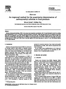
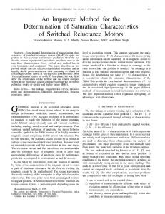
Figure 1. 共a兲 A 32-s raw vertical velocity data record from a 3-C downhole geophone array. 共b兲 Amplitude spectrum of 共a兲 after summing over all traces. 共c兲 Panel 共a兲 after 关75,300兴 Hz band-pass filtering.
FIELD DATA EXAMPLE 5
2
4
3
1
Geophone index
a) 6 4 2 0
5
10
15
20
25
30
5
10
15
20
25
30
5
10
15
20
25
30
Geophone index
b) 6 4 2 0
c) Geophone index
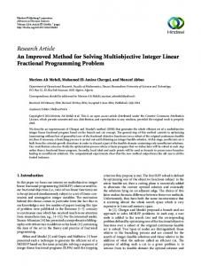
A microseismic survey was performed during the hydraulic fracturing stimulation of a carbonate reservoir in Oklahoma. An eight-level 3-C geophone array was deployed in the monitoring well at a depth from 1385 m 共4545 ft兲 to 1492 m 共4895 ft兲, where we refer to the shallowest as level 1 and the deepest as level 8. The treatment well is approximately 440 m 共1450 ft兲 away from the monitoring well. The perforation was conducted at a depth of 1530 m 共5030 ft兲. Figure 1a shows a segment of the continuous microseismic record. Unfortunately, level 8 failed to work, so only waveforms from seven levels are available. Figure 1b shows that the most energetic part of lowfrequency noise is concentrated mainly below 75 Hz. Additional signal spectral analysis demonstrates that most signal energy is below 300 Hz. Therefore, a band-pass filter of 关75,300兴 Hz was applied to the raw data to get an enhanced signal as shown in Figure 1c. Figure 2 shows the three components 共Z,X,Y兲 of the band-pass filtered data. The band-pass filtered data in Figure 2 show several microseismic events. The standard STA/ LTA event detection algorithm detects the three largest events, which are noted as events 1, 2, and 3 with S-wave arrivals on level 1 at approximately 19.3, 8.3, and 28.0 s, respectively. Another two smaller events 共events 4 and 5兲 around 13.5 and
6 4 2 0
Recording time (s)
Figure 2. 关75,300兴 Hz band-pass filtered velocity data: 共a兲 Z component 共same as Figure 1c兲, 共b兲 X component, 共c兲 Y component. Events 1, 2, and 3 are detected by the STA/LTA detector, with event 1 selected as the master event for the correlation detector. Events 4 and 5, although visible, are hard to detect by the single-geophone STA/LTA detector.
Downloaded 06 Jan 2011 to 18.7.29.240. Redistribution subject to SEG license or copyright; see Terms of Use at http://segdl.org/
A50
Song et al.
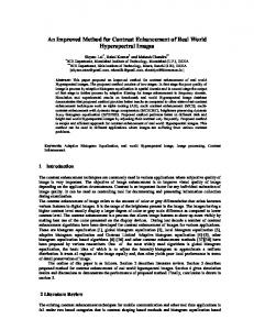
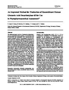
culated SNRs for events 1–5 on the band-pass filtered data are 15.3, 12.4, 11.7, 6.5, and 6.1 dB, respectively. The largest event around 19.3 s is selected as the master event. Figure 3 shows the vertical component 共the Z component兲 crosscorJ N1 3 relation template in which P- and S-wave arrivals are included. We j,k 关s⌬t 共i兲兴2 N1 apply three forms of correlation detector to the 3-C data in Figure k⳱1 j⳱1 i⳱1 2. Figure 4b gives the one-geophone, 1-C correlation result 共level 1, SNR共dB兲 ⳱ 10 log10 , 共10兲 the vertical component兲, whereas Figure 4c and d gives the array3 J N2 stacked correlation traces using only the vertical component and all j,k 2 关n⌬t 共i兲兴 N2 three components, respectively. Compared with the band-pass filk⳱1 j⳱1 i⳱1 tered data in Figure 4a, the one-geophone, one-component correlaj,k j,k where s⌬t 共i兲 and n⌬t 共i兲 denote the kth component data of the event tion detector does not increase the SNR, which indicates the exisand noise segment recorded at the jth receiver, with N1 and N2 being tence of some correlated noise. However, Figure 4c gives better microseismic signal and noise window length, respectively. The calSNRs for two weak events 4 and 5 by stacking the vertical component correlation traces across all seven geophones. The noise correS P lation level has decreased from 0.2 in Figure 4b to 0.05 in Figure 4c after cross-geophone stacking. The correlation level for the weakest 7 event 5 in Figure 4c is 0.45. This means that, by stacking the onecomponent correlation traces, the SNR for the weakest event 5 has 6 increased from 6.1 dB in Figure 4a to 19.0 dB in Figure 4c. Figure 4d represents the array-stacked correlation traces across all three 5 components. The noise correlation level further decreases to 0.03. The SNR for the weakest event 5 increases to 22.5 dB in Figure 4d. 4 This additional 3.5-dB SNR gain over Figure 4c comes from match3 ing in polarization structure by using all three components. Even for the master event 共i.e., the strongest event兲, the SNR on the 3-C array2 stacked correlation detector has been boosted from the original 15.3 dB in Figure 4a to 30.4 dB in Figure 4d. Two weak events 4 and 1 5 are easy to identify in Figure 4d. 19.1 19.15 19.2 19.25 19.3 19.35 For comparison, we also apply the STA/LTA detector to the arrayRecording time (s) stacked 3-C data. Before stacking, a moveout correction is used to Figure 3. Master event waveform as the crosscorrelation template align the waveforms from different geophones. 共vertical component of event 1 as shown in Figure 2a兲. Here the moveout is estimated by crosscorrelating the master event waveform segments between 5 2 1 3 4 geophone pairs. Figure 4e gives the sum of three a) 1 single-component STA/LTA ratios of the stacked 0 band-pass filtered data after the moveout correc–1 tion. The STA and LTA window lengths are se5 0 10 15 20 25 30 lected to be 3 and 15 times the dominant period b) 1 共16 and 80 ms兲, respectively. Although events 1–4 clearly stand out in Figure 4e, event 5 is hard 0 to detect under a reasonable false alarm rate. The –1 5 0 10 15 20 25 30 SNR of the weakest event 5 increases from c) 6.1 to 14.6 dB. This 8.5-dB SNR gain, resulted 1 from moveout corrected array stacking, is smaller 0 than the 16.4-dB gain in the 3-C array-stacked –1 correlation detector. Moreover, a spurious event 5 0 10 15 20 25 30 around 14.8 s 共labeled with an asterisk in Figure d) 1 4e兲 is actually caused by the large noise recorded 0 mainly by geophones 4 and 3 共Figure 2兲, which is –1 not seen in the correlation detector 共Figure 4d兲. 5 0 10 15 20 25 30 This demonstrates the utility of the array-stacked e) 300 correlation detector over the array-stacked STA/ 200 LTA detector. The 3-C array-based correlation 100 detector can effectively enhance the SNR of 5 0 10 15 20 25 30 small microseismic events and therefore is suitTime (s) able to detect small-magnitude events with waveFigure 4. 共a兲 关75,300兴 Hz band-pass filtered vertical velocity data from geophone 1. 共b兲 forms similar to a master event. In practice, we One-component, one-geophone correlation detector output. 共c兲 One-component, arraycan use the STA/LTA detector to identify several stacked correlation detector output. 共d兲 Three-component, array-stacked correlation detector output. 共e兲 Three-component, array-stacked STA/LTA detector output. 2.3 s are noticeable but are hard to detect by the single-geophone STA/LTA detector. To calculate the SNR of these five events, we define
兺兺兺
兺兺兺
冎冒 冎冒
Normalized amplitude STA/LTA Correlation coefficient Correlation coefficient Correlation coefficient
Geophone index
再 再
Downloaded 06 Jan 2011 to 18.7.29.240. Redistribution subject to SEG license or copyright; see Terms of Use at http://segdl.org/
Microseismic event detection & phase picking
a) × 10–6
b)
× 10–6
4
2 2 0 0 –2 –2
c)
19.16 19.18 19.2 19.22 19.24 19.26 19.28
1.0
e)
0.5
19.16 19.18 19.2 19.22 19.24 19.26 19.28
1.0
0.0
f)
19.16 19.18 19.2 19.22 19.24 19.26 19.28
1.0
0.5
0.0
19.16 19.18 19.2 19.22 19.24 19.26 19.28
1.0
0.5
0.0
d)
0.5
19.16 19.18 19.2 19.22 19.24 19.26 19.28
0.0
19.16 19.18 19.2 19.22 19.24 19.26 19.28
Time (s)
Time (s)
Manual picks
Transformed spectrogram picks
STA/LTA picks
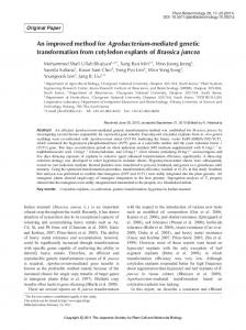
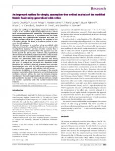
Figure 5. Comparison of manual picks 共solid line兲, transformed spectrogram picks 共dashed line兲, and STA/LTA picks 共dashed-dotted line兲. 共a兲 P-wave arrival picks on bandpass filtered X component data from geophone 1 for event 1 共the master event兲. 共b兲 S-wave arrival picks on band-pass filtered Z component data from geophone 1 for event 1. 共c兲 Characteristic function, as specified in equation 9, ¯S共关75,300兴,t兲 for the X component data, in which P-wave arrival is identified as the first major peak. 共d兲 ¯S共关75,300兴,t兲 for the Z component data, where S-wave arrival is identified as the second major peak. 共e兲 STA/LTA function for X component data. 共f兲 STA/LTA function for Z component data.
b)
a) × 10–7
× 10–7
1.0
5
0.5
0
0.0 –0.5
–5
–1.0
c)
2.22
2.24
2.26
2.28
2.3
2.32
1.0
e)
2.24
2.26
2.28
2.3
2.32
2.22
2.24
2.26
2.28
2.3
2.32
2.22
2.24
2.26
2.28
2.3
2.32
0.5
2.22
2.24
2.26
2.28
2.3
2.32
1.0
0.0
f)
1.0
0.5
0.0
2.22
1.0
0.5
0.0
d)
0.5
2.22
2.24
2.26
2.28
2.3
2.32
0.0
Time (s) Manual picks
A51
large events, which can then be used as master events to detect their nearby weak events. For each detected event, we use the multitaperbased transformed spectrogram approach as described in equations 7–9 to identify the P- and S-wave arrivals and compare them with standard STA/LTA picks 共Earle and Shearer, 1994兲. We calculate the characteristic function ¯S共关 f 1,f 2兴,t兲 to pick the P- and S-wave arrivals on each 3-C geophone for each detected event. Here 关 f 1,f 2兴 is set as the microseismic signal frequency range, 关75,300兴 Hz. The method is applied to all three components to get the optimal P- and S-wave arrival picks. The P- and S-wave arrivals can be picked separately from the component that has the best P- and S-wave SNRs or together from the sum of ¯S共关 f 1,f 2兴,t兲 over all three components. In our study, both methods give similar P- and S-wave picks. For the level 1 geophone, Figure 5 compares the manual picks 共solid line兲, transformed spectrogram picks 共dashed line兲, and STA/LTA picks 共dashed-dotted line兲 for the master event. P- and S-waves separately have the highest SNR on the horizontal and vertical component. Thus, the P-wave arrival is determined from the horizontal component, whereas the S-wave arrival is obtained from the vertical component. For this large event, the arrivals given by both methods are close to the manual picks, signifying that we can use the STA/LTA detector to identify master events and determine tM. The arrivals identified by the peaks on ¯S共关75,300兴,t兲 are close to the onset of phase arrivals, whereas the STA/LTA picks tend to give the peak arrival times. For the weakest event, as shown in Figure 6, the STA/LTA picks have little agreement with manual picks because of the high noise level, whereas the transformed spectrogram picks are consistent with manual picks. This illustrates that the transformed spectrogram facilitates picking of weak phase arrivals. The noise level has less influence on the characteristic function because of the differentiation term in equation 7. The shape of the characteristic function depends on the signal energy distribution in the time-frequency domain, and the window length L. The choice of L depends on the balance between the sharpness of the P- and S-peaks 共i.e., the resolution of arrival picks兲 and the occurrence of spurious peaks. From our experience, three to four times the dominant period is a good value.
Time (s) STA/LTA picks
Transformed spectrogram picks
Figure 6. Comparison of manual picks 共solid line兲, transformed spectrogram picks 共dashed line兲, and STA/LTA picks 共dashed-dotted line兲. 共a兲 P-wave arrival picks on bandpass filtered X component data from geophone 1 for event 5 共the weakest event兲. 共b兲 S-wave arrival picks on band-pass filtered Z component data from geophone 1 for event 5. 共c兲 Characteristic function, as specified in equation 9, ¯S共关75,300兴,t兲 for the X component data, where P-wave arrival is identified as the first major peak. 共d兲 ¯S共关75,300兴,t兲 for the Z component data in which S-wave arrival is identified as the second major peak. 共e兲 STA/LTA function for X component data. 共f兲 STA/LTA function for Z component data.
CONCLUSIONS In this paper, we have proposed a systematic approach for hydrofracture event detection and phase picking. By field test, we have demonstrated that once the standard STA/LTA detector detects a large event, it can be used as the master
Downloaded 06 Jan 2011 to 18.7.29.240. Redistribution subject to SEG license or copyright; see Terms of Use at http://segdl.org/
A52
Song et al.
event. A 3-C array-stacked correlation detector using this master event template can effectively increase the detectability of nearby small-magnitude events. Unlike conventional array stacking of the waveform data from one single event, the array stacking of correlation traces between two close events suffers no coherence loss and requires no knowledge of the velocity model. Under the same false alarm rate, the array-stacked correlation detector gives better results than the array-stacked STA/LTA detector because the correlation detector uses full waveform information. The 3-C, array-stacked processing is superior to a single-component, single-geophone correlation detector. The processing gain increases with the increased number of geophones. The limitation of the correlation detector is that it is only capable of detecting the events that are within one dominant wavelength from the master event. However, this limitation could be alleviated by updating the master event. For phase picking, we have applied the transformed spectrogram approach to identify the weak arrivals. The P- and S-wave arrivals are picked from the component that has the highest SNR for P- and S-wave vector. The transformed spectrogram captures two features of a phase arrival in the time-frequency domain, high energy and high rate of energy increase; therefore, it improves phase picking. Detection and phase identification of small-magnitude microseismic events have potential for not only hydrofracture monitoring but also reservoir surveillance.
ACKNOWLEDGMENTS We thank the Halliburton Energy Services Company Houston office for providing the data and for funding this research. We greatly appreciate valuable comments from Leo Eisner, three anonymous reviewers, and the editor. We are grateful to Norman R. Warpinski from Halliburton Energy Services Company for his helpful suggestions. We thank Halliburton Energy Services Company for permission to publish this work.
REFERENCES Arrowsmith, S. J., and L. Eisner, 2006, A technique for identifying microseismic multiplets and application to the Valhall field, North Sea: Geophysics, 71, no. 2, V31–V40, doi: 10.1190/1.2187804 De Meersman, K., J.-M. Kendall, and M. van der Baan, 2009, The 1998 Valhall microseismic data set: an integrated study of relocated sources, seismic multiplets, and S-wave splitting: Geophysics, 74, no. 5, B183–B195, doi: 10.1190/1.3205028 Earle, P. S., and P. M. Shearer, 1994, Characterization of global seismograms using an automatic-picking algorithm: Bulletin of the Seismological Soci-
ety of America, 84, 366–376. Eisner, L., D. Abbott, W. B. Barker, J. Lakings, and M. P. Thornton, 2008, Noise suppression for detection and location of microseismic events using a matched filter: 78th Annual International Meeting, SEG, Expanded Abstracts, 1431–1435. Eisner, L., P. M. Duncan, W. M. Heigl, and W. R. Keller, 2009a, Uncertainties in passive seismic monitoring: The Leading Edge, 28, 648–655, doi: 10.1190/1.3148403 Eisner, L., T. Fischer, and J. H. L. Calvez, 2006, Detection of repeated hydraulic fracturing 共out-of-zone growth兲 by microseismic monitoring: The Leading Edge, 25, 548–554, doi: 10.1190/1.2202655 Eisner, L., T. Fischer, and J. T. Rutledge, 2009b, Determination of S-wave slowness from a linear array of borehole receivers: Geophysical Journal International, 176, no. 1, 31–39, doi: 10.1111/j.1365-246X.2008.03939.x Gibbons, S. J., and F. Ringdal, 2006, The detection of low magnitude seismic events using array-based waveform correlation: Geophysical Journal International, 165, no. 1, 149–166, doi: 10.1111/j.1365-246X.2006.02865.x Gibbons, S. J., F. Ringdal, and T. Kvaerna, 2008, Detection and characterization of seismic phases using continuous spectral estimation on incoherent and partially coherent arrays: Geophysical Journal International, 172, no. 1, 405–421, doi: 10.1111/j.1365-246X.2007.03650.x Kao, H., and S.-J. Shan, 2004, The source-scanning algorithm: Mapping the distribution of seismic sources in time and space: Geophysical Journal International, 157, no. 2, 589–594, doi: 10.1111/j.1365-246X.2004.02276.x. Kristiansen, T., O. Barkved, and P. Patillo, 2000, Use of passive seismic monitoring in well and casing design in the compacting and subsiding Valhall field, North Sea: SPE Paper 65134. Maxwell, S., and T. Urbancic, 2002, Real-time 4D reservoir characterization using passive seismic data: SPE Paper 77361. Michelet, S., and M. N. Toksöz, 2007, Fracture mapping in the Soultz-sousForêts geothermal field using microearthquake locations: Journal of Geophysical Research, 112, B7, B07315, doi: 10.1029/2006JB004442. Pavlis, G., 1992, Appraising relative earthquake location errors: Bulletin of the Seismological Society of America, 82, 836–859. Phillips, W., J. Rutledge, L. House, and M. C. Fehler, 2002, Induced microearthquake patterns in hydrocarbon and geothermal reservoirs: six case studies: Pure and Applied Geophysics, 159, no. 1, 345–369, doi: 10.1007/ PL00001256. Ronen, J., and J. F. Claerbout, 1985, Surface-consistent residual static estimation by stack-power maximization: Geophysics, 50, 2759–2767, doi: 10.1190/1.1441896. Rowe, C., R. Aster, W. Phillips, R. Jones, B. Borchers, and M. Fehler, 2002, Using automated, high-precision repicking to improve delineation of microseismic structures at the Soultz geothermal reservoir: Pure and Applied Geophysics, 159, no. 1, 563–596, doi: 10.1007/PL00001265. Stein, S., and M. Wysession, 2002, An introduction to seismology, earthquakes and earth structure: Wiley-Blackwell. Thomson, D. J., 1982, Spectrum estimation and harmonic analysis: Proceedings of the IEEE, 70, no. 9, 1055–1096, doi: 10.1109/PROC.1982.12433. Walker, R. N. Jr., 1997, Cotton Valley hydraulic fracture imaging project: SPE Paper 38577. Willis, M. E., D. R. Burns, K. M. Willis, N. J. House, and J. Shemeta, 2008, Hydraulic fracture quality from time lapse VSP and microseismic data: 78th Annual International Meeting, SEG, Expanded Abstracts, 1565–1569. Willis, M. E., K. M. Willis, D. R. Burns, J. Shemeta, and N. J. House, 2009, Fracture quality images from 4D VSP and microseismic data at Jonah Field, WY: 79th Annual International Meeting, SEG, Expanded Abstracts, 4110–4114.
Downloaded 06 Jan 2011 to 18.7.29.240. Redistribution subject to SEG license or copyright; see Terms of Use at http://segdl.org/