An Improved Moving-Window Method for Shot Boundary Detection Hao Xie, Ruofeng Tong College of Computer Science and Technology Zhejiang University Hangzhou, China
[email protected],
[email protected]
Abstract—Shot Boundary Detection is an important phase in the process of video retrieval, thus an automatic way to do this work is imperative. In this paper, we present an improved movingwindow approach which can tackle this problem effectively. In our method, an existing concept of moving window is adopted. Then the Manhattan distance of histograms in RGB color space and the Laplace transform of each frame are calculated as the measurement of similarity. And finally each frame is examined through several classifiers to determine whether it is a component of a transition. The innovation of this paper is to apply Laplace transform as a supplementation of current features, and to propose a flexible video-dependent threshold, which leads to a higher precision. Experiments show that our approach can generate preferable results in most cases compared with two previous methods. Keywords: video; shot boundary detection; histogram; Laplace transform; and moving window
I.
INTRODUCTION
Nowadays, the information technology is developing swiftly, one probable result of which is that the everyday volume of video resources has become larger, and the resources themselves are also out of order. In order to make full use of the mass of video resources, we need to classify them according to their contents. A previous, also important, work during the process of classification is to break a video into pieces of sub-videos, principally containing a unique shot or scene. And the key point is to identify the temporal position of transition between two adjacent shots, which is called Shot Boundary Detection (SBD) or Temporal Video Segmentation (TVS). Generally speaking, a transition between two adjacent shots consists of three parts: the Beginning Frame (BF, the last frame of the former shot), the Ending Frame (EF, the first frame of the latter shot) and the Transitional Frames (TF, the frames between BF and EF). There are two types of transitions: abrupt transition (AT, also called “cut”, fig. 2 is an example) and gradual transition (GT, see fig. 3). And the only difference between them is: GT has some TF(s), while AT does not. Our aim is to find out all BFs and EFs in a video to split the original video into pieces of sub-videos. In detail, BFs and EFs belong to former and latter shots, respectively, while the TF, if exists, belongs to neither.
Methods for AT detection could achieve a success percentage of more than 90% for most types of videos. The simplest way to detect an AT is pixel-wised method [6~8], but the results are not quite acceptable, because the pixel difference of two frames can only carry little useful information and usually causes confusions. A reasonable improvement is to use color histograms of images [1], [9], [10] as the feature, which is also an effective way for AT detection. As an enhancement of current approaches, another novel thought [11~13] integrates several simple methods, draw their advantages and also have a good result. On the contrary, approaches on GT detection are not as successful as to those on ATs. Due to the complexity and diversification of GTs, most methods [14~19] only focus on limited types of effects, e.g. fades (in and out), dissolves and wipes. Some methods are based on edge detection [15], others use statistical approach [16], [17], [20], [21], and still others employ the histograms [2]. And all of them can produce a relatively pleasant result. Nevertheless, some complicated GTs, such as geometric transitions, are still a challenge. Those methods above are mostly aiming at single type of transition; however, unified approaches [6], [22~24] for both ATs and GTs also play an important role. Bescós et al. [23] maps the distance space into a new space and reaches a better result. Yuan et al. [25] gives a formal comprehensive study and also propose a graph-based framework. Another new thought [26] is based on clustering and optimization. In this paper, we propose an effective approach which is based on a moving-window framework to detect ATs and some simple GTs. Firstly, we adopt an existing concept of moving window [1], [2]. Secondly, we use 256-bin histograms in RGB color space and Laplace transform of frames as the measurement of similarity. And finally, through several classifiers, a frame is examined to determine whether it is a BF/EF. The innovation of this paper is the usage of Laplace transforms as a supplementation of current feature, and a flexible threshold depending on the video itself, instead of a fixed one. This method can generate a better result than others from most ATs and some simple GTs, but in some complicated cases, especially the irregular geometric transitions between two blocks of news, it seems to be somewhat powerless. We organize this paper as follows: In section 2, we review and analyze the existing moving-window framework. In
This project is supported by National High-Tech Research and Development Program (No. 2009AA01Z330) of China
978-1-4244-4994-1/09/$25.00 ©2009 IEEE
section 3, we expound the process of our method in detail. As a supplementation of the previous section, we explain the choice of similarities and the calculation of distances in section 4. And in section 5, we describe our experiments in detail, show some results of our experiments compared with the other two methods, and list some additional remarks. II.
ANALYSIS OF PREVIOUS WORKS
In this section, we briefly review and analyze two framewindow methods [1], [2]. The first algorithm [1] makes good results for ATs, whose process is shown below. For each current frame in the video, except some frames in the beginning and ending of the video: •
Define a fixed-size moving window, consisting of equal-sized pre- and post-frames preceding and following the current frame in the middle, which is not included in the window, respectively. (see fig. 2)
•
Sort all the frames in the window, according to their distances to current frame, which we will explain in section 4. The frame with smaller distance has the higher rank.
•
Calculate the pre-frame number, the number of preframes in the top-half rank, and a transition is detected if the curve of pre-frame number goes through an upper threshold and a lower threshold in turn within a small number of consecutive frames, say 4 or 6 frames.
As a supplement and improvement of the first method, the second method [2] is applied for GTs. Instead of sorting the frames and calculating the pre-frame number, this approach defines for each current frame a pre-post ratio, which is the ratio of the pre- and post-value of average-histogram distance. This ratio reaches a local minimum at a BF, and a local maximum at the corresponding EF. And a transition is recognized when the curve of pre-post ratio goes from the local minimum, up through two moving thresholds and finally to the local maximum. Both approaches have good results, especially the one for ATs. However, there still are some flaws. The first and also important aspect is that the choice of features. Here, both methods simply take the histograms in HSV color space as the feature. This might not adapt to all situations, e.g. two frames with similar color histograms belong to two different shots respectively. In this case, a transition would be missed definitely. Similarly, an error might also occur when two adjacent frames, belonging to one shot, have drastic color disparity, e.g. in the scene under the neon lights in a bar, the colors of frames changes frequently, but the edge information does not. Therefore, it is necessary to add other features to similarity calculation. Another aspect is the threshold, which can be classified into global and local, also called static threshold and dynamic one. A global threshold means all data use the same fixed threshold, which is easier to handle but lack of flexibility; while a local one refers to a variable threshold suitable for different data. In this case, the method [1] for ATs uses static threshold for simplicity, and generates a good result from certain videos. As
an improvement of the first method, the second one [2] utilizes two dynamic thresholds to detect GTs. III.
SHOT BOUNDARY DETECTION USING THE IMPROVED MOVING-WINDOW METHOD
In this section, we will explain our method in detail. For each current frame in the video: first, we define a moving frame window, as the first method [1] does in step 1, and refer to the number of pre- or post- frames as half window size (HWS, see fig. 2); second, we calculate the distance d k
f c and each frame f c + k in the window, k = ±1," , ± HWS , which will be discussed in
between the current frame
section 4; and finally, according to some classifiers, we determine whether the current frame is a BF or EF. Here, we mainly discuss the last step. Observing the features of transitions, we find that at BFs, distances from current frame to pre-frames (called pre-dist) are smaller than those to post-frames (called post-dist), and vice versa at EFs. Thus, for convenience here, we mainly focus on the way to identify BFs. Based on the above observation, an intuition is that, if the maximum of the pre-dist d − max is smaller than the minimum of the post-dist d + min , a BF is found. In short, the first classifier can be represented as:
C1 = { f c d − max ≤ d + min }
(1)
Apart from the maximum and minimum value of distances, the average value is also an important factor for SBD, which can utilize the information in the window more abundantly. As an enhancement of the first classifier, we require that the average value of post-dist is more than twice of the corresponding value of pre-dist:
C2 = ® f c ¯
HWS
¦d k =1
+k
HWS ½ ≥ 2 ¦ d−k ¾ k =1 ¿
(2)
In some low quality videos, a noise frame might exist somewhere, which divides a continuous shot into two parts, and thus an error in SBD appears when the noise is the current frame. In order to avoid this type of errors in a shot, we require the distance between two neighbor frames of the current frame, which is the distance between the last pre-frame and the first post-frame, is reasonably large. Here we require this distance to be larger than one quarter of the maximum of post-dist, which is the third classifier:
d ½ C3 = ® f c dist ( f c −1 , f c +1 ) ≥ + max ¾ 4 ¿ ¯
(3)
All of the above classifiers only use the ratio relationship of the distance values, which might not cover all aspects. Suppose
we have a shot containing many similar continuous frames, one of which satisfies all conditions above. Apparently, it is mistaken for a BF by classifiers above. The reason of this is: although the ratio of distances for this frame is large enough, the absolute distance is too small, so that the frame should not be considered as a BF. Thus it is also necessary to monitor absolute values. For this purpose, we require the absolute value of distances to be large enough to avoid the situation above. A simple way is to set a static threshold, but it can only adapt to a few situations. Therefore, we employ variable thresholds to solve this problem. In particular, we keep a historical record of minimum (or maximum) pre-dist (or post-dist) series, which are not generated from BFs/EFs, and compute the sum of their average and deviation values as the dynamic threshold, denoted by thd . Only the frame whose minimum (or maximum) predist is larger than the threshold should be considered as a BF/EF candidate. Fig. 4 shows the relationship between minimum pre-dist and the dynamic threshold.
histogram respectively. As for the second type, we first calculate the Laplace transform for each color band of a frame, and then sum the absolute value of subtractions of pairs of corresponding pixel values, as shown in (6), where width and height means the size of a frame, r’, g’, b’ denote the pixel value of 3 channels of a frame after Laplace transform. In our method, a transition is detected if either of these two distances satisfies the classifiers mentioned in section 3.
dist ( fi , f j ) = ¦ k =1 ri ( k ) − rj ( k ) depth
+ ¦ k =1 gi ( k ) − g j ( k ) depth
+ ¦ k =1 bi ( k ) − b j ( k ) depth
dist ′ ( f i , f j ) = ¦ m=1
width
C4 = { f c d − min > thd } Finally, a frame is considered as a BF, if it passes through classifiers (1), (2), (3) and (4) in turn, and the detection of EF is similar. Once BFs and EFs are identified respectively, a tiny problem comes out: the BFs and EFs might not meet the oneto-one relationship, e.g. a BF is detected, but its corresponding EF is not. This makes it difficult to save the result sub-videos according to the BFs and EFs. In order to solve this problem, we simply insert a corresponding EF or BF to match the single BF or EF artificially, so that the new pair can represent an abrupt transition. Although this remedy results in some errors, it decreases misses effectively. IV.
DISTANCE CALCULATION
In this section, we explain how to calculate the distance between two frames. For images, there are many types of features, and also many types of way to measure them. In space domain, the feature of images includes pixel-wised values (intensity, such as RGB, HSV, YUV, CIELAB, CIELUV [4], etc), and gradient of them; while in frequency domain, the feature consists of DCT, FFT, DWT and so on. All of the above features have their own advantages. The intensity represents the whole color information of an image, while the gradient stands for the edge features of an image, which is an important supplement of the intensity and can be used to represent motion information. As for the criteria of features, we can choose the Euclidean distance or Manhattan distance, which is easier to calculate, of the pixel-wised values or histograms. In this paper, we use the Manhattan distance of 8-bit color histograms in RGB color space and the Laplace transform between two frames. Specifically, we first calculate the RGB histograms of two frames, and then sum the absolute values of subtractions of pairs of corresponding bins in two histograms from two frames, thus we have the first type of distances, as shown in (5), where depth means the number of bins in one histogram, r, g, b represent bin values of 3 color bands in a
(5)
¦ +¦ ¦ +¦ ¦
V.
height n =1
width
height
m =1
n =1
width
height
m =1
n =1
ri′( m,n ) − rj′ ( m,n ) gi′ ( m,n ) − g ′j ( m,n ) (6) bi′ ( m,n ) − b′j ( m,n )
EXPERIMENTS AND RESULTS
In this section, we describe our experiment in detail. We first describe the experiments, including the influences caused by thresholds, and then show some results of comparison. To measure the performance of different methods, we adopt the most commonly used way in [3], which is to calculate their recalls (R) and precisions (P), for ATs and GTs respectively, as shown in (7) and (8), where correct means the number of transitions which are correctly detected, miss represent the number of transitions which are NOT recognized, and error denotes the number of frame sequences which are mistaken as transitions.
R=
correct correct + miss
(7)
P=
correct correct + error
(8)
For some resource constrains, the test videos in our experiment are some international news (cctv4.avi and can.avi) and an MTV (liang.avi), as shown in Table I. In order to keep the comparison a fair one, we implement the previous methods ourselves, and test them using the same test videos under the same situations. Thus, the results of previous approaches might have some deviations in relation to their primary implementations, but the rough relationship between these methods is shown correctly. As illustrated in fig. 1, results produced by our approach are mostly better than those
generated by others, except some GT ones, which appear better results by the method for GTs [2]. TABLE I.
shorter than one second, which is supposed to be meaningless for Shot Boundary Detection. VI.
DETAILS OF OUR TEST MATERIALS
Filename
Type
Frames
Abrupt
Gradual
Cctv4.avi
News
44830
9
434
can.avi
News
126063
734
259
liang.avi
MTV
6484
11
81
CONCLUSION
Artificial shot boundary detection used to be a tedious job in the whole process of video management, thus an automatic style is imperative. Fortunately, many algorithms can solve this problem, and most of them generate preferable results for ATs and certain simple GTs. However, for complicated GT detection, an unbridgeable gap still blocks in our way. In this paper, we propose an effective method, which is an improvement of the moving-window method. In our method, we adopt the concept of moving window, add Laplace transform to the framework as an innovation, and propose a dynamic threshold to decrease errors effectively. In our experiments, we implement and compare different methods. As shown in the results, our approach makes a better result, although some complex transitions are still difficult to recognize. Technically, the selection of features has a large space to exploit, and the statistics or stochastic processes can be added to the main framework. We believe these thoughts give a new direction, which is also our possible future work. ACKNOWLEDGMENT
Figure 1. Comparision result of different methods. The “method_AT” and “method_GT” represent two methods mentioned in section 2, and the “our_RGB” denotes our method. “cctv4”, “cna”, and “liang” are our test cases
There might also be small deviations (usually 1 to 5 frames) for GTs between the real results and the standard results counted by us, so it is to be noted here that we set the sensitivity to be 2 frames for ATs and 5 for GTs, which means that the output results are correct, if the deviation between the output results and standard results is less than 2 frames. In addition, no TF appears in an AT by the concept mentioned in section 1, however, many AT-like GTs only have 1 or 2 TFs, thus might cause some confusions. Here we strictly do the detection based on the standard definition of ATs, although this would be different from others. Several factors are responsible for the final result of the current method. The most important one is the choice of distance calculation, which is partially mentioned above. Here, we test our method with several features, including RGB, HSV, and a new color space [5], which is robust to spectral changes in illumination, and the result shows that they almost have the same results. Among these color spaces, the RGB color space is the simplest and most effective one, thus becomes our choice. Apart from distance, the size of half window (HWS) is also an important factor, and its effect is mentioned in [1]. In general, smaller HWS can increase the sensitivity and the errors, while larger HWS can increase the misses. In [1], the author used fixed value of HWS, which is not suitable for all the situations. In this paper, we use a flexible value, depending on the video to be processed and give a preferable result. In order to achieve the best result, we set the value to be half fps of the video. This implies that we cannot detect a video shot
The authors sincerely acknowledge Sheng Zhou at National Defense University of PLA for test videos. The authors also acknowledge the constructive comments and suggestions by the referees. REFERENCES [1]
S. M. M. Tahaghoghi, H. E. Williams, J. A. Thom, and T. Volkmer, “Video Cut Detection using Frame Windows,” ACSC’05. [2] T. Volkmer, S. M. M. Tahaghoghi, and H. E. Williams, “Gradual Transition Detection Using Average Frame Similarity,” IEEE CVPRW’04. [3] J. S. Boreczsky and L. A. Rowe, “Comparison of video shot boundary detection techniques,” in Proc. SPIE, vol. 2670, Jan. 1996, pp. 170–179. [4] Watt. A. H, Fundamentals of Three-Dimensional Computer Graphics, Addison Wesley, Wokingham, UK. 1989. [5] H. Y. Chong, S. J. Gortler, and T. Zickler, “A Perception-based Color Space for Illumination-invariant Image Processing,” SIGGRAGH 2008. [6] B. Yeo and B. Liu, “A unified approach to temporal segmentation of motion JPEG and MPEG compressed video,” in Proc. ACM Multimedia, San Francisco, CA, Nov. 1995, pp. 81–88. [7] K. Otsuji and Y. Tonomura, “Projection detecting filter for video cut detection,” in Proc. ACM Multimedia’93, Anaheim, CA, Aug. 1993, pp. 251–256. [8] A. Dailianas et al., “Comparison of automatic video segmentation algorithms,” in Proc. SPIE Conference on Integration Issues in Large Commercial Delivery Systems, Philadelphia, PA, Oct. 1995. [9] H. Ueda et al., IMPACT: “An interactive natural-motion picture dedicated multimedia authoring system,” in Proc. CHI’91 Conf., New Orleans, LA, April 1991, pp. 343–350. [10] A. Nagasaka and Y. Tanaka, “Automatic video indexing and full-video search for objects appearances,” in Proc. IFIP 2nd Conf. Visual Database Systems, Budapest, Hungary, Sep. 1991, pp. 113–127. [11] H. D. Wactlar et al., “Automated video indexing of very large video libraries,” SMPTE J., pp. 524–529, Aug. 1997.
[12] M. R. Naphade et al., “A high performance shot boundary detection algorithm using multiple cues,” in Proc. ICIP’98, vol. 1, Chicago, IL, Oct. 1998, pp. 884–887. [13] Y. Yusoff, J. Kittler, and W. Christmas, “Combining multiple experts for classifying shot changes in video sequences,” in Proc. IEEE Multimedia Systems’99, vol. 1, Florence, Italy, Jun. 1999, pp. 700–704. [14] B. T. Truong, C. Dorai, and S. Venkatesh, “New enhancements to cut, fade, and dissolve detection processes in video segmentation,” in R. Price, editor, Proceedings of the ACM International Conference on Multimedia 2000, pages 219–227, Los Angeles, CA, USA, 30, October – 4, November, 2000. [15] R. Zabih, J. Miller, and K. Mai, “A feature-based algorithm for detecting and classifying production eects,” Multimedia Systems, vol. 7, no. 2, pp. 119–128, 1999. [16] W. A. C. Fernando, C. N. Canagarajah, and D. R. Bull, “Fade and dissolve detection in uncompressed and compressed video sequences,” in Proc. IEEE International Conference on Image Processing (ICIP ’99), vol. 3, pp. 299–303, Kobe, Japan, October 1999. [17] R. Lienhart, “Comparison of automatic shout boundary detection algorithms,” in SPIE Image and Video Processing VII, vol. 3656, pp. 290–301, San Jose, Calif, USA, January 1999. [18] H. Zhang, A. Kankanhalli, and S. Smoliar, “Automatic partitioning of full-motion video,” Multimedia Systems, vol. 1, no. 1, pp. 10–28, 1993. [19] B. L. Yeo, “Efficient processing of compressed images and video,”
Pre-frames
[20]
[21]
[22]
[23]
[24]
[25]
[26]
Current Frame
Ph.D. thesis, Department of Electrical Engineering, Princeton University, Princeton, NJ, USA, January 1996. C. W. Ngo, T. C. Pong, and R. T. Chin, “Detection of gradual transitions through temporal slice analysis,” in Proc. IEEE Computer Society Conference on Computer Vision and Pattern Recognition (CVPR ’99), vol. 1, pp. 36–41, Fort Collins, Colo, USA, June 1999. M. G. Chung, J. Lee, H. Kim, S. M.-H. Song, and W. M. Kim, “Automatic video segmentation based on spatio-temporal features,” Korea Telecom Journal, vol. 4, no. 1, pp. 4–14, 1999. P. Bouthemy, M. Gelgon, and F. Ganansia, “A unified approach to shot change detection and camera motion characterization,” IEEE Trans. Circuits Syst. Video Technol., vol. 9, no. 7, pp. 1030–1044, Oct. 1999. J. Bescós, G. Cisneros, J. M. Martínez, J. M. Menendez, and J. Cabrera, “A unified model for techniques on video shot transition detection,” IEEE Trans. Multimedia, vol. 7, no. 2, pp. 293–307, Apr. 2005. J. Yuan, J. Li, F. Lin, and B. Zhang, “A unified shot boundary detection framework based on graph partition model,” in Proc. ACM Multimedia 2005, Nov. 2005, pp. 539–542. J. Yuan, H. Wang, L. Xiao, W. Zheng, J. Li, F. Lin, and B. Zhang, “A formal study of shot boundary detection,” IEEE Trans. Circ. and Sys, for Vid. Tech., 17(2):168–186, 2007. N. Ozay, M. Sznaier, O. I. Camps, “Sequential Sparsification for Change Detection,” CVPR 2008.
Post-frames
Moving Window (excluding the current frame, HWS = 3)
Figure 2. Illustration of a moving window consisting of two sequence of continous frames (pre-frames and post-frames), not including the current frame. In this moving window, there is an AT: the current frame is a BF and should be recognized. The HWS is explained in section 3
Figure 3. An example of complicated geometric GT
Figure 4. Plot of minimum distances between current frame and pre-frames over a 300-frame interval of the video “liang.avi”, the dynamic threshold is calculated from a history of the corresponding distances with regard to non-transition frames