An improved multimodal method for sound propagation in nonuniform lined ducts WenPing Bi,a兲 Vincent Pagneux, Denis Lafarge, and Yves Aurégan Laboratoire d’Acoustique de I’Université du Maine, UMR CNRS 6613, Av. O Messiaen, 72085 Le Mans Cedex 9, France
共Received 6 December 2006; revised 6 April 2007; accepted 13 April 2007兲 An efficient method is proposed for modeling time harmonic acoustic propagation in a nonuniform lined duct without flow. The lining impedance is axially segmented uniform, but varies circumferentially. The sound pressure is expanded in term of rigid duct modes and an additional function that carries the information about the impedance boundary. The rigid duct modes and the additional function are known a priori so that calculations of the true liner modes, which are difficult, are avoided. By matching the pressure and axial velocity at the interface between different uniform segments, scattering matrices are obtained for each individual segment; these are then combined to construct a global scattering matrix for multiple segments. The present method is an improvement of the multimodal propagation method, developed in a previous paper 关Bi et al., J. Sound Vib. 289, 1091–1111 共2006兲兴. The radial rate of convergence is improved from O共n−2兲, where n is the radial mode indices, to O共n−4兲. It is numerically shown that using the present method, acoustic propagation in the nonuniform lined intake of an aeroengine can be calculated by a personal computer for dimensionless frequency K up to 80, approaching the third blade passing frequency of turbofan noise. © 2007 Acoustical Society of America. 关DOI: 10.1121/1.2736785兴 PACS number共s兲: 43.50.Gf, 43.20.Mv, 43.20.Fn, 43.20.Hq 关LLT兴
I. INTRODUCTION
Numerous methods have been proposed to study sound propagation in ducts with locally reactive liners which are mathematically represented by an impedance boundary condition. In the presence of circumferential variations of the lining impedance 共e.g., hard walled splices in lined intakes of aeroengine兲, the problem to solve is fully three dimensional. When dimensionless frequency K is high, where K = kR, k = 2 f / c, f is frequency, c is sound velocity in air, and R is the radius of duct, it turns out to be challenging to model it efficiently. The finite element method 共FEM兲,1,2 perturbation method,3 and point matching method4 have all been proposed to model the sound propagation in nonuniform lined ducts. An equivalent surface source method5 and kinetic theory6 were also employed to analyze the acoustic field in ducts lined with complicated distributions of impedance. The hybrid analytical/numerical methods are always interesting, in which analysis is taken as far as possible. One of the hybrid analytical/numerical methods may be the mode matching method. Modes are first calculated in segmented uniform lined ducts and then matched between different uniform segments. When the lining impedance is circumferentially nonuniform, the sound pressure and particle velocity field cannot be separated in the r − plane, the dispersion relation in one segment cannot be written explicitly, and it is not possible to use classical root finding routines to determine the eigenmodes. Watson7 used a hard walled duct mode expansion series to numerically evaluate the eigenmodes
a兲
Electronic mail:
[email protected]
280
J. Acoust. Soc. Am. 122 共1兲, July 2007
Pages: 280–290
without flow. The Galerkin method was employed to force the series to satisfy the true boundary condition in the lined segment. The complex modal output amplitudes for a specified source distribution were then obtained by applying a mode matching technique at the discontinuity between rigid and lined segments. Fuller8,9 expanded the circumferential admittance function as a Fourier series and the eigenmodes over the separable components adapted to the cylindrical coordinates. He obtained the eigenequation set without flow to be solved. The axial wave numbers in the lined segment were then calculated by solving this set of equations using the method of Muller. Campos et al.10 studied acoustic modes in a cylindrical duct with an arbitrary wall impedance distribution with flow. When the wall impedance varies along the circumference, they calculate the acoustic modes in a similar way as Fuller.8 Wright11 used FEM to calculate the modes and then analytically matched them to the rigid duct modes. Wright et al.12 also extended it to include uniform flow. Astley et al.13 proposed a finite element mode matching method for propagation in lined ducts with flow in which the modes are calculated by FEM and numerically matched by a modified Galerkin method. In Ref. 14, we proposed a multimodal propagation method 共MPM兲 to study sound propagation in a nonuniform lined duct without flow. The sound pressure is expressed as a double series of the rigid duct modes which are known a priori. By matching the pressure and axial velocity at the interface between different segments, scattering matrices are obtained for each individual segment and then combined to construct a global scattering matrix for multiple segments. Different kinds of sources can be easily integrated without recalculating the scattering matrix. The full threedimensional 共3D兲 problem is reduced to a two-dimensional
0001-4966/2007/122共1兲/280/11/$23.00
© 2007 Acoustical Society of America
FIG. 1. Configuration of one axial segment nonuniform lined duct.
one which is better suited for the study of acoustic propagation in the lined intake of an aeroengine. The boundary condition is satisfied in the integral sense. Unlike the methods cited earlier, calculations of the eigenmodes of nonuniform lined ducts, which are very difficult, are avoided. This method is also extended to include uniform flow.15 Because the individual rigid duct mode does not satisfy the impedance boundary condition, the radial convergence rate is only O共n−2兲, where n is the radial mode indices. In this paper, we improve the MPM14 by accelerating the radial convergence rate. The sound pressure is expressed as a double series of the rigid duct modes and an additional function which carries the information of the impedance boundary. This is motivated by Ref. 17 which studies water waves over variable bathymetry regions, and Refs. 18 and 19 which study sound propagation in rigid waveguides with varying cross section. It is shown that the radial convergence rate of the double infinite series is improved from O共n−2兲 to O共n−4兲. This improvement can be extended to include uniform flow.16 The paper is organized as follows. In Sec. II, the derivation of equations are presented for circumferentially uniform and nonuniform boundary conditions, respectively. The convergence properties are then shown analytically and numerically in Sec. III. Finally, in Sec. IV, we present some numerical examples to show the robustness and capability of the method. II. DERIVATION OF THE MULTIMODAL EQUATIONS
We consider an infinite rigid duct with circular cross section lined with a region of nonuniform liner. The liner properties are assumed to be given by a distribution of locally reacting impedance. Without significant loss of generality, the distribution may be assumed axially segmented, i.e., the impedance is set piecewise constant along the duct, while being arbitrarily variable along the circumference of J. Acoust. Soc. Am., Vol. 122, No. 1, July 2007
each segment. In Fig. 1 the configuration of one axial segment of lining impedance is depicted, the circumferential variation of impedance is presented as two acoustically rigid splices, which is a typical configuration in the intake of an aeroengine. Linear and lossless sound propagation in air is assumed. With time dependence exp共jt兲 omitted, the equation of mass conservation combined with the equation of state, and the equation of momentum conservation are written as ·v=−
j v = −
j p, 0c20
1 p, 0
共1兲
共2兲
where v is the particle velocity, p is the acoustic pressure, and 0 and c0 are the ambient density and speed of sound in air. Pressures, velocities, and lengths are, respectively, divided by 0c20, c0 and R 共the duct radius兲 to reduce Eqs. 共1兲 and 共2兲 to the dimensionless form · v = − jKp,
共3兲
− jKv = p,
共4兲
where K = R / c0 is the dimensionless wave number. This yields the 3D wave equation 2 ⬜ p+
where 2 ⬜ =
2 p + K2 p = 0, z2
冉 冊
1 1 2 r + 2 2. r r r r
共5兲
共6兲
The radial boundary condition is Bi et al.: Improved method in nonuniform lined ducts
281
p = Y共兲p r
共7兲
at r = 1,
where Y共兲 = −jK共兲, and 共兲 is the liner admittance. For the sake of clarity, we first consider a problem with a circumferentially uniform boundary condition. After this “warm up,” the circumferentially nonuniform problem is investigated.
When the lining impedance is circumferentially uniform, the boundary condition is written as 共8兲
at r = 1,
where Y 0 = −jK0, and 0 is the liner admittance and it is a complex constant. In contrast to Ref. 14, the solution of Eq. 共5兲 with boundary condition 共8兲 is expressed as an infinite series and an additional function in order to satisfy the boundary condition ⬁
p共r, ,z兲 = 兺 Pmn共z兲⌿mn共r, 兲 + Am共z兲m共r兲e
−jm
,
共9兲
n=0
Jm共␣mnr兲 −jm 冑⌳mn Jm共␣mn兲 e 1
1 m 2 r − 2 ⌿mn = − ␣mn ⌿mn , r r r r 2
共11兲
at r = 1,
共12兲
⌿mn共r, 兲⌿m⬘n⬘共r, 兲dS = ␦m,m⬘␦n,n⬘ , *
共13兲
where the asterisk denotes the complex conjugate and ␦ denotes the Kronecker delta. The normalization coefficients ⌳mn are as follows: ⌳mn = 1 −
m2 2 . ␣mn
共14兲
In order to choose Amm, Eq. 共9兲 is substituted into the boundary condition 共8兲 and using Eq. 共12兲, 282
J. Acoust. Soc. Am., Vol. 122, No. 1, July 2007
at r = 1. 共15兲
Function m共r兲 can be chosen freely. From Eq. 共15兲, it is shown that for deciding Am共z兲, two conditions can be imposed on m共r兲,
冏
dm共r兲 dr
冏
共16a兲 共16b兲
= 1. r=1
Substitution of the conditions 共16兲 into Eq. 共15兲 yields ⬁
Am共z兲 = Y 0 兺 Pmn共z兲⌿mn共1, 兲e n=0
⬁
jm
= Y0兺
Pmn共z兲
. 冑 n=0 ⌳mn
共17兲
Functions which satisfy the conditions 共16兲 may be not unique. One choice may be
m共r兲 = BmJm共m,0r兲,
共18兲
where Bm is constant, Jm is the m order first kind Bessel function, and m,0 refers to the roots of 共19兲
To obtain the constant Bm, substitution of Eq. 共18兲 into Eq. 共16b兲 yields Bm =
−1 . m,0Jm+1共m,0兲
共20兲
⬁
p共r, ,z兲 = 兺 Pmn共z兲⌿mn共r, 兲 n=0
⬁
+ 兺 Pmn共z兲 n=0
− Y 0 Jm共m,0r兲e−jm 冑⌳mn m,0Jm+1共m,0兲 .
共21兲
p共r, ,z兲 = ⌿TMP,
共22兲
where P and ⌿ are column vectors, the superscript “T” indicates the transpose. M is a matrix, it is equal to
and the orthogonality relation
冕
册
For calculating Pmn共z兲, we project p共r , , z兲 on the basis ⌿mn. Following the matricial terminology, Eq. 共9兲 is written
with hard walled boundary condition
⌿mn =0 r
+ Am共z兲m共r兲e−jm
Substitution of Eqs. 共17兲, 共18兲, and 共20兲 into Eq. 共9兲, yields 共10兲
are the eigenfunctions of the hard walled cylindrical circular duct which obey the transverse Laplacian eigenproblem
冋 冉 冊 册
Pmn共z兲⌿mn共r, 兲
n=0
Jm共m,0兲 = 0.
where Pmn are the expansion coefficients and m and n refer to azimuthal and radial mode indices, respectively. It is noted that because the lining impedance is circumferentially uniform, there is no coupling between azimuthal modes m, Eq. 共9兲 involves only the coupling between radial modes n. The basis functions ⌿mn =
冋兺 ⬁
m共r兲兩r=1 = 0,
A. Circumferentially uniform impedance boundary condition
p = Y 0p r
m共r兲 −jm Am共z兲 e = Y0 r
M = I + 2Y 0N⌽*⌽T ,
共23兲
where I refers to the identity matrix, N is a diagonal matrix, 2 2 − m,0 兲. They its elements in the main diagonal are 1 / 共␣mn come from the projection of m over the rigid mode eigenfunctions as shown in Appendix A. ⌽ is a column vector, its elements are 1 / 冑⌳mn. Using Eqs. 共22兲 and 共23兲, we project Eq. 共5兲 to yield MP⬙ + AP = 0,
共24兲
where matrix A is Bi et al.: Improved method in nonuniform lined ducts
A = 共K2I − L兲M + 2Y 0⌿*共1, 兲⌿T共1, 兲,
共25兲
L is a diagonal matrix, its elements in the main diagonal are 2 ␣mn , and the double prime refers to the second derivative 2 p of with respect to axial coordinate z. The projection of ⬜ Eq. 共5兲 is shown in Appendix A. It is noted that because the boundary condition is circumferentially uniform, there is no coupling between azimuthal modes. The indices m and n of the above-mentioned vectors and matrices are m = m0 and 0 艋 n ⬍ ⬁. B. Circumferentially nonuniform impedance boundary condition
When the boundary condition is circumferentially nonuniform as in Eq. 共7兲, we have to solve a full 3D problem. The sound pressure cannot be separated in the r − plane. We do not succeed in finding a function to exactly satisfy the boundary condition 共7兲. On the other hand, a function is found to satisfy the nonuniform boundary condition in the sense of p / r = 共兺mY me−jm兲p, where Y m is the Fourier transformation coefficients of Y共兲. Similar to Eq. 共9兲, the sound pressure is expressed as ⬁
⬁
兺 兺 Pmn共z兲⌿mn共r, 兲
p共r, ,z兲 =
m=−⬁ n=0 ⬁
+
Am共z兲m共r兲e−jm . 兺 m=−⬁
共26兲
As in Sec. II A, substitution of Eq. 共26兲 into the boundary condition 共7兲 yields 1 Am共z兲 = 2
冕
兺
⬁
Y共兲e
jm
d
m⬘=−⬁
1 2
冕
共32兲
P = XD共z兲C1 + XD共l − z兲C2 ,
where C1 and C2 are amplitude vectors of dimension Nt 共M ⫻ N, where M and N refer to the truncated dimensions of mode indices m and n兲, X is the Nt ⫻ Nt matrix whose columns are the generalized eigenvectors Xn of matrix M−1A, and D共z兲 and D共l − z兲 are diagonal matrices with exp共−jnz兲 and exp共−jn共l − z兲兲, respectively, on the main diagonal, with n = 冑dn, dn being the generalized eigenvalues of matrix M−1A. In the form of Eq. 共32兲, numerical stability is ensured because the propagation matrices D共z兲 and D共l − z兲 have only positive arguments and contain no exponentially diverging terms due to the evanescent modes. By matching the pressure and axial velocity at the interfaces of the segment, the coefficients of transmission and reflection are yielded. Scattering matrices are then obtained for each individual segment; these are combined to construct a global scattering matrix for multiple segments. This procedure is the same as in Ref. 14 and outlined in detail in Appendix B.
⬁
兺 兺 Pm⬘n⬘共z兲⌿m⬘n⬘共1, 兲
m⬘=−⬁ n⬘=0
0
⬁
=
2
2 nate z. The projection of ⬜ p of Eq. 共5兲 is shown in Appendix A. It is noted that because the boundary condition is circumferentially nonuniform, modes are coupled between azimuthal orders. The indices m and n of the above-mentioned vectors and matrices are − ⬁ ⬍ m ⬍ ⬁ and 0 艋 n ⬍ ⬁. Equations 共24兲 and 共30兲 are constant coefficient matrix differential equations when the axial lining impedance is uniform in one segment. Their solutions can be directly written as
2
Y共兲e
−j共m⬘−m兲
⬁
d 兺
n⬘=0
0
Pm⬘n⬘共z兲
冑 ⌳ m ⬘ n ⬘ ,
共27兲
where we have used Eq. 共10兲 and imposed the conditions 共16兲. Function m, satisfying conditions 共16兲, is the same as in Eqs. 共18兲 and 共20兲. Following the matricial terminology, Eq. 共26兲 is written p共r, ,z兲 = ⌿TMP,
共28兲
where M is M = I + NY⌽*⌽T ,
共29兲
N and ⌽ are the same as in Eq. 共23兲, respectively, and the elements of the matrix Y are 兰20Y共兲e−j共m⬘−m兲d. Using Eqs. 共28兲 and 共29兲, we project Eq. 共5兲 to yield MP⬙ + AP = 0, where matrix A is A = 共K2I − L兲M +
共30兲
冕
2
Y共兲⌿*共1, 兲⌿T共1, 兲d ,
共31兲
0
where L is the same as in Eq. 共25兲, a diagonal matrix, its 2 , the double prime elements in the main diagonal are ␣mn refers to the second derivative with respect to axial coordiJ. Acoust. Soc. Am., Vol. 122, No. 1, July 2007
III. CONVERGENCE ANALYSIS
In Ref. 14, the sound pressure is expressed as a double series of the rigid duct modes, which are known a priori. It is numerically shown that the convergence rates are O共n−2兲 when m is fixed, and O共m−3兲 when n is fixed. The convergence rate for n is slow because the rigid duct modes do not satisfy individually the impedance boundary condition. This slow convergence rate is improved in this paper by adding a function which satisfies the boundary condition. In this section, the behaviors of the convergence rate are shown analytically and numerically. In general, the MPM14 and the method presented in this paper are the generalized Fourier series method. Their convergence rate can be estimated by the divergence theorem or integration by parts. Let us take a function g on the segment 关0,1兴 with g⬘共0兲 = 0 and g⬘共1兲 = a and with its second derivative g⬙ integrable. If we project this function on the Neumann basis un共x兲 = 冑2 − ␦n0 cos共nx兲 with un⬘共0兲 = un⬘共1兲 = 0, n=+⬁ Gnun共x兲 and by integration by parts then g共x兲 = 兺n=0
冕
1
冋
1 2 2 − aun共1兲 + n
冕
1
册
g⬙undx .
共33兲
Bi et al.: Improved method in nonuniform lined ducts
283
Gn =
0
gundx = −
0
Since g⬙ is integrable, by the Riemann-Lebesgue lemma we know that limn→⬁兰10g⬙undx = 0. Consequently Gn =
冑2a共− 1兲n+1 2n 2
+o
冉冊
1 , n2
共34兲
so that the leading term for Gn is given by the derivative of g at the boundary. Consider sound pressure p共r , , z兲 to satisfy Helmholtz equation 共5兲 with impedance boundary condition 共7兲 in an infinite lined duct. Because we are interested in the radial convergence rate, without loss of generality, the axial lining impedance can be assumed as uniform. In the following, we assume also that the p共r , , z兲 is sufficient differential. Equations 共9兲 and 共26兲 can be expressed in a generalized Fourier series p共r, ,z兲 = 兺 Pi共z兲⌽i共r, 兲,
共35兲
⫻
2 ⬜ ⌽i = − ␥2i ⌽i ,
共36兲
using the divergence theorem, the expansion coefficients Pi can be written as Pi =
冕
⫻
p⌽idS =
冖冉
−1
␥2i
冕
2 ⬜ p⌽idS +
冊
1
Pmn = O
⌽i = Y共兲⌽i r
Pmn =
2 ␣mn
⫻ =
284
冕
冖冉 冕
冉
−1
2 ␣mn
+
1
冊
* ⌿mn p −p dC r r
* 2 ⬜ p⌿mn dS +
1
冊 冉冊
2m − 3 1 +O . 4 n
Pmn = O
冢冉 冊 冣 1 m n+ 2
2
,
n ⬎ N0 .
=
冕
冕兺 ⬁
* p⌿mn dS −
冕
−1 2 ␣mn −p
m⬘=−⬁
* 2 ⬜ p⌿mn dS +
冊
1
Pm
n
J. Acoust. Soc. Am., Vol. 122, No. 1, July 2007
* Am⬘m⬘e−jm⬘⌿mn dS
1 2 ␣mn
冖冉
P m⬘n⬘
* ⌿mn
兺
2 2 冑 ␣mn − m,0 m⬘n⬘ ⌳m⬘n⬘⌳mn
冕
p r
2
Y共兲e−j共m⬘−m兲d ,
0
共43兲 where we have used Eq. 共A1兲. Using the divergence theorem a second time for the first term we find that the first term is at 4 兲. Equation 共43兲 is written as least O共1 / ␣mn Pmn = O
冉 冊 1
4 ␣mn
⫻
冕
冋
2
+
1
Pm
兺 冑⌳ ⬘ ⬘⌳ m⬘n⬘ mn
=O
n
2 ␣mn m⬘n⬘
Y共兲e−j共m⬘−m兲d −
0
冉 冊册
1 2 ␣mn
2 2 m,0 m,0 + O 2 4 ␣mn ␣mn
P m⬘n⬘
冑 m⬘n⬘ ⌳m⬘n⬘⌳mn
兺 冑⌳ ⬘ ⬘⌳ m⬘n⬘ mn
共42兲
* ⌿mn dC r
⫻兺
2 ␣mn m⬘n⬘
共41兲
For the method presented in this paper, an additional function is involved in the expression of p共r , , z兲, the Pmn is
⫻ 1+
2 ␣mn
共40兲
We therefore obtain the rates of convergence of Pmn with respect to index n at fixed m,
−
* 2 ⬜ p⌿mn dS
* ⌿mn
1 . 2 ␣mn
共38兲
individually, the second term in Eq. 共37兲 is equal to zero. This is the so-called eigenfunction expansion, i.e., ⌽i and ␥i are the eigenfunctions and eigenvalues of the Helmholtz equation with corresponding impedance boundary conditions in the nonuniform lined ducts. Repeated use of the divergence theorem and Helmholtz equation 共5兲 leads to an exponential convergence rate of Pi. When the basis functions ⌽i are not the eigenfunctions of lined ducts, e.g., ⌽i = ⌿mn, where ⌿mn are the rigid duct eigenfunctions, which do not satisfy the boundary condition 共38兲 individually, the convergence rate will be slow. In this case, the expansion coefficients Pmn are −1
冉 冊
␣mn = n +
共37兲
at r = 1,
共39兲
The asymptotic forms of ␣mn at fixed m and n ⬎ N0, where N0 is a sufficiently large constant, is21
Pmn =
where ␥i are the transverse Helmholtz wave numbers corresponding to ⌽i. When the basis functions ⌽i satisfy the boundary condition
Y共兲e−j共m⬘−m兲d ,
where ␣mn are the eigenvalues of a rigid duct as mentioned earlier. The divergence theorem can be used a second time to 2 兲. For the second term, show that the first term is o共1 / ␣mn it is evident that at fixed m, 兺m⬘n⬘ Pm⬘n⬘ / 共冑⌳m⬘n⬘⌳mn兲兰20Ye−j共m⬘−m兲d does not affect the radial convergence rate of Pmn. Hence, at fixed m, Eq. 共39兲 yields
␥2i
p ⌽i ⌽i − p dC, r r
2
0
i
where ⌽i is any set of functions which are complete and orthogonal. If the basis functions ⌽i satisfy the transverse Laplace eigenproblem
冕
冉 冊
冕
2
Y共兲e−j共m⬘−m兲d
0
1
4 ␣mn
Bi et al.: Improved method in nonuniform lined ducts
FIG. 2. Convergence rate of radial order n for fixed m = m0. Solid line with circles refers to m0 = 0, solid line with plus refers to m0 = 10, dashed line refers to n−4. Truncation dimension is M = 30, N = 80. K = 31.26, Z / c = 2 − j, two splices, ␦ = 0.06, mode 共2, 0兲 is incident.
+O
冉 冊兺 2 m,0 4 ␣mn
P m⬘n⬘
m⬘n⬘
冑⌳m⬘n⬘⌳mn
冕
2
Y共兲e−j共m⬘−m兲d .
0
共44兲 When m is fixed, using Eq. 共41兲, Eq. 共44兲 is written as pmn = O
冢冉 冊 冣 1 m n+ 2
4
,
n ⬎ N0 .
共45兲
This convergence rate is valid for both circumferentially uniform and circumferentially nonuniform boundary conditions. From Eq. 共45兲, it is shown that 共1兲 The radial convergence rate of the present method is O共n−4兲 as n ⬎ N0, where N0 is a sufficiently large constant, when m is fixed. 共2兲 N0 depends on the azimuthal order m. For a small m, N0 is small, Pmn converges as O共n−4兲 after a few terms of n. For a large m, however, Pmn converges as O共n−4兲 after a large n. 共3兲 It is important to note that the behavior of convergence rate Eq. 共45兲 is independent of the variation of admittance Y共兲. It means that whether Y is constant, i.e., no circumferential mode scattering, or Y varies circumferentially, i.e., there is circumferential mode scattering, the convergence behavior does not change for fixed m. Now, the radial convergence properties are numerically shown in Figs. 2–4 for fixed m. The configuration is the same as in Fig. 1. An infinite rigid duct is lined with one axial segment impedance with two acoustically rigid splices distributed oppositely. The splice angles are 0.06 rad, dimensionless frequency is K = 31.26, lining impedance is Z / c J. Acoust. Soc. Am., Vol. 122, No. 1, July 2007
= 2 − j, mode 共m = 2, n = 0兲 is incident. Because of the two rigid splices, the incident mode 共2,0兲 is scattered into different m and n modes. In Fig. 2, the radial convergence is plotted for m = 0 and m = 10. The truncated dimension is M = 30, N = 80. A reference curve n−4 is also plotted in Fig. 2. It is shown that the convergence rates turn to O共n−4兲 after n ⬎ 40. The effects of azimuthal order m on the transient region are shown in Figs. 3 and 4. For m = 26, until n = 80, Pmn are still in the transient region. The convergence rate is between O共n−3兲 and O共n−4兲. The same behavior takes place for m = 58 and m = 98 as shown in Fig. 4. The convergence rates are about O共n−2兲 when n ⬍ 20 and between O共n−2兲 and O共n−3兲 when 20⬍ n ⬍ 40. Note that in Figs. 3 and 4, only the transient regions are plotted because of the limitation of the PC memory. Following the above-mentioned statement 共3兲, the radial asymptotic convergence rate can be seen in Fig. 5 in which circumferential admittance is uniform Y共兲 = Y 0 共no splice兲. The other parameters are the same as in Figs. 3 and 4 and noted in Fig. 5. In this example, incident modes 共m = 2, n = 0兲 and 共m = 98, n = 0兲 are only scattered in corresponding radial modes of m = 2 and m = 98, respectively. The truncated dimension is N = 1000. It is clearly shown that for incident mode 共2,0兲, the convergence rate is O共n−4兲, when n ⬎ 10. However, the rate O共n−4兲 takes place after n ⬎ 200 for incident mode 共98,0兲. In the transient region n ⬍ 200, the convergence rate is slower, about O共n−3兲 in the region 20⬍ n ⬍ 200, and O共n−2兲 in the region n ⬍ 20. It is important to point out that in Figs. 2 and 4, although the transient region is longer for the modes with m = 98 than for the modes with m = 0, and in the transient region the convergence rate is slower, the amplitudes 兩P98,n兩 are already much smaller than 兩P0,n兩. Bi et al.: Improved method in nonuniform lined ducts
285
FIG. 3. Convergence rate of radial order n for m = m0 = 26. Truncation dimension is M = 30, N = 80. K = 31.26, Z / c = 2 − j, two splices, ␦ = 0.06, mode 共2, 0兲 is incident.
IV. NUMERICAL EXAMPLES
In this section, some examples corresponding to the problem of Fig. 1 are presented to show the capability of the o o 兲 / W1000 versus different method. In Fig. 6, abs共WNo − W1000 o truncations N is shown, where WN refers to the output sound o is the power at the exit plane 共Fig. 1兲 for truncation N. W1000 converged value. The lining admittance is circumferentially uniform, i.e., Y共兲 = Y 0. The parameters are noted in Fig. 6. Incident amplitudes are equal to 1. For an incident mode
共m = 2, n = 0兲 and with the truncation N = 10, relative error 1% is obtained compared with truncation N = 1000. For incident mode 共m = 98, n = 0兲, when the truncation N = 25, relative error 1% is obtained compared with truncation N = 1000. Another example is shown in Fig. 7. The lining impedance is Z / c = j共0.01K / R − cot共0.016K / R兲兲, where K = 10, R = 0.2. When mode 共m = 0 , n = 0兲 is incident, surface modes are invoked. Such surface modes are located near the duct wall and exponentially decay away from the duct wall.20 This is
FIG. 4. Convergence rates of radial order n for fixed m = m0. Solid line refers to m0 = 58, truncation dimension M = 60, N = 40. Solid line with circles refers to m0 = 98, truncation dimension M = 100, N = 25. K = 31.26, Z / c = 2 − j, two splices, ␦ = 0.06, mode 共2, 0兲 is incident.
286
J. Acoust. Soc. Am., Vol. 122, No. 1, July 2007
Bi et al.: Improved method in nonuniform lined ducts
FIG. 5. Convergence rates of radial order n for different incident modes 共m0 , 0兲. Solid line refers to m0 = 98, solid line with squares refers to m0 = 2, dashed line with stars refers to n−4, dashed line with circles refers to n−3, and dashed line with plus refers to n−2. K = 31.26, Z / c = 2 − j, no splice.
the most difficult case for the MPM14 and the improved method presented in this paper. For MPM,14 only rigid duct modes are used to express this surface mode, about N = 200 rigid duct modes are needed to converge to the surface mode. However, only N = 30 terms are needed for the improved method in this paper to converge to the surface mode. A full 3D example with high dimensional frequency K is shown in Figs. 8 and 9. The configuration is the same as in Fig. 1. An infinite rigid duct is lined with one axial segment
impedance with two rigid splices distributed oppositely. The splice angles are 0.06 rad. The dimensionless frequency is K = 80, the lining impedance is Z / c = 2 + j. The parameters are typical of aeroengine intakes. The dimensionless frequency K = 80 approximately corresponds to the third BPF of turbofan noise. However they do not exactly correspond to any true aeroengine. Due to the lined segment, the incident mode is scattered to different azimuthal and radial modes. The sound power of every rigid mode at the exit plane is
FIG. 6. abs共WNo − Wo1000兲 / Wo1000 vs different truncation N. Solid line refers to incident mode 共m = 2, n = 0兲, dashed line refers to incident mode 共m = 98, n = 0兲. K = 110, Z / c = 2 + j, L / R = 0.48, no splice.
J. Acoust. Soc. Am., Vol. 122, No. 1, July 2007
Bi et al.: Improved method in nonuniform lined ducts
287
FIG. 7. WNo vs N for different methods. Solid line refers to the improved method, dashed line refers to the MPM, K = 10, R = 0.2, Z / c = j共0.01K / R − cot共0.016K / R兲兲, L/R = 2.5, mode 共0, 0兲 is incident, 兩P0,0 兩 = 1, no splice. There exist surface waves, which is the most difficult case for the MPM or the improved method.
shown in the figures. This example may be difficult for purely numerical methods, e.g., FEM. For the present method, it takes hours on a personal computer 共about 2 h on a PC with processor P IV 2.4 GHz, 512M physical RAM and 3G virtual memory, without optimizing the MATLAB code兲. In Fig. 8, mode 共m = 2, n = 0兲 is incident. The scattered modes are distributed nearly symmetrically for +m and −m. In Fig. 9, mode 共m = 76, n = 0兲, the last propagating mode, is incident. The incident mode is scattered to all modes with even m that have lower azimuthal orders. The performance of the liner will be reduced by the presence of rigid splices.
is expressed as a double series of rigid duct modes and an additional function carrying the information about the impedance boundary, which are known a priori. Calculations of the eigenmodes of a lined duct, which are difficult, are avoided. The radial convergence rate is accelerated from O共n−2兲 to O共n−4兲 for fixed m, where n and m are the radial and azimuthal indices, respectively. Numerical examples show that this method can deal with a full 3D problem with high dimensionless frequency K, e.g., K = 80 corresponding to the third BPF in an aeroengine. 2 APPENDIX A: PROJECTIONS OF P AND P
V. CONCLUSIONS
An efficient method is developed to model acoustic propagation in a nonuniform lined duct. The sound pressure
Using Eqs. 共26兲, 共27兲, 共18兲, and 共20兲, the projection of p over the basis ⌿* for circumferentially nonuniform boundary condition is
FIG. 8. Output sound power of rigid modes at the exit section. K = 80, Z / c = 2 + j, L / R = 0.48, mode 共m = 2, n = 0兲 is incident, 兩P2,0 兩 = 1, two splices with angle 0.06 rad. Only modes with even m are excited and shown.
288
J. Acoust. Soc. Am., Vol. 122, No. 1, July 2007
Bi et al.: Improved method in nonuniform lined ducts
FIG. 9. Output sound power of rigid modes at the exit section. K = 80, Z / c = 2 + j, L / R = 0.48, mode 共76, 0兲 is incident, 兩P76,0 兩 = 1, two splices with angle 0.06 rad. Only modes with even m are excited and shown.
兺 M mnm⬘n⬘Pm⬘n⬘ =
m⬘n⬘
冕 +
=
兺
m⬘n⬘
冢
m⬘
0
m⬘
Am⬘e−jm⬘e jmd
1 冑⌳mn Jm共␣mn兲 2AmBm −
兺
2 m,0 m⬘
冕
␦mm⬘␦nn⬘ +
2
冕
2 2 ␣mn − m,0
2
0
冕
tJ共at兲J共bt兲dt =
0
冋
n⬘
n⬘
⫻
2Y 0
冑⌳mn n⬘
冕
册
冣
n
m⬘n⬘
* 2 ⬜ p⌿mn dS =
冕
=
冕
冑⌳mn⌳mn⬘
−
冊
Pmn⬘ .
冖冉
冊
* ⌿mn p −p dC r r
2 * p共− ␣mn 兲⌿mn dS +
兺
m⬘n⬘
共A2兲
* ⌿mn
冖
* ⌿mn 共1, 兲Y共兲pdC
m⬘n⬘
+
2 m,0
* 2 p⬜ ⌿mn dS
2 = − ␣mn 兺 M mn,m⬘n⬘Pm⬘n⬘
1 2 ␣mn
共A1兲
P m⬘n⬘ ,
+
When the boundary condition is circumferentially uniform, i.e., Y共兲 = Y 0, there is no coupling between azimuthal modes. For every azimuthal mode m, Eq. 共A1兲 is written as
␦nn⬘ +
Pm
兺 冑⌳⬘ ⬘
冑⌳mn⌳m⬘n⬘
x dJ共bx兲 J共ax兲 a2 − b2 dx
冉
1
Y共兲e−j共m⬘−m兲d
dJ共ax兲 − J共bx兲 . dx
兺 M mnn⬘Pmn⬘ = 兺
m⬘Jm共␣mnr兲rdr
0
Jm共m,0r兲Jm共␣mnr兲rdr = Pmn
where we have used the relation21 x
1
0
0
冕
冕
1
Y共兲e−j共m⬘−m兲d
1
冊
* Pm⬘n⬘⌿m⬘n⬘ + 兺 Am⬘m⬘e−jm⬘ ⌿mn dS = Pmn
1
1 2 ␣mn
m⬘n⬘
2
1 冑⌳mn Jm共␣mn兲 1
= Pmn +
+
冕冉兺 冕 兺
* p共r, ,z兲⌿mn dS =
冕
2
* Y共兲⌿mn 共1, 兲
0
⫻⌿m⬘n⬘共1, 兲d Pm⬘n⬘ .
共A3兲
2 The projection of ⬜ p is
J. Acoust. Soc. Am., Vol. 122, No. 1, July 2007
Bi et al.: Improved method in nonuniform lined ducts
289
APPENDIX B: CALCULATIONS OF T AND R
S= The reflection and transmission matrices are easily identified by writing the general field solution in the lined section, and the continuity conditions at the interfaces. Using the solutions 共32兲 in the lining segment and the continuity of pressure and axial velocity leads to A1 + B1 = MX共C1 + DlC2兲, K0共A1 − B1兲 = MXKY共C1 − DlC2兲, A2 + B2 = MX共DlC1 + C2兲, K0共A2 − B2兲 = MXKY共DlC1 − C2兲,
共B1兲
where Dl = D共l兲, K0 and KY are diagonal matrices with the axial wave numbers on the main diagonal in the rigid and lined sections 共respectively, the K0z,mn and dn兲. A1, B1, A2, and B2 are the modal amplitudes in the rigid duct respectively as shown in Fig. 1. By denoting F = MX + K−1 0 MXKY ,
共B2兲
G = MX − K−1 0 MXKY ,
共B3兲
Eq. 共B1兲 is reduced to 2A1 = FC1 + GDlC2 , 2B1 = GC1 + FDlC2 , 2A2 = FDlC1 + GC2 , 2B2 = GDlC1 + FC2 ,
共B4兲
The reflection and transmission matrices, which completely characterize the segmented liner, are then given by T = t = 共FDl − GF−1GDl兲共F − GDlF−1GDl兲−1 , R = r = 共G − FDlF−1GDl兲共F − GDlF−1GDl兲−1 ,
共B5兲
where we have used the definition of T, R, and scattering matrix S of a single lining segment
冉 冊 冉 冊 A2 A1 =S B1 B2
where
290
J. Acoust. Soc. Am., Vol. 122, No. 1, July 2007
冋 册 T R
R T
.
共B6兲
The global scattering matrix of multiple lining segments are then easily obtained as given in Ref. 14. 1
R. J. Astley, N. J. Walkington, and W. Eversman, “Transmission in flow ducts with peripherally varying liners,” AIAA Pap. 80–1015 共1980兲. 2 B. Regan and J. Eaton, “Modeling the influence of acoustic liner nonuniformities on duct modes,” J. Sound Vib. 219, 859–879 共1999兲. 3 B. Tester, N. Baker, A. Kempton, and M. Wright, “Validation of an analytical model for scattering by intake liner splices,” AIAA Pap. 2004–2906 共2004兲. 4 T. Elnady, H. Bodén, and R. Glav, “Application of the point matching method to model circumferentially segmented non-locally reacting liners,” AIAA Pap. 2001–2202 共2001兲. 5 M. Namba and K. Fukushige, “Application of the equivalent surface source method to the acoustics of duct systems with non-uniform wall impedance,” J. Sound Vib. 73, 125–146 共1980兲. 6 M. S. Howe, “The attenuation of sound in a randomly lined duct,” J. Sound Vib. 87, 83–103 共1983兲. 7 W. R. Watson, “Circumferentially segmented duct liners optimized for axisymmetric and standing-wave sources,” NASA Rep. No. 2075, 1982. 8 C. R. Fuller, “Propagation and radiation of sound from flanged circular ducts with circumferentially varying wall admittances, I. Semi-infinite ducts,” J. Sound Vib. 93, 321–340 共1984兲. 9 C. R. Fuller, “Propagation and radiation of sound from flanged circular ducts with circumferentially varying wall admittances. II. Finite ducts with sources,” J. Sound Vib. 93, 341–351 共1984兲. 10 L. M. B. C. Campos and J. M. G. S. Oliveira, “On the acoustic modes in a cylindrical duct with an arbitrary wall impedance distribution,” J. Acoust. Soc. Am. 116, 3336–3346 共2004兲. 11 M. C. M. Wright, “Hybrid analytical/numerical method for mode scattering in azimuthally nonuniform ducts,” J. Sound Vib. 292, 583–594 共2006兲. 12 M. C. M. Wright and A. McAlpine, “Calculation of modes in azimuthally non-uniform lined ducts with uniform flow,” J. Sound Vib. 302, 403–407 共2007兲. 13 R. J. Astley, V. Hii, and G. Gabard, “A computational mode matching approach for propagation in three-dimensional ducts with flow,” AIAA Pap. 2006–2528 共2006兲. 14 W. P. Bi, V. Pagneux, D. Lafarge, and Y. Aurégan, “Modelling of sound propagation in a non-uniform lined duct using a multi-modal propagation method,” J. Sound Vib. 289, 1091–1111 共2006兲. 15 Y. Aurégan, M. Leroux, and V. Pagneux, “Measurement of liner impedance with flow by an inverse method,” AIAA Pap. 2004–2838 共2004兲. 16 W. P. Bi, V. Pagneux, D. Lafarge, and Y. Aurégan, “Efficient modeling sound propagation in nonuniform lined intakes,” AIAA Pap. 2007–3522 共2007兲. 17 G. A. Athanassoulis and K. A. Belibassakis, “A consistent coupled-mode theory for the propagation of small-amplitude water waves over variable bathymetry regions,” J. Fluid Mech. 389, 275–301 共1999兲. 18 C. Hazard and V. Pagneux, “Improved multimodal approach in waveguides with varying cross-section,” Proceedings of the International Congress on Acoustics, Rome, 2001, Vol. 25, pp. 3,4. 19 C. Hazard and E. Lunéville, “Multimodal approach and optimum design in non uniform waveguides,” Workshop on the Method of Numerical and Electromagnetism, Toulouse, 2002. 20 S. W. Rienstra, “A classification of duct modes based on surface waves,” Wave Motion 37, 119–135 共2003兲. 21 G. N. Watson, A Treatise on the Theory of Bessel Function 共Cambridge University Press, New York, 1952兲.
Bi et al.: Improved method in nonuniform lined ducts