Proceedings of International Joint Conference on Neural Networks, San Jose, California, USA, July 31 – August 5, 2011
An Improved Neural Architecture for Gaze Movement Control in Target Searching Jun Miao, Lijuan Duan, Laiyun Qing, and Yuanhua Qiao
Abstract—This paper presents an improved neural
architecture for gaze movement control in target searching. Compared with the four-layer neural structure proposed in [14], a new movement coding neuron layer is inserted between the third layer and the fourth layer in previous structure for finer gaze motion estimation and control. The disadvantage of the previous structure is that all the large responding neurons in the third layer were involved in gaze motion synthesis by transmitting weighted responses to the movement control neurons in the fourth layer. However, these large responding neurons may produce different groups of movement estimation. To discriminate and group these neurons’ movement estimation in terms of grouped connection weights form them to the movement control neurons in the fourth layer is necessary. Adding a new neuron layer between the third layer and the fourth lay is the measure that we solve this problem. Comparing experiments on target locating showed that the new architecture made the significant improvement. I. INTRODUCTION HERE are generally two kinds of top-down cues used for gaze movement control in target search: the cues about targets such as color, shape or scale [1-4] and the cues about the visual context that contains the target and the relevant objects or environmental features with their spatial relationship [5-7]. The second kind of top-down cues, i.e., the visual context, was reported to play a very helpful role in humans’ top-down gaze movement control for target searching. Through examining the response time (RT), psychological experiments show that the response time can be decreased dramatically when the relationship between the
T
This research is partially sponsored by National Basic Research Program of China (2009CB320902), Natural Science Foundation of China (Nos.60702031, 60970087, 61070116 and 61070149), Hi-Tech Research and Development Program of China (No.2006AA01Z122), Beijing Natural Science Foundation (Nos.4072023 and 4102013) and the President Fund of Graduate University of Chinese Academy of Sciences (No.085102HN00). J. Miao is with the Key Laboratory of Intelligent Information Processing, Institute of Computing Technology, Chinese Academy of Sciences, Beijing 100190, China (e-mail:
[email protected]). L. Duan is with the College of Computer Science and Technology, Beijing University of Technology, Beijing 100124, China (e-mail:
[email protected]). L. Qing is with the School of Information Science and Engineering, Graduate University of the Chinese Academy of Sciences, Beijing 100049, China (e-mail:
[email protected]). Y. Qiao is with the College of Applied Science, Beijing University of Technology, Beijing 100124, China (e-mail:
[email protected]).
978-1-4244-9636-5/11/$26.00 ©2011 IEEE
background and the location of an object in a trail (image) is known. Chun [6] stated this reduction on RTs was influenced by “Contextual Cueing”. Henderson and his colleges examined many other indexes besides RTs, such as fixation location, saccade length and the relationship among the sequenced fixation locations [7]. They found that fixation location can be predicted based on the combination of current location and context. In other words, the local feature of current fixation location and its peripheral areas can influence the next fixation position. A large proportion of computational models rarely took advantage of context cues in target search but used the object-centered matching techniques. It means they did not predict where the targets are but compared the object features with each image window to verify if that window is the location of the target to be searched. Especially for the classical object detection methods, an original image are usually rotated m times and rescaled n times and then an object detector moves pixel by pixel on the transformed images l times to compare each image window with the target features. Thus the detector will spend totally mnl times to locate targets in the original image. This technique generally considers each object is independent and neglects the relevance between the target and the relevant objects or environmental features. In literature, there is a small amount of research work have been done by using visual context on object searching. Torralba [8] used global features or global context to predict a horizontally long narrow region where the target is more likely to appear. Since it does not provide an accurate estimation on the horizontal coordinate, Torralba suggested using an object detector to search the target in that predicted region for accurate localization, which was implemented in the literature [9, 10]. Kruppa, Santana and Schiele [11] used an extended object template that contains local context to detect extended targets and infer the location of the target via the ratio between the size of the target and the size of the extend template. Bergboer, Postma and Herik [12] introduced local-contextual information to verify the candidates provided by an object detector, in order to reduce the false detection rate. Different from the above methods which adopted either global context or local context cues, Miao and et al. proposed a serial of neural coding networks [13-15] using both global context and local context cues for target searching (with reference to Fig. 1). In [13], they proposed a visual perceiving and eyeball-motion controlling neural network to search target by reasoning with visual context encoded with a singe-
2341
cell-coding mechanism. This representation mechanism led to a relatively large encoding quantity for memorizing the prior knowledge about the targets’ spatial relationship contained in the visual context. In [14], they improved the network by using the population-cell-coding mechanism. They decreased the encoding quantity for representing visual context largely. However, the disadvantage of this structure is that all the larger responding neurons in the third layer were involved in gaze motion synthesis by transmitting weighted responses to the movement control neurons in the fourth layer. These larger responding neurons may produce different groups of movement estimation. Due to a relatively big variation of the final gaze points that represent the target centers located, the system has to run multiple times to obtain a fine target locating result by computing the maximum density of multiple search results.
II. IMPROVED NEURAL ARCHITECTURE FOR VISUAL CONTEXT CODING Visual context is related to two types of features: low-level features for global or local image representation and the high-level features for representing spatial relationship in terms of horizontal and the vertical distances (Δx, Δy) between two object centers or between the center of a target and the center of global or local image, as shown in Fig. 2.
Fig. 2. Visual context ( X , (∆x, ∆y)) in terms of the visual field image X and the spatial relationship (∆x, ∆y) between two object centers or between the center of the target and the center of the visual field image (the target in this scene is the left eye).
Fig. 1. Single or population cell coding structure for visual field image representation and gaze movement controlling [14].
It is necessary to discriminate and group the movement estimations from the population coding neurons in the third layer of the system [14]. In terms of grouped connection weights form the population coding neurons to the movement control neurons in the fourth layer, a new movement coding neuron layer is inserted between the third layer and the fourth lay in the previous structure, which is the key measure that we solved this problem and presented in this paper. Comparing experiments on target locating showed that the new architecture made the significant improvement. This paper is organized as follows: Section II describes the improved neural structure using the grouped population-cell -coding mechanism and the relational principles on encoding visual context and controlling gaze movement in target search. Bayesian learning properties of the grouped population-cell-coding are discussed in Section III. Comparative experiments for original and improved coding mechanisms on a real image database are reported and analyzed in Section IV. Conclusions are given in the last section.
Fig. 3. Grouped population cell coding structure with five layers of neurons for visual field image representation and gaze movement controlling (VF: Visual Field, RF: Receptive Field).
The improved neural coding structure is proposed for learning the internal representation of the visual context, which can implement grouped population-cell-coding mechanism, as illustrated in Fig.3. The coding structure consists of two parts. The first part is ‘‘visual field image encoding’’, which includes the first three layers: the first layer - visual field (VF) image input neurons, the second layer - receptive field (RF) feature extracting neurons, and the third layer - VF-image coding neurons. This coding system inputs a local image from a group of visual fields in different resolutions. Then it extracts
2342
features and encodes the current visual field image in terms of connection weights between the second layer and the third layer. The second part is ‘‘movement encoding and decoding’’, which includes the last three layers: the third layer - VF-image coding neurons, the fourth layer- movement coding neurons and the fifth layer- movement control neurons. It encodes the spatial relationship either between two object centers or between the center of the target and the center of the current visual field image into the connection weights between the third layer and the fourth layer, and between the fourth layer and the fifth layer, which correspond to the horizontal and vertical shift distances (Δx , Δy ) from the center position (x , y ) of the current visual field to the center of the target. A. Receptive Field Image Encoding The second layer of the system consists of feature neurons which extracted different features for encoding each receptive field image received by the input neurons in the first layer. The improved system adopts the same features as used in [14], which are a set of extended LBP (local binary pattern) features. LBP is an 8-bit binary code for representing one of 256 patterns for each image block of 3×3 pixels [16]. They are widely used recently because of their powerful representation and fast computation characteristics. The original LBP coding features are discrete codes from 0~255 to encode image block patterns. With reference to Fig. 4, the extended the LBP feature is computed with a continuous output Rij by using 256 basis functions { f j ( xi ) | 0≤j≤255} in Equations (1) and (2): 7 ⎧ = = R f ( x ) wil , j ( xil − xi 8 ) ∑ ⎪ ij j i l =0 ⎨ ⎪ wil , j = ( −1)bl ⎩
⎧ 0 bl = ⎨ ⎩ 1 where the vector
if (xil − xi 8 ) < 0 , (l=0~7) otherwise
(1)
(2)
in the third layer. To maximally decrease the encoding quantity of connection weights, m may be set to 1 for enough sparsity.
Fig. 4. Extend LBP features extracted by 256 feature neurons, each of which is computed by a sum of eight pairs of differences between surrounding pixels (labels=0~7) and the central pixel (label=8) in its receptive field (RF) =3×3 input neurons (pixels). They are illustrated in the 256 feature templates above, in which the gray box represents weight 1 while the black box represents weight –1.
B. Movement Encoding With reference to Fig. 3, the fourth layer of the improved system consists of movement coding neurons which encode the movement (Δx, Δy) represented by the responses of two movement control neurons in the fifth layer and group the movement estimations from the population coding neurons in the third layer. In our system, the visual field of each scale is composed of 16×16 input neurons. Then the horizontal movement Δx and the vertical movement Δy are quantified into the integers u and v respectively, both of which range from -7 to 8, i.e., 16 numbers: -7, -6, …, -1, 0, 1, …, 7 and 8. The negative numbers represent the leftward or downward moving distances, 0 represents no movement, and the positive numbers represent the rightward or upward moving distances. Therefore there are totally 16×16=256 movements to be encoded to {(u,v) | u=-7~8, v=-7~8 },i.e., (-7, -7), (-7, -6), …, (0, 0), …, (8, 7) and (8, 8). They are represented by the 256 movement coding neurons in the fourth layer. The connection weights between the uvth movement coding neuron and the two movement control neurons can be computed with Hebbian rule:
xi = ( xi 0 xi 2 ...xi8 )T represents the ith image
block of 3×3 pixels or the ith receptive field image of 3×3 input neurons; The term Rij represents the response of the ijth feature neuron which extracts the jth feature from the ith image block or receptive field, and j is the discrete code among 0~255, which corresponds to a 8-bit binary code: (b0b1...bl ...b7)2, where bl is expressed in Equation (2). In our coding system illustrated in Fig. 3, for each receptive field image xi , there are 256 feature neurons in the second layer extracting the above extended LBP features { Rij = f j (xi ) }( j=0~255 ) and only the first m (1≤m≤256) neurons with the largest responses { Rij ' = f j ' (xi ) }( Rij ' ∈ {Rij } , j’=1~m, j=0~255) win through
where
⎧ wuv ,Δx (0) = 0, Δwuv ,Δx (0) = γ Ruv RΔx ⎨ ⎩ wuv ,Δx (1) = wuv ,Δx (0) + Δwuv ,Δx (0) = γ Ruv RΔx
(3)
⎧wuv,Δy (0) = 0, Δwuv ,Δy (0) = γ Ruv RΔy ⎨ ⎩ wuv,Δy (1) = wuv ,Δy (0) + Δwuv,Δy (0) = γ Ruv RΔy
(4)
RΔx and RΔy are the responses of the two movement
control neurons which output the spatial relationship or distance (Δx, Δy) to control the movement; γ and Ruv are the learning rate and the response of the uvth movement coding neuron respectively. Both of γ and Ruv are set to 1 for simplifying computation, and then Equations (3) and (4) are simplified to Equations (5):
the competition to build a weighted connection to the neurons
2343
⎧ wuv , Δx (1) = Δx = u ⎨ ⎩ wuv ,Δy (1) = Δy = v
1) Encoding of Visual Field Images (5)
C. Visual Context Encoding In our paper, the visual context refers to the visual field image and the spatial relationship (Δx, Δy) from the centers of the visual field to the center of the target. Thus encoding such context needs the calculation and storage of the representation coefficients of the spatial relationship and the visual field images which are centered at all the possible positions surrounding the target center and are at all the possible scales. The algorithm is described as follows: BEGIN LOOP1 Select a scale s from the set {sI} for the current visual field; BEGIN LOOP2 Select a starting gaze point (xJ, yJ) as the center of the visual field from an initial point set {(xJ, yJ)} distributed in the context area of the target; 1. Input an image from the current visual field, and output a relative position prediction for the real relative position of target center (Δx, Δy ) in terms of gaze movement distances ( Δxˆ , Δyˆ ) ; 2. If the prediction error er= (Δxˆ − Δx) 2 + (Δyˆ − Δy )2 is larger than the maximum error limit ER(s) for the scale s of the current visual field, move the center of the visual field to the new gaze point position ( x + Δxˆ , y + Δyˆ ) ; go to 1 until er≤ER(s) or the iteration number is larger than a maximum limit; 3. If er>ER(s), generate a new VF-image coding neuron (let its response Rk=1); encode the visual context by computing and storing the connection weights {wij,k}(initialized to zeros) between the new VF-image coding neuron and the feature neurons (their responses Rij = f j (xi ) ) and the connection weights wk,uv (initialized to zeros) between the new VF-image coding neuron and the movement coding neurons (let their response Ruv=1, (u,v) encoding the corresponding (Δx, Δy ) ) respectively using the Hebbian rule ∆wa,b=αRaRb; END LOOP2 END LOOP1 The key part of the algorithm is the dynamical generation of VF-image coding neurons. The image coding neurons are connected by the feature neurons in the second layer and the movement coding neurons in the fourth layer with two group connection weights {wij,k} and {wk,uv}. They are generated when the coding system can not search the target in the given precision ER(s) that is dependent on the encoded context knowledge or experience. From this point of view, the proposed encoding algorithm has the incremental learning characteristic. The encoding of visual field images and the spatial relationship are formulized in the following two sections.
The kth VF-image coding neuron in the third layer represents or encodes a visual field image pattern x( k ) with a group of connection weights { wij,k } between the RF-feature extracting neurons in the second layer and the kth image coding neuron. The ijth RF-feature neuron extracts the jth feature { Rij = f j (xi ( k ) ) } (1≤i≤n, 0≤j≤255) from the ith
xi ( k ) . All the receptive field images { xi ( k ) } compose the visual field image x( k ) . The connection
receptive field image
weights { wij,k } are computed with Hebbian rule:
Δwa ,b (t ) = α Ra Rb ⎧ ⎨ ⎩ wa ,b (t + 1) = wa ,b (t ) + Δwa ,b (t )
(6)
where α is the learning rate; t is the iteration number; Ra and Rb are responses of two neurons which are connected by a synapse with a connection weight wa ,b . Thus each weight wij,k between the ijth RF-feature extracting neuron and the kth VF-image coding neuron is formularized in Equation (7). (k ) ⎪⎧ wij ,k (0) = 0, Δwij ,k (0) = α Rij Rk = α f j (xi ) Rk ⎨ (k ) ⎪⎩ wij , k (1) = wij , k (0) + Δwij ,k (0) = α f j (xi ) Rk
(7)
where α and Rk are the learning rate and the response of the kth VF-image coding neuron respectively. Both of them are set to be 1 for simplifying computation, and then Equation (7) is changed to Equation (7a): (7a) wij , k (1) = f j (xi ( k ) ) According to our experiments, the performance of the system using multi-step learning which updates the weights { wij,k } with more than one steps is almost the same to the performance of the system updating the weights { wij,k } with only one step. This was proved through a theoretical analysis in [15]. Therefore, we used the simple, fast and efficient way to encode visual images described by Equations (7) or (7a). The lengths of all the weights { wij,k } are finally normalized to one for unified similarity computation and comparison. 2) Encoding of Spatial Relationship The spatial relationship (∆x, ∆y) between the center of the kth visual field image and the center of the target can be encoded into its integer form (u,v). And then the connection weight wk,uv between the kth VF-image coding neuron and the uvth movement coding neuron can be computed with Hebbian rule:
⎧ wk ,uv (0) = 0, Δwk ,uv (0) = β Rk Ruv ⎨ ⎩ wk ,uv (1) = wk ,uv (0) + Δwk ,uv (0) = β Rk Ruv
(8)
where β ,Rk and Ruv are the learning rate, the responses of the kth VF-image coding neuron and the uvth movement coding neuron respectively. Similarly, all of them are set to 1 for
2344
simplifying computation, and then Equations (8) are simplified to Equations (8a).
⎧ wk ,uv (1) = 1 ⎨ ⎩ wk ,uv (1) = 1
(8a)
D. Visual Context Decoding for Gaze Movement Control Visual context decoding includes the responding of population coding neurons and the decoding of spatial relationship. The decoded spatial relationship has a direct relation to the control of gaze movement for target search. They are formulized in following sections. 1) Responding of Population Coding Neurons When the coding system inputs a visual field image Y for test, population neurons in the third layers may respond through competition among the total N coding neurons to represent a visual field image pattern. With reference to Fig. 3, for the ith receptive field image Yi , the kth coding neuron inputs m responses { Rij ' } (1≤j’≤m≤256) weighted by {wij’,k} from m feature neurons which extract features { Rij ' = f j ' (Yi ) } from
Yi . Therefore for the visual field
image Y which is composed of the receptive field images { Yi } (1≤i≤n), the response of the kth coding neuron in the third layer is:
Rk = Fk (Y ) = Fk (Y1 Y2 ...Yn ) n
m
n
(9)
m
= ∑∑ wij ', k Rij ' = ∑∑ wij ',k f j ' (Yi ) i =1 j ' =1
where
2) Decoding of Spatial Relationship for Gaze Movement Control Gaze movement control is directly responsible for visual object research. This has been implemented in a structure that consists of three layers of neurons: VF-image coding neurons, movement coding neurons and movement control neurons (see Fig.3). The movement control neurons, divided into ∆x and ∆y neurons, whose responses (R∆x, R∆y) represent the relative position (∆x, ∆y) of the target to the current gaze point (x, y) or the center of the current visual field image. For the current visual field image input, the first M image coding neurons which have the largest responses among the totally generated N coding neurons (1≤M≤N) play the main role in activating the movement coding and control neurons. If M=1, it is the single-cell-coding controlling mechanism, otherwise it is the population-cell-coding mechanism [14, 15]. Our experiments showed that M is not a stable parameter to be selected directly for the system’s best generalization performance. Instead [15], we use a similarity factor P = RM / R1 to control M, where RM and R1 are the Mth largest and the first largest responses of the VF-image coding neurons respectively. If the first M image coding neurons may produce L different movement estimations, then they are grouped to L sets (1 ≤ L ≤ 16×16=256 (movement coding neurons), see Section IIB) and each image coding neuron in the lth (l=1~L) set are connected to the ulvlth movement coding neuron whose movement code is (ul , vl). Let Ml represent the population number of image coding neurons in the lth set, then we have: L
i =1 j '=1
wk ,ij ' ∈ {wk ,ij } , Rij ' ∈ {Rij } , f j ' ( Yi ) ∈ { f j ( Yi )} ,
M = ∑ Ml
(10)
l =1
j’=1~m and j=0~255; The weights {wk,ij'} are obtained at the encoding or training stage discussed in Section IIC-1; Rij’ is the response of the j’th feature neuron for the receptive field image Yi , belonging to the first m largest responses among
, and the response of the ulvlth movement coding neuron is:
the total feature responses {Rij}. Substituting Equation (7a) into (9), we get Equation (9a).
where Rkl ' is the response of the kl’th image coding neuron,
n
m
n
m
Rk = ∑∑ wij ',k f j ' (Yi ) = ∑∑ f j ' (xi ( k ) ) f j ' (Yi ) (9a) i =1 j '=1
Let
i =1 j '=1
WX( k ) = ( wi =1 j '=1, k wi =1 j '= 2, k ...wi = n , j '= m,k )T
f X( k ) = ( f j '=1 (xi =1( k ) ) f j '=2 (xi =1( k ) )... f j '= m (xi = n ( k ) ))T and
fY = ( f j '=1 (Yi =1 ) f j '= 2 (Yi =1 )... f j '= m (Yi = n ))
,
, T
,
then
Equation (9a) is changed to its inner product form between two groups of features shown in Equation (9b): T
T
Rk = WX( k ) f Y = f Y f X( k )
(9b)
Equation (9b) indicates that the response of the kth coding neuron in the third layer is a similarity measurement between the new image Y and the kth visual field image pattern x(k ) memorized in the coding system.
Ml
Rul vl = ∑ wkl ',ul vl Rkl '
(11)
kl '=1
i.e., the k’th image coding neuron of the lth set in the total L sets; wk ',ul vl is the connection weight from the kl’th image coding neuron to the ulvlth movement coding neuron in the fourth layer. Substituting Equation (8a) into Equation (11), we get: Ml
Rul vl = ∑ Rk ' kl' =1
l
(11a)
With reference to Fig. 3, each uvth movement coding neuron in the fourth layer is designed to receive the local lateral excitation from the (5×5-1)=24 surrounding neurons and the global inhibition from all other neurons in the same layer. The role of local lateral excitation is to fuse the responses of the movement coding neurons in a neighborhood and the global inhibition’s function is to select a maximum
2345
through winner-take-all (WTA) mechanism. The fused response is:
Rul 'vl ' =
∑
( u , v )∈Nh ( ul vl )
wuv ,ul vl Ruv
(12)
where Nh ( u l v l ) represents the neighborhood of 5×5=25 movement coding neurons centered at (ul, vl ) and the wuv ,ul vl is the weight between the uvth movement coding neuron and the ulvlth movement coding neuron, which is designed as:
wuv ,ul vl =
1 (u − ul ) 2 + (v − vl ) 2 1+ 52 + 52
(13)
Substituting Equations (9b), (11a) and (13) into Equation (12), the response of the ulvlth movement coding neuron is represented by Equation (12a). Ml
Rul 'vl ' =
∑
[f Y T (∑ f kl' =1
( u , v )∈Nh ( ul vl )
'
X ( kl )
)]
(u − ul ) 2 + (v − vl ) 2 1+ 52 + 52
(12a)
After the global inhibition or WTA competition, the response of the final winner- the ul*vl*th movement coding neuron, is set to 1 for simplifying computation:
Rul*vl* = 1
(14)
where l* = arg Max{Rul 'vl ' | Rul 'vl ' > Th} and Th is a threshold. Then the responses of two movement control neurons can be formulated as:
⎧⎪ RΔx = wul*vl* ,Δx Rul*vl* ⎨ ⎪⎩ RΔy = wul*vl* ,Δy Rul*vl*
(15)
(15a)
Ml
l* = arg Max{(
∑
(u,v)∈Nh(ul vl )
kl' =1
2
( kl' )
X
)]
(u − ul ) + (v − vl )2 1+ 52 + 52
T
between the extracted features f Y from the new VF-image
Y and the sum of features { f
'
X( kl )
from Ml training VF-images { X
| kl ' =1,…, Ml } extracted ( kl' )
| kl ' =1,…, Ml} which are encoded or represented by the l*th group of image coding neurons. An entire algorithm for gaze movement control for target search is given as follows: BEGIN LOOP1 Select a starting gaze point (xJ, yJ) as the center of the visual field from a random initial point set {(xJ, yJ)} distributed in the image area; BEGIN LOOP2 Select a scale s from the set {sI} for the current visual field in the order of from the maximum to the minimum; Input an image from the current visual field, and output a estimated relative position in terms of gaze movement ( Δxˆ I , Δyˆ I ) for the real relative position of the target center ( Δx , Δ y ) ; END LOOP2 The position of the target center (x, y) starting from the initial gaze point (xJ, yJ) is predicted by xˆ J = x J + Δxˆ I and yˆ J = y J + Δyˆ I
∑
∑ I
END LOOP1 The algorithm uses a gradual search strategy that move an initial gaze point to the center of target from the largest visual field to the smallest visual field by decoding global and local context. III. LEARNING PROPERTIES OF GROUPED POPULATION CODING
where l * are decided by Equation (16): [fYT (∑f
coding neuron is activated by the l*th group of image coding neurons. It fuses the responses of neighbor neurons and produces the maximum response or movement estimation. The response of the neuron in the neighborhood of the ul*vl*th movement coding neuron is a similarity measurement
I
Substituting Equations (5) and (14) into Equation (15), the decoded spatial relationship or movement control is represented by Equation (15a):
⎧ RΔx = Δx = ul* ⎨ ⎩ RΔy = Δy = vl*
Formulae (15a) and (16) describe the entire spatial relationship decoding or gaze movement control mechanism. It indicates that the gaze movement distance (∆x, ∆y) induced by an input image Y is decided by the movement code ( ul * , vl * ) of the ul*vl*th movement coding neuron. This
) > Th | l = 1,..., L}
(16)
Eqution (16) means if the maximum of fused response of the ulvlth movement coding neuron is larger than a threshold Th, then the lth movement estimation is selected as the optimal.
In our proposed coding system, the visual context is encoded into the connection weights of the neural coding structure. The Hebbian rule is the fundamental learning or encoding rule. The system dynamically generates N coding neurons to represent N visual context patterns { x( k ) , (∆xk, ∆yk) } (1 ≤ k ≤ N) at the training stage and estimates the relative position (∆x, ∆y) of the target from a new visual field image Y at the test stage. The probability of the relative position (∆x, ∆y) of the target or the corresponding movement code ( ul , vl )
2346
estimated from the new image Y with the encoded visual context{ x( k ) , (∆xk, ∆yk) |1≤k≤N} can be described by the Bayesian statistical learning in Equations (17). P( Δx, Δy | Y ) = P(ul , vl | Y ) = Ml
∝ P(Y | ul , vl ) ∝ f Y T (∑ f kl' =1
'
X( kl )
P( Y | ul , vl ) P (ul , vl ) P (Y )
(17)
)
Then the relative position (∆x, ∆y) of the target or the movement code can be estimated with the Maximum a Posterior Probability (MAP) rule: ( Δx, Δy ) = (ul * , vl* ) = arg MAX {P(ul , vl | Y)} Ml
= arg MAX {[f Y T (∑ f kl' =1
' X( kl )
(18)
)] | l = 1,..., L}
It is similar to the equations (15a) and (16). The difference is that Equation (16) does an additional manipulation of fusing the adjacent movement estimations and thresholding. IV. EXPERIMENTS ON CONTEXT CODING FOR GAZE MOVEMENT CONTROL IN TARGET SEARCH We implemented the improved visual context coding system using grouped population-cell-coding mechanism and compare it with the system using non-grouped population-cell-coding in [14] for target searching experiments. The head-shoulder image database from the University of Bern [17] has been used. In this database, there are a total of 300 images with 30 people in ten different poses (ten images each person). The image size is 320×214 pixels. The average radius of the eyeballs of these 30 persons is 4.02 pixels. Fig.5 illustrates the first ten images. The two coding systems are compared by applying them to search the left eye centers.
totally 5×16×16=1280 input neurons in the first layer of the coding structure. Fig.2 shows that there are 256 kinds of extended LBP features for each receptive field. In the second layer of the coding system, each feature neuron extracts an extended LBP feature from its receptive field of 3×3 input neurons. Each receptive field has 1/2 overlap with its neighboring receptive fields in five visual fields. Thus there are totally [16-(3-1)]2×256×5=250880 feature extracting neurons. Among these feature neurons at most 250880×(1/256)=980 neurons (the first m feature neurons with largest responses, m=1 for sparsity, see Section IIA) contribute to activate the population coding neurons in the third layer. The number of coding neurons in the third layer is dependent on the natural categories of the visual context encoded by the system. The number of movement coding neurons in the fourth layer is 16×16=256. The number of gaze movement control neurons in the fifth layer is two. B. Experiments on Gaze Movement Control for Target Search
(a).
Fig. 5. Face database of the University of Bern (320x214 pixels)
A. Structures of the Coding Systems All the implemented coding systems have a group of visual fields at five scales (256×256, 128×128, 64×64, 32×32 and 16×16 pixels) which are used to input global or local images by sampling the training and test images (320×214 pixels). The ER(s) in Section IIC for five scales of the visual fields is set to 16, 8, 4, 2 and 1 respectively. For each scale or resolution, there are same 16×16 input neuron arrays with different intervals (16, 8, 4, 2 and 1 pixels) in the first layer of a coding system. These neurons simulate the distribution of visual sensing neurons in primate’s retinas. Each input neuron samples a pixel or a small region (16×16, 8×8, 4×4, 2×2 and 1×1 pixels) at the corresponding position in images. There are
(b) Fig. 6. Visual context learning and testing. (a) Encoding or learning visual context between the eye center and a group of initial gaze points placed in a uniform distribution; (b) Decoding or testing for gaze movement control for the eye center search from a group of initial gaze points placed in a random distribution.
Illustrated in Fig.6, the visual context was encoded or learned with 224 initial points placed in a uniform distribution, while decoded or tested with 30 initial gaze points in a random distribution. The system was trained to encode the context and tested for searching the left eye center. For each target searching, two experiments were designed to compare the systems’ performances. The first experiment (Exp.1) used the training set consisting of 30 images (30 people, one image in frontal pose each person) and the test set
2347
of 210 images (nine images in other poses each person). The second experiment (Exp.2) used the training set of 90 images (9 people, 10 images each person) and the test set of 210 images (21 people, 10 images each person) respectively. We compare the improved coding system with the coding system [14] on the database. Table I listed the details of the number of coding neurons generated in layer 3, the mean and the standard deviation of locating errors and the comprehensive test error.
the future, the research will be focused on how to integrate the movement estimations from global and local context with a lower encoding quantity for better searching results.
REFERENCES [1]
[2]
TABLE I
PERFORMANCE COMPARISON BETWEEN TWO CODING SYSTEMS. experiment
coding system (P,Th) *
locating error (unit: pixel) number of comprecoding standard neurons in mean deviation hensive error (mn) layer 3 (sd)
mn 2 + sd 2
Exp.1 (30 vs. 270)
the system [14] (P =0.6)
2519
5.05*
9.70*
10.94*
this paper (P =0.7, Th=0.06)
4579
2.10
4.93
5.36
the system [14] (P =0.8)
5405
3.66*
6.98*
7.88*
this paper (P =0.7,Th=0.08)
16432
1.50
2.83
3.20
[3] [4] [5] [6] [7]
Exp.2 (90 vs. 210)
[8] [9]
*Note: Here are test results without the post-processing adopted in [14] which runs multiple searches and uses the maximum density of multiple searching results as the center of the located object. With reference to Section IID-2, P is the parameter to control the number of population neurons involved in coding and Th is the experience threshold for movement estimation.
From Table I, it can be learned that the improved system achieved an accuracy of target localization which is about two times higher than the accuracy of the system [14]. At the same time, we noticed the new system also generated 1~2 time(s) larger encoding quantity in terms of the number of coding neurons than the system [14]. It is a cost to avoid running multiple searches and using the maximum density of multiple searching results as the center of the located object as the system [14] did.
[10] [11] [12] [13]
[14]
[15]
V. CONCLUSION AND DISCUSSION Compared with the four-layer neural structure proposed in [14], a new movement coding neuron layer is inserted between the third layer and the fourth layer for finer gaze motion estimation and control. The new structure preliminarily overcame the disadvantage of non-grouped population neurons involved in motion estimation. The measure discriminating and grouping these neurons’ movement estimation produced the significant improvement. Experimental results showed that the system achieved two times higher the accuracy than that of the system [14]. The new system avoided running multiple searches for a fine searching results with the cost of generating 1~2 time(s) higher encoding quantity than the system [14]. In
[16] [17]
G. Zelinsky, W. Zhang, B. Yu, X. Chen, and D. Samaras, “The role of top-down and bottom-up processes in guiding eye movements during visual search,” in Proc. Adv. Neural Inform. Process. Syst., Vancouver, BC, Canada, 2006. R. Milanese, H. Wechsler, S. Gil, J. Bost, and T. Pun, “Integration of bottom-up and top-down cues for visual attention using non-linear relaxation,” in Proc. IEEE Conf. Comput. Vis. Pattern Recog., Hilton Head, SC, 1994, pp. 781–785. J. Tsotsos, S. Culhane, W. Wai, Y. Lai, N. Davis, and F. Nuflo, “Modeling visual attention via selective tuning,” Artif. Intell., vol. 78, pp. 507–545, 1995. V. Navalpakkam, J. Rebesco, and L. Itti, “Modeling the influence of task on attention,” Vis. Res., vol. 45, no. 2, pp. 205–231, 2005. M. Chun and Y. Jiang, “Contextual cueing: Implicit learning and memory of visual context guides spatial attention,” Cogn. Psychol., vol. 36, pp. 28–71, 1998. M. Chun, “Contextual cueing of visual attention,” Trends Cogn. Sci., vol. 4, no. 5, pp. 170–178, 2000. J. Henderson, P. Weeks, Jr., and A. Hollingworth, “The effects of semantic consistency on eye movements during complex scene viewing,” J. Exp. Psychol.: Human Perception Perform., vol. 25, no. 1, pp. 210–228, 1999. A. Torralba, “Contextual priming for object detection,” Int. J. Comput. Vis., vol. 53, no. 2, pp. 169–191, 2003. K. Ehinger, B. Hidalgo-Sotelo, A. Torralba, and A. Oliva, “Modelling search for people in 900 scenes: A combined source model of eye guidance,” Vis. Cogn., vol. 17, no. 6–7, pp. 945–978, 2009. L. Paletta and C. Greindl, “Context based object detection from video,” in Proc. Int. Conf. Comput. Vis. Syst., Graz, Austria, 2003, pp. 502–512. H. Kruppa, M. Santana, and B. Schiele, “Fast and robust face finding via local context,” in Proc. Joint IEEE Int. Workshop Vis. Surveillance Perform. Eval. Tracking Surveillance, Nice, France, 2003. N. Bergboer, E. Postma, and H. van den Herik, “Context-based object detection in still images,” Image Vis. Comput., vol. 24, pp. 987–1000, 2006. J. Miao, X. Chen, W. Gao, and Y. Chen, “A visual perceiving and eyeball-motion controlling neural network for object searching and locating,” in Proc. Int. Joint. Conf. Neural Netw., Vancouver, BC, Canada, 2006, pp. 4395–4400. J. Miao, B. Zou, L. Qing, L. Duan and Y. Fu, “Learning internal representation of visual context in a neural coding network,” in Proc. Int. Conf. on Artificial Neural Networks, Thessaloniki, Greece, 2010, vol. 6352, pp. 174---183. J. Miao, L. Qing, B. Zou, L. Duan and W. Gao, “Top-down gaze movement control in target search using population cell coding of visual context,” IEEE Trans. Autonomous Mental Development, vol. 2, no. 3, September 2010. T. Ahonen, A. Hadid, and M. Pietikainen, “Face recognition with local binary patterns,’’ in Proc. 8th Eur. Conf. Comput. Vis., Prague, Czech Republic, 2004, vol. 3021, pp. 469---481. The Face Database of the University of Bern [Online]. Available: ftp://iamftp.unibe.ch/pub/Images/FaceImages/ 2008.
2348