Article
Corner-based splitting: An improved node splitting algorithm for R-tree
Journal of Information Science 2014, Vol. 40(2) 222–236 Ó The Author(s) 2014 Reprints and permissions: sagepub.co.uk/journalsPermissions.nav DOI: 10.1177/0165551513516709 jis.sagepub.com
Azzam Sleit Computer Science Department, King Abdulla II School for Information Technology, University of Jordan, Jordan
Esam Al-Nsour Computer Science Department, King Abdulla II School for Information Technology, University of Jordan, Jordan
Abstract We introduce an improved method to split overflowed nodes of R-tree spatial index called the Corner Based Splitting (CBS) algorithm. Good splits produce an efficient R-tree which has minimal height, overlap and coverage in each node. The CBS algorithm selects the splitting axis that produces the most even split according to the number of objects, using the distance from each object centre to the nearest node’s MBR corner. Experiments performed using both synthetic and real data files showed obvious performance improvement. The improvement percentage over the Quad algorithm reached 23%, while the improvement percentage over the NR algorithm reached 37%.
Keywords Node splitting; R-tree; spatial database; spatial indexing
1. Introduction Indices are required for efficient access to spatial database systems. The R-tree spatial index structure [1] is widely accepted and is used in many spatial applications. R-tree is a height-balanced index, in which nodes of the tree resemble disk pages. R-tree is capable of indexing multi-dimensional (spatial) objects and handling data representing, storing and retrieval. R-tree and its variants are powerful mechanisms and are the typically preferred method for indexing spatial data objects. They have been widely used to index the spatial objects in numerous applications. R-tree uses the Minimum Bounding Rectangle (MBR) object approximation method to store spatial data objects. Although using MBRs to represent objects has some disadvantages, they are the most common used approximations in spatial applications [2]. Objects residing in one node are grouped using the MBR of that node. Objects are added to the node that will get the least increase in its MBR size. Each node of the R-tree corresponds to the MBR that bounds its children. The leaves of the tree contain pointers to the database objects instead of pointers to children nodes. Although MBRs can be attached to only one node, they may overlap. This overlapping results in forcing a spatial search to visit many nodes before getting a result. Therefore, the Rtree plays the role of a filtering mechanism to reduce the costly direct examination of geometric objects. Figure 1 shows examples of objects MBRs, while Figure 2 shows a case where two spatial objects do not intersect each other while their MBRs do. New objects are added to the MBR within the index that will lead to the smallest increase in its size. Adding a new entry to a full leaf node in R-tree requires splitting that node into two nodes. There is a need for an efficient and optimal splitting technique which runs at reasonable time-complexity. Node splitting is a critical process for the overall performance of the access method since it determines the final shape of the structure [3, 4]. Good splits produce an efficient R-tree structure which has a minimal height, minimal overlap between nodes and minimal coverage in each node.
Corresponding author: Azzam Sleit, University of Jordan, PO Box 13898, Amman 11942, Jordan. Email:
[email protected]
Sleit and Al-Nsour
223
Figure 1. Examples of Objects Minimum Bounding Rectangles (MBRs).
Figure 2. Example of intersecting MBRs of nonintersecting objects
Splitting the covering rectangle of an overflown node N generates two rectangles describing the covering areas of the two output nodes N1 and N2. The geometric properties of rectangles necessitate that the splitting process should avoid a diagonal split. In other words, it should rather split along one of the data axes, which in the case of two-dimensional spatial data is either the x- or the y-axis.
2. Related work Many splitting algorithms have been proposed in the literature to improve the R-tree’s original splitting algorithms. Enhancing splitting algorithms reduces the time needed to construct the index, increases the overall performance and enhances the distribution of data after splitting. Most importantly, it supports better query processing performance. Journal of Information Science, 40(2) 2014, pp. 222–236 Ó The Author(s), DOI: 10.1177/0165551513516709
Sleit and Al-Nsour
224
Figure 3. Guttmann’s example of good split and bad split.
According to Guttman [1], the splitting process is required to minimize the nodes coverage area. The examples given for good and bad splits are shown in Figure 3. This example focuses only on minimizing the coverage area, while other factors are also important, such as minimizing the overlap between nodes. Guttman proposed three splitting algorithms to split an overflown node, namely, linear, quadratic and exponential. They differ mainly by their time-complexity [5]. The higher the time-complexity of the proposed algorithm is, the better the performance of the splitting algorithm will be. Amongst the three algorithms, the quadratic algorithm is the one that achieves a balanced compromise between complexity and search efficiency. The R-tree has two important disadvantages that motivate the study of more efficient node-splitting algorithms [6]: first, the possible performance deterioration owing to the investigation of several paths from the root to the leaf level while executing a point location query, especially when the overlap of the MBRs is significant; second, the fact that a few large rectangles may increase the degree of overlap significantly, leading to performance degradation during range query execution owing to empty space. In the following, we present some of the splitting algorithms in the literature.
2.1. R-tree Quad splitting algorithm The Quadratic-cost split chooses two entries from the overflown node as seeds for the two output nodes, where these entries if put together create the most empty space possible Then, until there are no remaining objects, the entry is chosen for insertion for which the difference in empty space if assigned to each of the two nodes is maximized and inserted in the node that requires smaller enlargement of its respective MBR [7]. If one of the resulting nodes has reached the maximum number of entries during splitting, all remaining entries are assigned to the other node.
2.2. R + -Trees R + -Trees [8] was proposed as a structure that eliminates the multiple path visits in the R-tree for the point queries. To achieve this, R + -Tree does not permit overlapping in the intermediate nodes of the tree. The price of avoiding overlap between the MBRs of the nonleaf nodes causes some of the inserted objects to be stored in more than one leaf node. This duplication causes increasing tree height and the storage space. In spite of this disadvantage, the retrieval performance of the structure improves since only a single tree path is going to be traversed. Splitting overflown nodes is done by partitioning the node along the main axes (vertical or horizontal). Splits may require both upward and downward propagation of the tree.
2.3. R*-Tree R*-Tree [9] was proposed as a structure that supports much more optimization criteria than just minimizing the nodes coverage area as in the original R-tree. These criteria include the minimization of MBR coverage area, the minimization of overlap area between the internal nodes, the minimization of the MBR’s margins (perimeters) to be more squared and Journal of Information Science, 40(2) 2014, pp. 222–236 Ó The Author(s), DOI: 10.1177/0165551513516709
Sleit and Al-Nsour
225
the maximization of storage utilization of the leaf nodes. Some of these criteria may be contradictory to each other. For example, keeping the overlap and coverage minimized affects the storage utilization. Splitting overflown nodes in R*-tree does not take place immediately. Instead, an attempt is made to reinsert some of the full leaf node’s objects that are farthest from the centre of that node. The reinsertion to the neighbouring nodes hopefully will delay the need for splitting. The reinsertion also provides some kind of tree rebalancing and improves the query performance. Only one reinsertion operation is permitted for each level of the tree because it is a costly operation. If the overflow cannot be resolved by the reinsertion operation, node splitting is performed. The splitting algorithm has two steps. First, the axis with the least perimeter among all dimensions is picked as a splitting axis. Second, using the selected axis, the entries of the overflown node are sorted by the lower then the upper values of their rectangles. Then, the distribution with the minimum overlap value is chosen.
2.4. New Linear Node Splitting Ang and Tan in [10] proposed a splitting algorithm to optimize the search performance by minimizing the overlap between the output nodes of the splitting process since less overlap reduces the probability of searching additional subtrees. The criterion to avoid overlap in this algorithm is to push the MBRs of the objects as far apart as possible towards the boundary of the overflown node’s MBR. This is done by calculating the distribution of the objects along all main axes. For each MBR, the distance of each border from the node’s border along one of the main axes is recorded in a pair of lists for each axis. The pairs of lists are compared and the maximum value which represents the extreme distribution of the objects determines the splitting axis.
2.5. Al-Badarneh et al. splitting algorithm (NR) Al-Badarneh et al. in [11] presented a new enhancement to the Guttmann’s quadratic node splitting algorithm. Their enhancement consists of two parts. They proposed a linear cost pick seeds algorithm to replace of the original pick seeds algorithm which has a quadratic cost. The proposed pick seeds algorithm suggests selecting the entry whose MBR corner has the lowest sum of the low x and y (xl and yl) values as the first seed and the entry whose MBR corner has the highest sum of the high x and y (xh and yh) values as the second seed. This operation of picking the seeds requires a linear timecomplexity. The other part of their enhancement is to solve the remaining entries problem in the original distribute algorithm. The enhancement suggests that, when distributing the entries between the output nodes, all (M + 1) entries of the overflown node are sorted twice by first sorting the entries’ upper corners distance from the first seed’s lower corner, then sorting the entries’ lower corner distance from the second seed’s upper corner. The distribution of the entries is performed by assigning to the first output node the nearest m entries to the first seed and to the second output node the nearest m entries to the second seed. The remaining entries (M − 2m + 1) are assigned one by one to the nearest node according to the same criteria. The overall time-complexity of the proposed algorithm is O(n logn).
3. The CBS algorithm The proposed CBS algorithm takes advantage of the above discussion in avoiding a diagonal split. It works by splitting the overflown node along one of its main axes. For simplicity, although the CBS algorithm can deal with multidimensional spatial data nodes, we present the algorithm’s work mechanism for two-dimensional spatial data. An R-tree node’s MBR is specified by its lower and upper corners. Lower corner specifies the lowest x- and y-axis values (XL, YL), while the upper corner specifies the highest x- and y-axis values (Xh, Yh). The other two corners of the MBR are recognized as (XL, Yh) and (Xh, YL), respectively. We refer to these four corners as C0 (XL, YL), C1 (Xh, YL), C2 (Xh, Yh) and C3 (XL, Yh). Figure 4 illustrates the naming convention. To decide on which axis an overflown node should be split into two new nodes, we define a counter for each corner, calculate the centre of each entry (object) in node N, record the object with the nearest corner by incrementing that corner’s counter. By the end of the previous step, we have the count of near objects for every corner. Next, we combine the objects belonging to two corners to form the first output node N1 and those belonging to the other two corners to form the second output node N2. Using the fact that diagonally faced corners must not be joined into one node, the possibility is left to form one of the two output node by joining either C0 and C1, or C0 and C3. If we join C0 with C1, then we are actually splitting node N along the y-axis, while joining C0 with C3 causes splitting node N along the x-axis. Objects belonging to the other two corners are combined to form the second output node N2. Journal of Information Science, 40(2) 2014, pp. 222–236 Ó The Author(s), DOI: 10.1177/0165551513516709
Sleit and Al-Nsour
226
Figure 4. Corner naming convention.
The decision on which axis to split the overflown node is taken based upon the corners’ counters. Assuming that C0 will reside in N1 and C2 will reside in N2, we compare the values of the C0 counter and the C2 counter. If the C0 counter is greater than the C2 counter, among the remaining corners (C1, C3), we join with C0 the corner which has the smallest counter value (either C1 or C3). Otherwise, we join with C0 the corner which has the greatest counter value. As a result of choosing which corners to be joined, the splitting axis is decided and the entries are distributed as evenly as possible between the two new nodes. In the case where either one of the output nodes receives fewer entries than the minimum fill value allowed, we check the entries of the full node for the nearest object’s centre to the splitting axis and that object is moved to the node in need. This process is repeated until the requirement of the minimum number of entries per node is fulfilled. The pseudocode for the CBS algorithm to split an overflown node ‘N’ with ‘M + 1’ entries is represented by its MBR ((XL, YL), (Xh, Yh)) which has four corners: C0 (XL, YL), C1 (Xh, YL), C2 (Xh, Yh), C3 (XL, Yh). Node N should be split into two new nodes N1 and N2. The algorithm is formally described as follows: Algorithm CBS 1. Find the Covering Rectangle centre using the formula: (CovRectXcen, CovRectYcen) = (((Xh + XL)/2), ((Yh + YL)/2)). 2. For each object rectangle ((xMin,yMin),(xMax,yMax)) in node N, 2.1 Calculate each object centre using formula: (ObjXcen, ObjYcen) = ((xMax + xMin)/2), ((yMax + yMin)/2). 2.2 Classify Object into one of the four Corner groups: If ObjXcen > CovRectXcen If ObjYcen > CovRectYcen Assign Object to Corner 2 (C2 Group), increment C2 counter. Else Assign Object to Corner 3 (C3 Group), increment C3 counter. Endif Else If ObjYcen > CovRectYcen Assign Object to Corner 1 (C1 Group), increment C1 counter. Else Assign Object to Corner 0 (C0 Group), increment C0 counter. Endif Endif 3. Distribute the entries according to the corners’ counters: 3.1 If Count (C0) > Count (C2) Move objects of C0 to N1, Move objects of C2 to N2 Else Move objects of C2 to N1, Move objects of C0 to N2 Endif 3.2 If Count (C1) > Count (C3) Move objects of C1 to N2, Move objects of C3 to N1 Journal of Information Science, 40(2) 2014, pp. 222–236 Ó The Author(s), DOI: 10.1177/0165551513516709
Sleit and Al-Nsour
227
Else If Count (C3) > Count (C1) Move objects of C3 to N2, Move objects of C1 to N1 Else /* Tie break */ Choose to move objects of C1 OR objects of C3 to N1 according to the least overlap. If still Tie Choose to move objects of C1 OR objects of C3 to N1 according to the least total coverage area. Endif Endif Endif 4. In case either one of the output nodes received less objects than the minimum fill value allowed, check the entries of the full node for the nearest object’s centre to the splitting axis, move that object to the node in need, repeat until the minimum fill value is fulfilled. To demonstrate the CBS algorithm’s work mechanism, Figure 5 provides an example. A quick comparison between different splitting methods is given in Figure 6. Overflown node N with 10 entries is shown in Figure 6(a). Output nodes must have at least five entries when the minimum fill value (m) is set to 0.5 and three entries when m is set to 0.33. Splitting node N using Quad algorithm with minimum fill 0.5 is shown in Figure 6(b), where the output nodes’ total coverage ratio is 116% and overlap ratio is 25%. Splitting node N using the Quad algorithm with minimum fill 0.33 is shown in Figure 6(c), which results in an output nodes’ total coverage ratio of 89% and an overlap ratio of 3%. Splitting node N using NR algorithm with minimum fill 0.5 is shown in Figure 6(d), where output nodes’ total coverage ratio is 125% and overlap ratio is 31%. Splitting node N using NR algorithm with minimum fill 0.33 is shown in Figure 6(e). The output nodes’ total coverage ratio is 126% and overlap ratio is 26%. Splitting node N using the New Linear algorithm is shown in Figure 6(f). The output nodes’ total coverage ratio is 96% and the overlap ratio is 6%. The New Linear algorithm is not adaptable to the minimum fill constraint. Splitting node N using the CBS algorithm with minimum fill 0.5 is shown in Figure 6(g). The output nodes’ total coverage ratio is 84% and the overlap ratio is 0%. Changing the minimum fill value will not change the shape of the output nodes. Comparison between the size of input node (N) and the output nodes (N1, N2) of the different algorithms in Figure 6 shows that the CBS algorithm has the least ratio of coverage area. In addition, all algorithms produce some overlap between the output nodes except for the CBS algorithm, which has a zero overlap ratio.
4. Experiments and results Performance experiments were conducted to explore the properties of the CBS algorithm and to compare the CBS algorithm against two other R-tree node splitting algorithms, namely, the Quadratic algorithm [1] and the NR algorithm [11].
Figure 5. The CBS algorithm’s work mechanism: a step-by-step example Journal of Information Science, 40(2) 2014, pp. 222–236 Ó The Author(s), DOI: 10.1177/0165551513516709
Sleit and Al-Nsour
228
Figure 6. Graphical comparison between different splitting algorithms.
All algorithms were implemented using C ++ and the experiments were run on a Pentium M 1.4 GHz machine with 1 GB of RAM running Windows XP. The data files used to test the three algorithms were both synthetic and real world data files. The synthetic data files were generated using a C ++ program, both Uniform distribution and Normal (Gaussian) distribution. A data file of 100,000 entries (MBRs) for each distribution type was randomly generated using C ++ . The maximum rectangle area size was set to be 0.001 × the world space area size. We will refer to these files as the Uniform data file and the Normal data file. The real world data files used to run the experiments are from the Tiger/Line Geography Division, US Census Bureau. The California stream file contains MBRs of 98,451 streams (poly lines) of California. We will refer to it as the CAS file. The Long Beach stream file contains MBRs of 53,145 of Long Beach county roads. We will refer to this file as the LB file. The North East data set contains 123,593 postal addresses (points) representing three metropolitan areas (New York, Philadelphia and Boston). We will refer to it as the NE file. We conducted several experiments to test the CBS algorithm against the other two algorithms; these experiments can be grouped into two major types: •
•
Index creation tests – we compared the quality of the index created using each of the three algorithms in terms of index creation time, number of created nodes and the quality of the splitting process of the overflown nodes while creating the index. We used several minimum fill values with various test files. Index query tests – we compared the performance of the intersection query for the three algorithms by recording the needed I/O operations to fulfil each query by each of the three algorithms. Various window sizes for queries on different types of test files were used.
4.1. Index creation experiments During index creation, the node splitting process is called only after many insertions when a node overflows. The splitting process plays a key factor for determining the final structure of the tree which is responsible for the performance of the index. The index creation time and the number of created nodes are used as the measures to compare the effectiveness of the three index creation algorithms. Other metrics can be used to measure the quality of the splitting process. The most important metric is the overlap area between the two newly created nodes out of the split process. We compared the time taken by each of the three algorithms to create an index using the Uniform data file with 100,000 entries when Max fill = 50 and Min fill = Max/2. The ratio of time taken by Quad Algorithm to the time taken by CBS algorithm is 1.11% and the ratio of time taken by NR Algorithm to the time taken by CBS algorithm is 1.55%. Journal of Information Science, 40(2) 2014, pp. 222–236 Ó The Author(s), DOI: 10.1177/0165551513516709
Sleit and Al-Nsour
229
Figure 7. Comparison of total index nodes created by each algorithm when Max = 50, Min = Max/2, for 100,000 entries using the Uniform data file
Figure 8. Comparison of total index nodes created by each algorithm when Max = 50, with 100,000 entries, for different Min fill values using Uniform data file.
This result shows that the CBS algorithm took the least time to create the index, with 11% time saving over the Quad algorithm and 55% time saving over the NR algorithm. The number of index nodes when created by each of the three algorithms using the Uniform data file when Max fill = 50, Min fill = Max/2, for different numbers of entries is presented in Figure 7. Comparing the total number of created nodes for the three algorithms shows that the CBS algorithm always has the smallest number of nodes, even when changing the number of entries or the minimum fill value. Figure 8 presents a comparison of the number of created index nodes for the three algorithms when using Uniform data file with Max fill = 50, for different Min fill values. An important observation from Figure 8 about the CBS algorithm is that it not only always generates the smallest number of index nodes, but also produces the same number of nodes when decreasing the Min fill value to less than Max/3. This implies that the index structure and the time taken to build the index are the same for these values and that the CBS algorithm distributes the entries evenly between the output nodes. Figures 9–11 present the number of created index nodes for the NR, Quad and CBS algorithms, respectively. When using the Normal data file to build the indexes by the three algorithms, the CBS algorithm keeps having the smallest number of created nodes except for the case where Min fill is Max/2, in which the CBS algorithm comes in second place after the Quad algorithm. This change can be attributed to the characteristics of the normal distribution, where the height concentration of entries is in a relatively small area. Figure 12 presents a comparison of the number of created index nodes between the three algorithms when using the Normal data file with Max fill = 50, and 100,000 entries for different Min fill values.
4.2. Splitting quality experiments The measurement we use to assess the splitting quality of the overflown leaf nodes is the amount of overlap area between the two output leaf nodes N1 and N2. The overlap ratio is calculated by accumulating the area which is common to the both covering MBRs of N1 and N2 in each leaf node split, then dividing the accumulated area by the total number of leaf nodes. Figure 13 presents the abovementioned metric for indexes when created by each of the three algorithms using the Uniform data file when Max fill = 50, and 100,000 entries, for various Min fill values. Journal of Information Science, 40(2) 2014, pp. 222–236 Ó The Author(s), DOI: 10.1177/0165551513516709
Sleit and Al-Nsour
230
Figure 9. The number of index nodes created by the NR algorithm using the Uniform data file with 100,000 entries.
Figure 10. The number of index nodes created by the Quad algorithm using the Uniform data file with 100,000 entries.
Figure 13 shows that the CBS algorithm produces the least overlap ratio among the three algorithms, when Min fill = Max/2. The CBS algorithm overlap ratio is less than that of the Quad algorithm ratio by 47% and less than that of the NR algorithm by 76%. When the Min fill value is decreased, the ratio decreases between the CBS and Quad algorithms, but it is almost steady for the NR algorithm. For the Min fill = Max/5, the overlap ratio of the CBS algorithm is less than that of the Quad algorithm by 24% and less than that of the NR algorithm by 76%. The overlap test results when using the three algorithms to create indexes for the NE file, which contains 123,593 entries of postal addresses (points), shows that the overlap ratio for the CBS algorithm was 0%. This result shows that using point data or entries with very small areas will get the CBS algorithm to produce almost no overlap at all, which is not the case for the other two algorithms. Figure 14 presents this finding. Although overlap experiments using the Uniform and Real data files demonstrate the superiority of the CBS algorithm over the other two algorithms, this is not the case when using the Normal data file. The overlap ratio when Min fill value is Max/2 and Max/3 for the Quad algorithm and the CBS algorithm is almost the same. However, when the Min fill value is decreased, the overlap ratio of the Quad algorithm becomes less than that of the CBS algorithm. The overlap ratio of the CBS algorithm when Min fill = Max/5 is 12% more than that of the Quad algorithm. This change in the CBS algorithm behaviour can also be attributed to the nature of the normal distribution of entries, where the entries are condensed Journal of Information Science, 40(2) 2014, pp. 222–236 Ó The Author(s), DOI: 10.1177/0165551513516709
Sleit and Al-Nsour
231
Figure 11. The number of index nodes created by the CBS algorithm using the Uniform data file with 100,000 entries.
Figure 12. Comparison of number index nodes when Max = 50, and 100,000 entries, for different Min fill values when using the Normal data file.
Figure 13. Overlap percentage between output nodes of the split process for the three algorithms using Uniform data file with 100,000 entries, Max = 50, using various Min fill values.
in a relatively small portion of the world space. Compared with the NR algorithm, the CBS algorithm overlap ratio is less for all Min fill values by 15–20%. Figure 15 presents the comparison of the overlap ratios for the three algorithms when creating indexes using Normal data file, with 100,000 entries, and Max = 50, for various Min fill values.
4.3. Index query experiments Query performance tests were measured by counting the number of disk accesses needed to fulfill a query. The I/O time in this situation is the dominant factor while the CPU time is negligible. We have used the intersection query type in Journal of Information Science, 40(2) 2014, pp. 222–236 Ó The Author(s), DOI: 10.1177/0165551513516709
Sleit and Al-Nsour
232
Figure 14. Overlap ratio for the NE data file with 123,593 entries (points), Max = 50 and Min fill = Max/2.
Figure 15. Overlap ratios between output nodes using Normal data file with 100,000 entries, and Max = 50, for various Min fill values.
Figure 16. Performance improvement percentages between the CBS and Quad algorithms for index created using Uniform data file with 100,000 entries for different query sizes and different Min fill sizes.
running the performance test as it is the most commonly used query type in the literature for testing node splitting algorithms [12]. By experimenting for various window query sizes as a percentage of the space, the performance of the three algorithms can be measured and compared. The performance is measured as an average of 10 uniformly distributed intersection queries for each query size. The following query sizes as a percentage of the test data world space were used in performing the experiments: 0.05, 0.1, 0.2, 0.3, 0.4, 0.5, 0.6, 0.7, 0.8 and 0.9. These different sizes cover small, medium and large query coverage of the space. We will present the performance comparison of the window query for indexes built by the three algorithms using the synthetic Uniform and Normal data files, and the real data files, namely, CAS and LB. Positive performance percentage ratio means better performance for the CBS algorithm, while negative performance percentage ratio means better performance for the other algorithm. The comparison between Quad vs CBS algorithms for all data files will be presented, then the comparison between the NR vs CBS algorithms. 4.3.1. CBS algorithm vs Quad algorithm query test results. We performed the window query experiments for indexes built on the Uniform data file with 100,000 entries using the CBS algorithm and Quad algorithm, while varying the Min fill value from Max/2 to Max/5. Comparison between the query test results of the CBS algorithm and the Quad algorithm shows that the CBS algorithm, in most of the cases, has a better performance than the Quad algorithm except for limited cases, as shown in Figure 16. Journal of Information Science, 40(2) 2014, pp. 222–236 Ó The Author(s), DOI: 10.1177/0165551513516709
Sleit and Al-Nsour
233
Figure 17. Performance improvement percentages between the CBS and Quad algorithms for indexes created using Normal data file with 100,000 entries for different query sizes and different Min fill values.
Figure 18. Performance improvement percentages between the CBS and Quad algorithms for indexes created using the CAS data file for different query sizes and different Min fill values.
The only case where the Quad algorithm has a better performance is when Min fill value = Max/3 and query size is 0.1 or less. Both algorithms show the same performance when Min fill = Max/2 and query size is 60% or more. In all other cases the CBS algorithm has better performance over the Quad algorithm. The percentage of improvement in performance ranges from 1.0% up to 13.0%. The percentage of improvement in performance gets better when the query size increases and/or Min fill value decreases. The above window query tests were repeated using the same settings to test indexes built by the two algorithms using the Normal data file with 100,000 entries. Figure 17 presents a comparison of the performance improvement percentage between the CBS algorithm and the Quad algorithm for different Min fill values and query sizes. Experimental results show that the CBS algorithm, in most cases, has better performance than the Quad algorithm except for the case when the Min fill value is Max/2 for all query sizes and the case when the Min fill value is Max/3 and query size is less than 20%. All other cases show a performance improvement for the CBS algorithm over the Quad algorithm, especially when Min fill is Max/4 and Max/5 where the improvement ratio is significant. The performance improvement ratio reaches 23% when Min fill is Max/5 and query size is greater than 50%. The same intersection query tests were repeated using the same settings to test the performance of indexes built by the two algorithms using the CAS data file. Comparing the results for the CBS algorithm and the Quad algorithm, shows that the CBS algorithm in most of the cases has a better performance than the Quad algorithm, except for the case when Min fill value is Max/2 for all query sizes where the performance of the two algorithms is almost the same. All other cases show performance improvement for the CBS algorithm over the Quad algorithm, especially when the Min fill value increases and the query size also increases. The performance improvement ratio is 10% when the Min fill is Max/ 5 and query size is greater than 30%. Figure 18 presents the performance improvement percentage between the CBS algorithm and the Quad algorithm for indexes using the CAS data file for different query sizes and Min fill values. The above intersection query tests were repeated using the same settings to test indexes built by the two algorithms using the LB data file. Comparing the results for the CBS and Quad algorithms shows that the CBS algorithm in most of the cases demonstrates superiority over the Quad algorithm except for the case when Min fill value is Max/2 for query sizes less than 50% and the case when Min fill is Max/3 and query size is 5%. In these two cases, the Quad algorithm performance is better than that of the CBS algorithm. All other cases show performance improvement for the CBS algorithm over the Quad algorithm, especially when Min fill value increases and the query size also increases. The Journal of Information Science, 40(2) 2014, pp. 222–236 Ó The Author(s), DOI: 10.1177/0165551513516709
Sleit and Al-Nsour
234
Figure 19. Performance improvement percentages between the CBS and Quad algorithms for indexes created using the LB data file for different query sizes and different Min fill values.
Figure 20. Performance improvement percentage between the CBS and NR algorithms for index created using the Uniform data file with 100,000 entries for different query sizes and different Min fill values.
performance improvement ratio is 12% when Min fill is Max/5 and query size is greater than 30%. Figure 19 summarizes this discussion. 4.3.2. CBS algorithm vs NR algorithm query test results. Comparison of the query test results for the CBS algorithm vs the NR algorithm shows that the CBS algorithm in all the cases has better performance than that of the NR algorithm. The percentage of improvement in performance ranges from 0 to 37%. The improvement ratio is higher when using small query sizes. When query size increases, improvement in performance ratio decreases. We performed the query tests for indexes built using the Uniform data file with 100,000 entries by the two algorithms, varying the Min fill value from Max/2 to Max/5. For each index, the query size was varied from 5 to 90% of the space, while repeating the test 10 times for each query size then averaging the result. Comparing the results of the CBS algorithm and the NR algorithm for the Uniform data file shows that the CBS algorithm has a better performance than the NR algorithm for all Min fill values and query sizes. The improvement percentage is high when Min fill values and query sizes are less than 50%. The improvement percentage decreases when the Min fill value and the query size increase. Figure 20 presents the performance improvement percentage between the CBS algorithm and the NR algorithm for the indexes created using the Uniform data file. The same intersection query tests were repeated using the same settings to test indexes built by the two algorithms using the Normal data file with 100,000 entries. Figure 21 shows that the CBS algorithm has better performance than the NR algorithm for smaller query sizes with all Min fill values. For medium and large query sizes, the two algorithms perform similarly. The above intersection query tests were repeated using the same settings to test indexes built by the two algorithms using the CAS data file. As shown in Figure 22, results for the CBS and NR algorithms for the CAS data file show that the CBS algorithm has better performance than the NR algorithm for all Min fill value and small query sizes. For medium and large query sizes, the two algorithms have almost the same performance. The above intersection query tests were repeated using the same settings to test indexes built by the two algorithms using the LB data file. Comparing the results for the CBS and the NR algorithms for the LB data file in Figure 23 shows that the CBS algorithm has better performance than the NR algorithm when the query size is less than 50%, for all Min fill values. For query sizes greater than 50% the two algorithms have almost the same performance. Journal of Information Science, 40(2) 2014, pp. 222–236 Ó The Author(s), DOI: 10.1177/0165551513516709
Sleit and Al-Nsour
235
Figure 21. Performance improvement percentages between the CBS and the NR algorithm for indexes created using the Normal data file with 100,000 entries for different query sizes and different Min fill values.
Figure 22. Performance improvement percentages between the CBS and NR algorithms for indexes created using the CAS data file for different query sizes and different Min fill values.
Figure 23. Performance improvement percentages between the CBS and NR algorithms for indexes created using the LB data file for different query sizes and different Min fill values.
5. Conclusion We presented an enhancement to split overflown nodes of the R-tree index structure called the Corner Based Splitting algorithm. The CBS algorithm exploits the properties of the rectangle shape to perform the splitting along one of the node’s main axes. The CBS algorithm selects the splitting axis which will produce the most even split according to the number of objects, as well as the least coverage area and overlap between the output nodes. The proposed method works for higher dimensional data as well. The experiments to test the CBS algorithm were conducted using both synthetic and real data test files, while changing the disk page size and the Min fill value. Experiments demonstrated superior performance for the CBS algorithm over two other splitting algorithms, namely, the original R-tree Quad splitting algorithm and the NR splitting algorithm. The CBS algorithm outperformed both algorithms in the index creation time, overlap ratio and total coverage area. The data retrieval tests using intersection query while using different query sizes showed that the CBS algorithm needed less disk accesses (I/O) – in most of the cases – than both algorithms. The improvement percentage of the CBS algorithm over the Quad algorithm increased when the query size and the Min fill values increased. The improvement for the CBS algorithm over the Quad algorithm reached 23%. The improvement percentage of the CBS algorithm over the NR Journal of Information Science, 40(2) 2014, pp. 222–236 Ó The Author(s), DOI: 10.1177/0165551513516709
Sleit and Al-Nsour
236
algorithm increased when the query size and the Min fill values decreased. The improvement for the CBS algorithm over the NR algorithm reached 37%. Funding This research received no specific grant from any funding agency in the public, commercial or not-for-profit sectors.
References [1] [2] [3] [4] [5] [6] [7] [8] [9] [10] [11] [12]
Guttman A. R-Trees, a dynamic index structure for spatial searching. In: Proceedings of ACM SIGMOD conference, 1984, pp. 47–57. Papadias D, Sellis T, Theodoridis Y and Egenhofer M. Topological relations in the world of minimum bounding rectangles: A study with R-trees. In: ACM SIGMOD, 1995. Fu, Y., Teng J and Subramanya S. Node splitting algorithms in tree-structured high-dimensional indexes for similarity search. In: Proceedings of the 2002 ACM symposium on applied computing (SAC ’02). New York: ACM, 2002, pp. 766–770. Sleit A. On using B + tree for efficient processing for the boundary neighborhood problem. WSEAS Transactions on Systems 2008; 11(11): 711–720. Sleit A, Abu Dalhoum A, Qatawneh M, Al-Sharief M, Al-Jabaly M and Karajeh O. image clustering using color, texture and shape features. KSII Transactions on Internet and Information Systems 2013; 5(1): 211–227. Ibrahim A, Fotouhi F and Sayed F. The SB + -Tree: an efficient index structure for joining spatial relations. International Journal of Geographic Information Science 1997; 11(2): 163–182. Ibrahim A, Fotouhi F and Al-Badarneh A. efficient processing of direction operations in spatial databases. In: Proceedings of IASTED’98: international conference of computer systems and applications, March 1998. Sellis T, Roussopoulos N and Faloutsos C. The R + -tree: A dynamic index for multidimensional objects. In: Proceedings of the VLDB conference, 1987, pp. 507–518. Beckmann N, Kriegel H, Schneider R and Seeger B. The R*-tree: An efficient and robust method for points and rectangles. In: Proceedings of the ACM SIGMOD conference, 1990, pp. 322–331. Ang C and Tan T. New linear node splitting algorithm for R-trees. In: Proceedings of the international symposium on advances in spatial databases conference, 1997, pp. 339–349. Al-Badarneh A, Yaseen Q and Hmeidi I. A new enhancement to the R-tree node splitting. Journal of Information Science 2010; 36(1): 3–18. Theodoridis Y and Sellis T. A model for the prediction of R-tree performance. In: Proceedings of the fifteenth ACM SIGACTSIGMOD-SIGART symposium on principles of database systems (PODS ‘96). New York: ACM, 1996, pp. 161–171.
Journal of Information Science, 40(2) 2014, pp. 222–236 Ó The Author(s), DOI: 10.1177/0165551513516709