Journal of Scientific Computing, Vol. 18, No. 1, February 2003 (© 2003)
An Improved Quadrature Rule for the Flux-Computation in Staggered Central Difference Schemes in Multidimensions Knut-Andreas Lie 1 and Sebastian Noelle 2 Received August 20, 2001; accepted (in revised form) November 21, 2001 We present a new second-order, nonoscillatory, central difference scheme on two-dimensional, staggered, Cartesian grids for systems of conservation laws. The scheme uses a new, carefully designed integration rule for the flux computations and thereby takes more propagation directions into account. This effectively reduces grid orientation effects produced for two-dimensional radially symmetric gas flows and improves the accuracy for smooth solutions. KEY WORDS: Multidimensional conservation laws; nonoscillatory central schemes; radially symmetric solutions; space-time quadrature.
1. INTRODUCTION The nonoscillatory, central difference scheme introduced by Nessyahu and Tadmor [5] (NT scheme) is a second order extension of the classical Lax–Friedrichs (LxF) scheme [3]. Both the LxF and the NT schemes can be seen as Godunov-type central schemes using staggered grids. The NT scheme has proved to be an efficient computational method for systems of conservation laws in one spatial dimension. Since the scheme applies no characteristic information or Riemann solvers, it yields especially compact and simple computer code and can easily be applied to systems for which no Riemann solver exists.
1
SINTEF Applied Mathematics, Department of Numerical Simulation, P.0. Box 124 Blindern, N-0314 Oslo, Norway. Also: Scientific Computing Group, Department of Informatics, University of Oslo. E-mail:
[email protected] 2 Institut für Geometrie und Praktische Mathematik, RWTH Aachen, D-52056 Aachen, Germany. E-mail:
[email protected] 69 0885-7474/03/0200-0069/0 © 2003 Plenum Publishing Corporation
70
Lie and Noelle
Here we consider systems of hyperbolic conservation laws in two spatial dimensions ut +f(u)x +g(u)y =0,
u(x, 0)=u0 (x)
(1)
where u: R 2 × R+ Q R m is the vector of conservative variables and f, g: R m Q R m are the fluxes in x- and y-direction. Prototypes of these equations are the Euler equations of gas dynamics, the shallow water equations, and the equations of ideal magnetohydrodynamics, to name a few. The Nessyahu–Tadmor scheme was extended to Cartesian grids in two spatial dimensions by Arminjon et al. [1] and by Jiang and Tadmor [2]. Here we will review this two-dimensional extension of the NT scheme (abbreviated hereafter NT2d) with special emphasis on the quadrature rules for the fluxes across the boundaries of the staggered cells. The fluxes are evaluated in the corners of these cells, which lie in the interior of cells of the original grid. The fluxes computed to the x- and y-directions add up to a single flux to the diagonal direction, and only the four diagonal directions are effectively used in the NT2d scheme. We present a radially symmetric explosion problem in gas dynamics for which the scheme clearly produces grid orientation effects. This motivates the derivation of a new staggered scheme that takes twice as many propagation directions into account. This is achieved by introducing a carefully designed integration rule for the flux computations. The new scheme, which is easily extended to three and more spatial dimensions, has less grid orientation effects and preserves symmetries better than the original scheme at the expense of a somewhat higher runtime. This is demonstrated for the radially symmetric test problem, for which (almost) all directional effects are eliminated. Moreover, the new scheme gives decreased errors and improved convergence rates for a test case of oblique, linear advection.
2. FLUX COMPUTATIONS IN THE TWO-DIMENSIONAL NESSYAHU–TADMOR SCHEME Define the points in a regular Cartesian grid by xj =j Dx, yk =k Dy and tn =n Dt, j, k ¥ Z, n ¥ N. The NT2d scheme approximates cell-averages of the solution on two sets of grids, the original and the staggered, respectively: Cj, k =[xj − 12 , xj+ 12 ] × [yk − 12 , yk+ 12 ],
Cj+ 12 , k+ 12 =[xj , xj+1 ] × [yk , yk+1 ]
An Improved Quadrature Rule for Central Difference Schemes
71
At even time-steps the solution is given as a piecewise linear function over the original grid, x − xj − y − yk ¬ w ¯ (x, y, tn )=w ¯ njk + w jk + w jk Dx Dy
for (x, y) ¥ Cjk
(2)
The values w ¯ njk are cell-averages and the finite-difference operators − % Dx ““x ¬ and % Dy ““y are realised by piecewise linear reconstructions with standard limiter-functions, which are applied to each component of the vectors (see (8), (9) and (15) later). For the next time step, the NT2d scheme updates w ¯ n+1 j+1/2, k+1/2 at time tn+1 over the staggered cells as 1 n w ¯ n+1 ¯ +w ¯ nj+1, k +w ¯ nj+1, k+1 +w ¯ nj, k+1 ) j+ 12 , k+ 12 = (w 4 jk 1 + (w −jk +w −j, k+1 − w −j+1, k − w −j+1, k+1 ) 16 1 + (w ¬jk − w ¬j, k+1 +w ¬j+1, k − w ¬j+1, k+1 ) 16 1 l l n+ 1 n+ 1 n+ 12 2 − [f(w j+1,2 k )+f(w j+1,2 k+1 )]+ [f(w n+ j, k )+f(w j, k+1 )] 2 2
1 m m n+ 1 n+ 12 n+ 1 2 − [g(w j+1,2 k+1 )+g(w j, k+1 )]+ [g(w j+1,2 k )+g(w n+ j, k )] 2 2
(3)
where l=Dt/Dx, m=Dt/Dy, and 1 l m 2 ¯ njk − f −jk − g ¬jk w n+ jk =w 2 2
(4)
is a predictor step in the centres of the non-staggered cells at time tn+1/2 . This predictor step uses the conservation law (1) to approximate the time derivative of w. Let us take a closer look at formula (3). The first three lines on the right-hand-side give the cell-average of the reconstruction w ¯ ( · , tn ) in (2) over the staggered cell Cj+ 12 , k+ 12 . The following two lines approximate the integral of the fluxes across the boundaries of the cell from time tn to tn+1
72
Lie and Noelle
by a quadrature rule in space-time. For example, over the left of the staggered control volume the space-time quadrature used in (3) is yk+1 tn+1 1 1 1 n+ 12 2 F F f(w(xj , y, t)) dy dt % (f(w n+ jk )+f(w j, k+1 )) Dy Dt yk 2 tn
(5)
This quadrature consists of the midpoint rule in time and the trapezoidal rule in space. The nodes of the quadrature rule are (see Fig. 2(a)) (xj , yk , tn+1/2 ), (xj , yk+1 , tn+1/2 )
(6)
These points lie on the interface of the staggered grid and above the centres of the original grid cells. Here the reconstruction (2) is smooth. Moreover, the solution of (1) with initial data (2) given at time tn will remain smooth along (xj , yk ) × [tn , tn+1 ] as long as the CFL condition Dt max
1 aDx , bDy 2 < 21 max
max
(7)
is satisfied. (Here amax and bmax denote maximal speeds of propagation in the x- and y-directions). It is therefore justified to approximate the solution at (xj , yk , tn+1/2 ) using Taylor expansions and the conservation law (1) as in (4). As a consequence, no one-dimensional characteristic decompositions of the flux-vectors are needed, which makes the scheme particularly simple to implement. In [2, Table 4.4] a numerical experiment for a non-standard weakly hyperbolic system shows particularly convincing numerical results for a boundary value problem with an underlying radially symmetric solution. The following example demonstrates that the NT2d scheme may exhibit visible grid-orientation effects in other cases: Consider the Euler equations for an ideal gas with gas constant c=1.4. Let the initial data be
˛
(r, u, v, p)(x, y, 0)=
(1.0, 0, 0, 1.0),
|x| 2+|y| 2 [ 0.16
(0.0125, 0, 0, 0.1),
otherwise
The solution consists of a circular shock wave propagating outwards from the origin, followed by a contact discontinuity, and a rarefaction wave travelling towards the origin. To limit numerical derivatives (as in (2)) we use the smooth CWENO (Central Weighted Essentially Non-Oscillatory, see [4] for the derivation and further references) limiter
An Improved Quadrature Rule for Central Difference Schemes
w −jk =CWENO(w ¯ njk − w ¯ nj− 1, k , w ¯ nj+1, k − w ¯ njk ) w(a) · a+w(b) · b CWENO(a, b)= , w(a)+w(b)
w(a)=(e+a 2) −2, e=10 −6
73
(8) (9)
Note that in [4], the authors base their CWENO reconstruction on three piecewise quadratic polynomials and eventually design a fourth order accurate scheme. Here we are only interested in second order schemes, so we work with two piecewise linear ansatz functions. Figure 1 shows a scatter plot of the solution at time t=0.2 computed by the original NT2d scheme. In the current setting, a scatter plot for a given physical quantity is a plot of the value in each grid cell versus the distance of the cell centre from the origin. In this way we can present the spread in the data, as a solution with perfect radial symmetry would consist of points lying on a single line.
Fig. 1. Solution at time t=0.2 of the cylindrical explosion problem computed by the original NT2d scheme on a 101 × 101 grid with CWENO limiter and CFL number 0.475; (top) scatter plots, (bottom) plots of radial velocity component along two cross sections.
74
Lie and Noelle
Although the scheme gives relatively sharp resolution of the shock and the rarefaction wave (the shock is 2–3 computational cells wide for each one-dimensional cross-section of the numerical solution), it suffers from grid orientation effects. This is particularly evident for the internal energy in the zone between the shock and the contact discontinuity. Moreover, slight overshoots in pressure and radial velocity can be observed behind the leading shock in regions close to the diagonal lines x=± y. Similar grid orientation effects were observed for other limiters as well, e.g., van Leer, minmod limiters (MM1 and MM2 ) and superbee. The more compressive the limiter, the stronger the grid orientation effects.
3. AN IMPROVED QUADRATURE RULE The presence of grid orientation effects observed in computations on radially symmetric solutions (as demonstrated above, for instance) motivated us to look for a modification of the NT2d scheme that would reduce these directional effects. Here is our new scheme: We propose to replace (3) by 1 n w ¯ n+1 ¯ +w ¯ nj+1, k +w ¯ nj+1, k+1 +w ¯ nj, k+1 ) j+ 12 , k+ 12 = (w 4 jk 1 + (w −jk +w −j, k+1 − w −j+1, k − w −j+1, k+1 ) 16 1 + (w ¬jk − w ¬j, k+1 +w ¬j+1, k − w ¬j+1, k+1 ) 16 l n, − n, + n+1 − [f(w n+1 j+1, k )+f j+1, k+ 1 +f j+1, k+ 1 +f(w j+1, k+1 )] 2 2 4 l n, − n, + n+1 + [f(w n+1 jk )+f j, k+ 1 +f j, k+ 1 +f(w j, k+1 )] 2 2 4 m n, − n, + n+1 − [g(w n+1 j, k+1 )+g j+ 1 , k+1 +g j+ 1 , k+1 +g(w j+1, k+1 )] 2 2 4 m n, − n, + n+1 + [g(w n+1 jk )+g j+ 1 , k +g j+ 1 , k +g(w j+1, k )] 2 2 4
(10)
where w n+1 ¯ njk − lf −jk − mg ¬jk jk =w
(11)
An Improved Quadrature Rule for Central Difference Schemes
75
and − f n,j, k+ ¯ njk +12 w ¬jk ), 1 =f(w
+ f n,j, k+ ¯ nj, k+1 − 12 w ¬j, k+1 ), 1 =f(w
¯ njk +12 w −jk ), g n,j+−1 , k =g(w
g n,j++1 , k =g(w ¯ nj+1, k − 12 w −j+1, k )
2
2
2
(12)
2
The difference between our new scheme (10)–(12), which we abbreviate LN2d hereafter, and the NT2d scheme (3)–(4) is a new quadrature rule in the computation of the fluxes across the sides. For example, the quadrature rule for the left side of the staggered control volume corresponding to (5) is now yk+1 tn+1 1 F F f(w(xj , y, t)) dy dt Dy Dt yk tn
1 − n, + n+1 n+1 % (f(w n,j, k+ 1 )+f(w j, k+ 1 )+f(w jk )+f(w j, k+1 )) 2 2 4
(13)
The nodes of this quadrature rule are (see Fig. 2(b)). (xj , yk+ 12 , tn ), (xj , yk , tn+1 ), (xj , yk+1 , tn+1 ) At the first quadrature point the reconstruction w ¯ ( · , tn ) is now discontinuous, so we have to evaluate the fluxes at the one-sided limits as in (12). As long as the CFL condition (7) is satisfied, the quadrature points at time tn+1 still lie within the domain of smoothness of the solution to (1) with initial data (2). Therefore it is justified to extrapolate the solution using Taylor series as in (11). The main advantage of the new quadrature is that it takes twice as many directions into account: while the original NT2d scheme effectively uses only the four diagonal directions in the flux computation, LN2d uses the diagonal directions and the grid-directions themselves. To see this, let
Fig. 2. Quadrature points for the fluxes over the left side of the staggered control volume, shown in the (y, t)-plane. The dashed rectangles are cells of the staggered grid, while the solid rectangles are the sides of the original grid. The dotted lines symbolise Riemann-fans originating from the cell-boundaries of the original grid.
76
Lie and Noelle
Fig. 3. Floor-plan of the staggered schemes in the (x, y)-plane. The solid lines symbolise the original cells Cjk , the dashed line the staggered cell Cj+ 12 , k+ 12 , and the arrows the fluxes across its boundaries.
us have a look at the ‘‘floorplan’’ of the two schemes in Fig. 3. The NT2d scheme evaluates all fluxes at the corners of the staggered cell. If we multiply (3) by Dx Dy/Dt and collect the fluxes at the quadrature point (xj+1 , yk+1 , tn+1/2 ) in the north-east corner, we obtain a contribution of Dy Dx n+ 1 n+ 1 f(w j+1,2 k+1 )+ g(w j+1,2 k+1 ) 2 2 to the flux across the boundary of the cell. This adds up to evaluating the normal flux in the direction 1
nNE =(Dy, Dx)/(Dx 2+Dy 2) 2 Similar contributions arise at the north-west, south-west and south-east corners. For a square grid, these are the diagonal directions, and for a general Cartesian grid, the directions normal to the diagonal directions, see Fig. 3(a). This leads us to a reinterpretation of the NT2d scheme: rather than evaluating fluxes across the sides of the staggered cells, it computes fluxes across its corners. The grid directions themselves are not taken into account. The LN2d scheme (10) uses two sets of quadrature points, those at the old time tn in the centres of the sides, where fluxes are computed to the grid directions, and those at time tn+1 in the corners, where fluxes are computed into the diagonal directions as for the NT2d scheme. Therefore, we now have eight directions in two space-dimensions instead of four for the NT2d scheme, see Fig. 3(b). For the exact solution of a multi-dimensional hyperbolic system, there are infinitely many directions of wave-propagation. Our heuristical argument is that the numerical approximation of multi-dimensional waves should be improved if one increases the number of propagation directions which are involved in the computation of the numerical fluxes. For the
An Improved Quadrature Rule for Central Difference Schemes
77
NT2d and LN2d schemes considered here, we can back up this heuristics with numerical evidence. As we shall show below, our new LN2d scheme does reduce grid orientation effects for the radially symmetric flow computed above with the NT2d scheme. To obtain more propagation directions, we must pay the price of more flux evaluations, thus making the scheme computationally more expensive. At a first glance, 16 flux evaluations are needed in (10), as compared with only 8 in (3). However, fluxes at the corners can be recycled four times for the adjacent cells, and fluxes at the sides can be used twice. This gives an effective count of 6 flux evaluations for the LN2d scheme and 2 for the NT2d scheme. Fortunately, the additional flux-evaluations in (10) can be completely avoided by setting − f n,j, k+ ¯ njk )+12 f ¬jk 1 =f(w 2
+ f n,j, k+ ¯ nj, k+1 ) − 12 f ¬j, k+1 1 =f(w 2
(14)
and similarly for g n, − and g n, +. Equation (14) is exact for linear flux functions. Therefore all additional work needed is to compute f ¬ and g − at time tn at the centres of the original cells Cjk . Let us briefly sketch how to extend these ideas to higher spatial dimensions. For a d-dimensional Cartesian grid, one can easily define a second order staggered scheme analogous to (3). The quadrature rule analogous to (5) over one of the (d − 1)-dimensional faces of a d-dimensional cell will be the average of the fluxes normal to the face, evaluated at the 2 d − 1 corners at time t n+1/2. At each corner, d faces meet, and the sum of the respective fluxes will always point into a diagonal direction of the grid. In this sense, the fluxes in the grid directions are not used in the scheme. The analogue of our new quadrature rule adds one spatial quadrature point for each face, namely the center of the face. Due to the staggering of the grid, the solution at this point consists of 2 d − 1 discontinuous pieces. We average the corresponding normal fluxes at time t n, and average this with the average of the normal fluxes at the corners at time t n+1. This yields the analogue of formula (13). As in the two-dimensional case, the new scheme will take the diagonal directions and the grid directions into account. Similarly as in [2, Theorem 1], we can prove the following local maximum principle for the new two-dimensional scheme (10), (11), (14): Theorem 1. Consider the scheme (10), (11) and (14) where all discrete derivatives are limited by the minmod-limiter [2, (3.1)], i.e., w −jk =MM (h(w ¯ nj+1, k − w ¯ njk ), 12 (w ¯ nj+1, k − w ¯ nj− 1, k ), h(w ¯ njk − w ¯ nj− 1, k )), 1 [ h [ 2 (15)
78
Lie and Noelle
Suppose that the CFL-condition Dt max
1 aDx , bDy 2 [ C max
max
h
(16)
holds, where the CFL-number Ch is given by Ch =−
=1 2
2+h + 6h
2+h 6h
2
2−h + 12h
(17)
Then the update w ¯ n+1 j+ 1 , k+ 1 satisfies the local maximum principle 2
¯ min w jŒ, kŒ=0, 1
2
n j+jŒ, k+kŒ
[w ¯ n+1 ¯ nj+jŒ, k+kŒ j+ 1 , k+ 1 [ max w 2
2
(18)
jŒ, kŒ=0, 1
Note that the CFL-condition (17) is slightly more restrictive than the one in [2]. For example, for h=1 we obtain C1 =1/`3 − 1/2 % 0.077, as opposed to C1 =(`7 − 2)/6 % 0.1076 for the NT2d scheme. For h=2, C2 =0, as in [2].
Fig. 4. Solution at time t=0.2 of the cylindrical explosion problem computed by LN2d on a 101 × 101 grid with CWENO limiter and CFL number 0.475; (top) scatter plots, (bottom) plots of radial velocity component along two cross sections.
An Improved Quadrature Rule for Central Difference Schemes
79
Table I. Runtime and L 1-Errors for NT2d (Top Half) and LN2d (Bottom Half) with CFL Number 0.4 on a Series of Refined N × N Grids N
r
rur
E
p
ur
CPU
32 64 128 256 512
6.588e-02 4.056e-02 2.194e-02 1.223e-02 5.756e-03
5.043e-02 3.047e-02 1.739e-02 1.000e-02 4.327e-03
1.354e-01 7.697e-02 4.055e-02 2.155e-02 1.017e-02
1.701e-01 8.568e-02 4.524e-02 2.252e-02 1.032e-02
5.682e-02 3.071e-02 1.628e-02 8.294e-03 3.929e-03
0.2 1.8 14.9 123.4 782.6
32 64 128 256 512
6.377e-02 4.046e-02 2.144e-02 1.194e-02 4.719e-03
4.790e-02 2.935e-02 1.664e-02 9.636e-03 3.303e-03
1.314e-01 7.393e-02 3.905e-02 2.081e-02 8.640e-03
1.608e-01 8.182e-02 4.455e-02 2.226e-02 9.162e-03
5.594e-02 2.966e-02 1.581e-02 8.044e-03 3.490e-03
0.3 2.8 22.4 192.8 1282.8
Let us now revisit the radially symmetric Sod problem discussed above and recompute the approximate solution using LN2d with exactly the same parameters as in Fig. 1. Figure 4 shows a scatter plot of the corresponding solution at time t=0.2. Now, most of the directional effects have disappeared, in particular the overshoots in pressure and radial velocity immediately behind the leading shock. Use of the new quadrature rule also removes grid orientation effects observed for other limiters (e.g., minmod, van Leer, superbee). The improvement in radial symmetry is more pronounced the more compressive the limiter is and the higher the CFL number is. Table I gives L 1-errors and runtimes for the two schemes on a series of refined grids. The errors are computed relative to the cell average projection of an accurate front tracking solution of the corresponding reduced one-dimensional, inhomogeneous problem. Although LN2d gives improved accuracy for each given number of grid points, the NT2d scheme is more efficient in terms of achieved accuracy per unit CPU time except on the finest grid, see Fig. 5. Finally, we include a study of the accuracy of LN2d for two different problems with smooth solutions and make comparisons with NT2d. For each problem we use periodic boundary conditions and compute the error on a series of refined grids using fixed CFL number 0.3. The first example is an oblique, linear advection ut +ux +uy =0 with initial data sin(p(x+y)) as in [2]. Runtimes and L 1-errors measured at time t=2.0 are given in Table II. The second example is the Euler equations on the unit square subject to initial conditions (r, u, v, p)=(1+0.1 cos(2px) cos(2py), cos(h),
80
Lie and Noelle
Fig. 5. Comparison of efficiency for NT2d and LN2d for the grid refinement study in Table I.
Table II. Grid Refinement Study for the Oblique, Linear Advection Example on a Series of N × N Grids; y Denotes the Ratio of the Runtimes of LN2d and NT2d NT2d
LN2d
N
L 1-error
rate
CPU
L 1-error
rate
CPU
y
40 80 160 320 640
9.76e-02 2.66e-02 6.78e-03 1.55e-03 3.46e-04
— 1.9 2.0 2.1 2.2
0.5 4.1 39.0 321.9 2571.0
1.14e-01 2.90e-02 6.13e-03 8.03e-04 8.20e-05
— 2.0 2.2 2.9 3.3
0.7 6.2 59.3 485.0 3951.0
1.40 1.51 1.52 1.51 1.54
Table III. Grid Refinement Study for the Oblique Euler Flow on a Series of N × N Grids; y Denotes the Ratio of the Runtimes of LN2d and NT2d NT2d
LN2d
N
L 1-error
rate
CPU
L 1-error
rate
CPU
y
40 80 160 320 640
2.74e-03 4.43e-04 5.09e-05 9.61e-06 2.35e-06
— 2.6 3.1 2.4 2.0
2.0 18.9 150.9 1208.2 9907.4
2.64e-03 4.01e-04 3.31e-05 3.76e-06 8.29e-07
— 2.7 3.6 3.1 2.2
2.9 28.1 226.7 1911.8 15891.8
1.45 1.49 1.50 1.58 1.60
An Improved Quadrature Rule for Central Difference Schemes
81
Fig. 6. Comparison of efficiency for NT2d and LN2d for the grid refinement studies in Tables II (left) and III (right).
sin(h), 1) for h=0.1p. Runtimes and L 1-error of r component measured at time t=0.5 are given in Table III. The improved flux quadrature decreases the errors and improves the convergence rates at the cost of an about 50% increase in the runtime. A comparison of the efficiency of the schemes shows that LN2d is more efficient than NT2d on the finer grids in both examples, see Fig. 6. Moreover, it seems that for the scalar examples, the LN2d scheme is even superconvergent (with rates higher than two on the finer grids). Obviously, we do not expect this to happen for general test problems. ACKNOWLEDGMENTS The research was funded in part by the BeMatA program of the Research Council of Norway. REFERENCES 1. Arminjon, P., Stanescu, D., and Viallon, M.-C. (1995). A two-dimensional finite volume extension of the Lax–Friedrichs and Nessyahu–Tadmor schemes for compressible flows. In Hafez, M., and Oshima, K. (eds.), Proc. 6th. Int. Symp. on CFD, Lake Tahoe, Vol. IV, pp. 7–14. 2. Jiang, G.-S., and Tadmor, E. (1998). Nonoscillatory central schemes for multidimensional hyperbolic conservation laws. SIAM J. Sci. Comput. 19(6), 1892–1917. 3. Lax, P. (1954). Weak solutions of nonlinear hyperbolic equations and their numerical computation. Comm. Pure Appl. Math. 7, 159–193. 4. Levy, D., Puppo, G., and Russo, G. (1999). Central WENO schemes for hyperbolic systems of conservation laws. Math. Mod. Num. Anal. (MMAN) 33(3), 547–571. 5. Nessyahu, H., and Tadmor, E. (1990). Non-oscillatory central differencing for hyperbolic conservation laws. J. Comput. Phys. 87, 408–463.