agency of the United States Government. Neither the United .... length, independent of the identity of the sending and receiving processors. The cost of a set of ...
sANDIA REPORT
.
H/fi~[[tti~
SAND92– 1460 . UC–405 Unlimited Release Printed September 1992
SRNJ39~- 14
‘i(ck(Pi)’
-
1)}
i—l
CijEE
Subject to : (a)
Ck(q) =
Vk~ {l,...,
+1,
d}, Vqc
{o,...,
vS:O#Sc{l,..,,
—
2d–1}
n
(b)
XWu(Vi)IIti(Pi)=O, i=l
d}.
j@
We will call this discrete optimization problem PI. It is NP-hard izes the problem of graph bisection [8]. A general, efficient algorithm therefore unlikely to exist, and we are forced to resort to heuristics.
since it generalfor solving it is
4. A continuous approximation. Since solving (PI) is difficult, we approximate it by an easier problem. In particular, we relax the constraint that Cyq) = +1, which changes the discrete problem into a tractable continuous optimization problem. Unfortunately the solution to the continuous problem does not give us a valid partitioning since the ck(q)’s will no longer have discrete values corresponding to the bit patterns of the target processors. We can, however, use the solution of the continuous optimization to find a nearby point satisfying the +1 condition. This nearby point will not generally be the absolute minimizer of (PI), but the hope is that it will provide a good answer in practice. It will be convenient to reformulate (Pi) in matrix terms. For a fixed k, consider the n values of c~(~i) Vi G {1 , . . . . rz} as an n-vector denoted by z~. Introduce the weighted adjacency matrix A as follows. (9)
?.LJe(eij)
A(i, j) =
if Otherwise. f3ij
o
{
Letting D = Diag(ti) and ~ = ~~=1 ii, the objective in matrix notation as (lo)
;d(we
C
f?
function
in (PI)
can be rewritten
Id – ;) + ~ ~(zk)%k, k=l
where (z~ )* denotes the transpose of Xk, and f? = D – A. We note that the leading constant term has no effect on the minimizer, just on the minimum value. We set the diagonal values ii to make each row sum of B zero. There is no compelling reason for this choice, but it is convenient for several reasons. First, since ~i = ZeijCE ~e(eij) implies that T = ‘2Wc, the initial term in the cost is identically zero. Second, the matrix 1? is positive semidefinite, and if the graph is connected then 1? has only a single null vector consisting of all 1‘s. Third, if the edge weights are all 1, then 7
B reduces to the familiar Laplacian matrix of the graph - our matrix is a weighted Laplacian. We expect this to be advantageous because unweighed Laplacians have proved useful in a number of combinatorial optimization problems [13]. In particular, when used to partition graphs into two sets (a special case of what we will describe below), the Laplacian facilitates several theoretical results [2, 5, 6]. Fourth, this choice is convenient for solving the eigenvector problem arising below. Now we relax the constraint that each of the elements of the Z& vectors must be +1. Instead, we impose the norm constraint Ilz~l 12 = @. Combining this continuous constraint with (8), (10) and the expression for ~ yields the following continuous approximation to (PI). d
Minimize
(11)
~ ~(z~)~Bz~ k= 1
Subject to : (al)
Xk E IRn,
Vke{l,...,
(a2)
(Zk)%k=n,
Vkc
~~v(~i)~~j(~)=o i=l j@
(b)
d} {1,...,
?
d}
v~:O#SC{lI...,~}.
We call this problem (P2) and note that its solution provides a lower bound for the solution of (PI). The advantage of approximating (PI) by (P2) is that the latter can be solved efficiently, as the next section will demonstrate. To solve (P2) we begin by focusing on a subset of the constraints. Instead of considering all of the terms of (11 b), we will concentrate on only those terms involving 2 or fewer elements in the products. These terms are 5. Solving the continuous
approximation.
We note that if d = 1 (bisection), this second constraint is irrelevant, and if d = 2 (quadrisection) these are the only constraints in (llb). To simplify, we change variables to a set of vectors y k 6 Ill” defined by yk(i) = ~=x~(i).
Since the Zk values are relaxations
for the y vectors is (yk)~y~ = WV. Letting and ~i = 1/~_, (13)
(12) is transformed (bl)
s~yk=O,
(b2)
(Yk)TY~=O,
of +1, the appropriate
normalization
s, ii E Illn be vectors in which si = J=, to Vk~ {1,..., Vk, j~ 8
d} {1,...,
d} :k#j.
Combining (P2) as
(13) with (11), and letting
C = Diag(G)T13 Diag(3),
we can rewrite
Id
(14)
Minimize
~ X( Y’)TCY’ k= 1
Subject to : (al)
yk E IRn,
(a2)
(y~)Ty~=wv,
(bl)
sTy’=
(b2)
(Y’)TY; =O>
(b3)
~
vkE{l,...,
(),
d}
Vkc{l,..., VkE{l,...,
~v(vi)HW2
,=1
d} d}
v~!~~{l?”””?~}’~#~ ~
y~(i) = O>
vs:s
G{l,...,
d}, [s[>2,
jES
which we denote by (P3). Next we collect a number of useful observations the matrix C. THEOREM 5.1. The matrix C has the jolfowing properties. (I) C is symmetric
positive semidefinite.
(II) The eigenvectors (III)
The vectors
regarding
oj C can always be chosen to be pairwise orthogonal.
is an eigenvector
oj C with eigenvalue
zero.
(IV) Ij the graph is connected, s is the only eigenvector oj C with eigenvalue zero. Prooj Orient each edge in the graph arbitrarily and define the standard incidence
matrix of a graph F c IRnxm such that
(15)
F(i, 1) =
– {
1 if i is the initial vertex of the lth edge, 1 if i is the terminal vertex of the Ith edge, O if i is not incident to the lth edge.
Now define a weighted incidence matrix
G ● lRnx~ as G = Diag(3)F’ Diag(~zv.(cl)).
Property (I) follows from the observation that C can be written as G@. Property (11) is a consequence of the symmetry of C and acknowledges that C may have multiple eigenvalues. The observation that the vector of all ones is a zero eigenvector of 1? yields (III). Property (IV) follows from Theorem 2.lc of [13]. Cl We now define one further minimization problem, denoted by (P4), to be the same as (P3) but with constraint (b3) removed. This is useful because (P4) can be solved easily, and its solution can then be used to solve (P3). (In fact, (P3) and (P4) are equivalent if d < 2). We define u i to be the normalized eigenvectors of C with corresponding non decreasing eigenvalues Ai. The solution to (P4) is easily expressed in terms of these eigenvectors as the following lemmas and theorem demonstrate. yd be a set oj vectors that solves (P4), and denote the LEMMA 5.2. Let y’,..., span oj the yk vectors
by Y.
Then any set oj orthogonal
vectors z’ that spans y
and
Vk G {1, . . . . d} also solves (P4). where Y Proof The objective function in (P4) can be written as trace(YTCY), is the n x d matrix whose kth column is the vector y ‘. Any orthogonal basis Z for satisfies Ilzkllz = ~,
9
Ythat satisfies the normalization constraint can rewritten as Z = YE, where l?is an orthonormal matrix. We now observe that trace(Z~CZ) = trace(RTYTCYR) = and the lemma follows, o trace(Y~CY), LEMMA 5.3. ljY1 . . . . . yd so/ves (P4), then there is another set of vectors 21,.. ., ~d in which (2~)Tui = O, if k ~ i that also sofves (P4) Proof Theorem 5.1 (HI) coupled with constraint (bl ) ensures that (y~)ul = O, for all k. Starting with the yk vectors, we can apply rotations to satisfy the remaining orthogonality constraints. Lemma 5.2 ensures that the value of the objective function is invariant with respect to these rotations. II THEOREM
and satisfies
5.4.
Any set of orthogonal
Vk E
llykl[2 = ~,
then these are the only solutions
{1 ,...,
vectors yl,...,
d}
S0ht3S
(P4).
yd that spans {U2,..., hrtheT’7TZo71?,
Ud+l}
if ~d+l < ~d+zj
to (P4).
By Lemma 5.3, there is a solution ~~ to (P4) in which (2~)Tui = O, if k > i. Since C is symmetric, we can rewrite Zk as a linear sum of eigenvectors of C: ,Zk = ~~=1 CY:ui. Now the objective function can be written as Proof
d
(16)
4
COSi! =
dn
~(~k)TC2k
= ~
k= 1
~(0~)2Ai.
k=l i=l
Constraint (a2) implies ~~=1(cr$)2 = WV for all k, and the construction of the ~k vectors guarantees that @ = O, if k > i. Using these identities we can rewrite the cost function as follows. (17)
4
COSi?
=
fi
~
k=l
(Q’f)2Ai
i=k+l
Al
It is easy to verify that this lower bound can be achieved by letting -Zk = ~uk+l. By applying Lemma 5.2, we conclude that all orthogonal bases yl,..., yd for the space solve (P4). spanned by {U2, . . . . ud+l} in which l[ykl[2 = ~ To see that these are the only solutions to (P4) it is sufficient to observe that if ~d+~ < ~d+z, the inequality between (17) and (18) is strict unless cr~ = O, when i > d+l. But this implies the .Zk vectors lie in the space spanned by {U2,. . . . ud+l }, and the theorem follows. o Theorem 5.4 indicates that if d >1, there is a space of solutions to (P4) of dimension ~ . This multiplicity of solutions is quite convenient since the continuous solution () is only an approximation to the the discrete problem (PI). If the continuous optimization had only a single minimizer and that minimizer was far from any of the discrete points then the continuous problem could be a poor model of the discrete one. Since we have a d-dimensional subspace of minimizers, we have a better chance of finding a good discrete solution. These degrees of freedom also allow us to satisfy the additional constraints of (P3). 10
5.1. (P4)
Spectral bisection. If we wish to divide our graph into two pieces, then reduces to (P3) since constraints (b2) and (b3) have no effect. We therefore
take yl to be &u2, and let xl(i) = yl(i)/~w”. The vector Z1 is the continuous approximation to +1 values, so we need to map it to a nearby discrete point with an equal weight of +1 and —1 values. We do this by finding the median weighted value among all the Z1(i)’s and mapping values above the median to +1 and values below to – 1. This gives a balanced decomposition with, hopefully, a low cut-weight. Once the graph is divided into two pieces, each piece can be divided again by apPlYing this technique recursively. For unweighed graphs, this is the partitioning procedure described by Pothen, Simon and Lieu in [15] and first applied to the load balancing problem by Simon [18]. Simon found this approach to produce better partitions than several other popular methods. 5.2. Spectral quadrisection. Dividing the graph into four pieces requires two eigenvectors. With two eigenvectors the constraint (14b3) is unnecessary, so (P4) is again equivalent to (P3). The solutions of (P4) are any appropriately normalized orthogonal basis for the space spanned by yl = ~u2 and y2 = ~u3. This multiplicity of solutions allows us a single rotational degree of freedom, which yields vectors of the form ~1 = yl COSO+ y2sin0, and ~2 = –yl sin O+ y2 cos 0. From the v vectors we generate z vectors whose values approximate +1 by z~(i) = @(i)/~m. Ideally, we would like to find v vectors in which the corresponding z values are near to points with values +1 to help ensure that the cost of the discrete solution is not too different from the continuous optimum. The distance from z~(i) to +1 can be expressed as (1 – zk(z)2)2. Summing over each element of both k vectors, we find that we must solve Minimize
(19)
~
~(1
i=l
k=l
– Z~(i)2)2.
Expanding ~~(i) in terms of 0, (19) reduces to minimizing a constant coefficient quartic equation in sines and cosines of 0. The construction of the coefficients in this equation requires O(n) work, but the cost of the resulting minimization problem is independent of n. Although this is a global optimization problem, in our experience the number of local minimizers is small, so a solution can be found by a sequence of local minimizations from random starting points [1 1]. Once Z1 and Z2 have been determined, a nearby discrete point must be found that balances the partition sizes. Our solution to this problem is described in ~6. 5.3. Spectral octasection. Dividing the graph into eight pieces requires eigenvectors. In this case, the constraints (14bl) and (14b2) are insufficient, (14b3) generates an additional cubic constraint of the form (20)
(b3)
iY’(%2(0Y’(i)/Jm i=]
11
= o.
three since
As before, the solutions of (P4) are any appropriately normalized orthogonal basis for y’ = mu’ and y’ = mu’, but these are not the space spanned by y ‘ = ~u’, necessarily solutions of (P3). The additional constraint ( 14b3) removes one degree of freedom from the three-dimensional solution space for (P3), leaving a two-dimensional parameter space to explore. As in $5.2, we use these remaining degrees of freedom to look for ~ vectors that generate z values as near as possible to +1. The bases for the eigenspace ~ can be described in terms of three rotational parameters. The ~~ vectors are mapped to Xk vectors by Z&(i) = fi(i) /~-.
This generates Minimize
(21)
~
$(1
i=l
k=l
a constrained
optimization
problem
– Sk(i)’)’
Subject to :
i=l
in which the objective function is a constant coefficient polynomial in sines and cosines The coefficients can be generated in O(n) time, after of three angular parameters. which the cost of the optimization problem is independent of n. As before this is a global optimization problem, but in our experience the number of local minimizers is small, so a solution can be found by a sequence of constrained local minimizations from random starting points [7]. As in $5.2, once xl, x’ and x’ have been determined, a nearby discrete point must be found that balances the partition sizes. Our method for solving this problem is described in $6. 5.4. Higher order partitionings. When d > 3 the partitioning problem becomes more difficult. The subspace defined by the set of eigenvectors of C will allow ~ degrees of rotational freedom. However, there will be a set of ()~ + . . . + ($ con() straints due to (14b3). When d >4, there are more constraints than degrem of freedom, so it will not generally be possible to construct a balanced solution from the d + 1 lowest eigenvectors of C’. When d = 4 there are six variables and five constraints, so it should be possible to satisfy all the balance conditions. However, these constraints consist of three cubic equations and one quartic, so the computational complexity of satisfying For this reason we have chosen not to implement any partitioning them is daunting. above oct asection, and we suggest recursive application of one of the above schemes to divide a problem across a larger number of processors. Generating a partition from real values. The procedures described in $5.2 and $5.3 generate a point in Illd for each vertex in the graph. These continuous points This need to be mapped to points with coordinates +1 to determine a partition. mapping must ensure that equal weights of vertices are assigned to each partition, and each continuous value should be mapped to a nearby discrete point. It is useful to describe this mapping problem in terms of a complete, weighted bipartite graph 23 = {Vi, V2, S}. The first set of vertices VI consists of the n vertices 6.
12
of our original graph, while the second set V2 corresponds to the 2* sets. A weighted edge e 6 t? connects each vertex z 6 V1 to each vertex y 6 V2, with weight equal to the distance between the continuous point corresponding to z and the discrete point associated with the set y. Any distance function can be used, but we chose the square of the Euclidean distance for computational convenience. There is also a vertex weight associated with each vertex z c V1, equal to the weight of the corresponding vertex in the original graph. The optimal mapping can now be described in terms of a minimum cost assignment from V1 to V2 with the constraint that the sums of the vertex weights of the elements of a class of V1 mapped to each element of V2 are equal. This is a generalization of assignment problems considered by Tokuyama and Nakano [20], who develop an assortment of algorithms that generalize in a straightforward manner to our problem. Their best algorithm is randomized and requires 0(2dn) time. We chose instead to implement one of their simpler, deterministic algorithms that runs in 0(2 ‘d–l n log n) time. By exploiting the geometric structure of our particular application it is possible to reduce this time bound to O(3dn log n). 7. Lower bounds on partitions. A known bound on the edge count for bisection of an unweighed graph is ~nA2, where J2 is the second lowest eigenvalueof the Laplacian matrix of the graph (see for example [13]). A simple consequence of the results in 55 is a generalization of this bound with respect to both weighting and dimensionality. THEOREM 7.1. The communication cost induced by cutting a graph into % pieces is always at least $ WV ~~~~ ~i. the minimum of Proof. Since (P4) is derived from (PI) by relaxing constraints, (P4) will never be larger than that of (PI). Substitution of the solution in Theorem 5.4 into the cost function of (14) leads to the result. o A better bisection bound can be determined by considering the difference between the continuous and discrete solution vectors. The continuous solution is the vector yl = ~u2 from $.5.1. We let b c Ill.” be the vector with the smallest 2-norm among all vectors such that yl(i) + h(i) = * J=, consequently /3) is easy to compute using (22)
6(i) = min{yl(i) THEOREM 7.2.
The bisection
and let ~ = l[bl[~. We note that b (and
– J’W~(~l), yl(i) + @~(’Ui)}. width oj a graph is bounded by
(23)
Proof.
counterpart,
If c c {+1}’ z(i) = J-c(i).
is the discrete solution
to (PI),
define z to be its weighted
We note that if z defines a partition,
then —z defines
the same partition, so without loss of generality we can assume that zTyl 20. We define a c Ill.n to be the difference between z and y*, so a(i) = z(i) —yl(i). We can expand a in terms of the eigenvectors of C’ so that a = ~~=z ~j~j, where this expansion begins at 2 13
since a is orthogonal
to U1. It follows from the definition of ~ that ~ s a=a = ~~=z CY~.
Now
(24)
w.
=
ZTZ =
(Y’ + a)T(y’ + a)
=
(yl)~yl
+ 2aTy1 + aTa
=
WV + 2JWVa~ + aTa,
so a2 = —aTa/(2~). Since O ~ zTyl = (Yl + a)Tyl = w“ + WCYZ, cw 2 –~, which implies that aTa s 2WV. The bisection width of the graph can be expressed as (25)
4 cost
=
ZTCZ
=
(yl + a)TC(yl
=
(yl)~Cyl
=
W.A~ + 2fiA*~~
it follows that
+ a)
+ 2a~Cy’
+ aTCa
+ ~
Aj~$
j=?.
The sum in the second term of (26) is minimized when ~j = O for all j >3, case C&= aTa – al = aTa(l – aTa/(4Wv)). This implies that (27)
4 Cost
>
Wv~z + (As – Az)aTa(l
in which
– aTa/(4WU)).
This last term comprises a concave function in aTa, so its minimum value occurs when aTa is either maximized or minimized. Using the above observations that /3 < aTa s 2 WV, we obtain
But since /?(1 – @/(4WV)) has a maximum value of WV, the second term of (28) always dominates and the theorem follows. 0 Although the bound in Theorem 7.2 is better than previously known spectral bounds, it is still rather loose in practice and its practical value is therefore not clear. It may help in identifying classes of graphs for which the spectral method achieves near optimal results, or for proving that some particular graphs have large bisection widths. 8. Results. We have compared the quality of partitions produced by our algorithm with those generated by several other graph partitioning methods which are in Our conclusion is that the improved common use or have been recently advocated. spectral partitioning algorithm we have proposed generates significantly better partitions than these other methods, which are themselves considered to be quite good. This 14
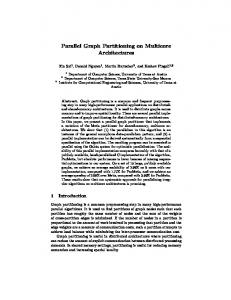
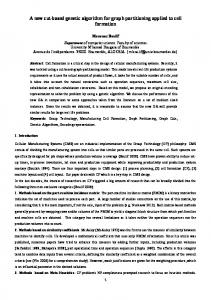
is based on direct experimental comparison using a variety of meshes. We have selected one representative test for this paper, a finite element meshing of a multi-element airfoil provided by Barth [1]. A more comprehensive reporting of our experimental results is contained in the follow on paper [10]. The airfoil mesh is shown in Figure 1 and its dual is shown in Figure 2. The dual has a vertex representing each element in the mesh (triangular faces in this case) and an edge connecting vertices representing elements which share an edge in the mesh. There are 8034 vertices and 11513 edges in this dual graph. The dual is relevant because in many parallel finite element codes, data is organized by assigning collections of individual elements to each processor. The iterative solution of the resulting equations then involves some computation associated with each element and some communication between elements sharing an edge or vertex. The dual graph therefore provides a better model for the iterative solution than the original mesh does. For ease of comparison with other methods, we chose to partition an instance of the dual in which all vertex and edge weights are equal to 1,
Fig.
1. Multi-element
airfoil mesh.
Table 8 shows the results obtained by applying various partitioning methods to The methods are listed in rank order the dual of the multi-element airfoil graph. by hop-weight, which has been shown to closely correlate with the overhead due to 15
Fig.
2. Dual of multi-element
airfoil mesh.
communication for the applications we are targeting [9]. A brief discussion of some important aspects of the partitioning algorithms follows K L refers to a recursive application of a version of the classic graph bisection heuristic devised by Kernighan and Lin [12]. KL must be supplied with an initial partition which is then improved by a greedy local strategy. We used an x-coordinate bisection of the vertices of the dual as an initial guess since this produced better partitions than any of the random initial guesses we tried. KL is a quick, linear time algorithm but is sensitive to the numbering of the vertices, and tends to do poorly on large problems because it only considers very local information about the graph. As with all bisection algorithms, one bit in the final processor assignment of a given vertex is determined at a time, so this algorithm makes no effort to minimize hops. It is clearly possible to add a phase to a bisection algorithm or any recursive partitioning algorithm which does try to further minimize hops by choosing an advantageous permutation of the set assignments of subgraphs. One such pivoting algorithm was detailed by Hammond [9]. We have used any pivoting strategy in our experiments. The inertial method recently proposed by Nour-Omid [18] is also a recursive bisection method. It treats the mesh as a rigid structure and makes cuts orthogonal to the principle axis of the structure. This is also a fast algorithm which can be implemented to run in linear time, but requires geometric information which may be unavailable and, 16
8 Processors Method
cuts
hops
cuts
hops
KIA
300
458
1158
2183
317 212
396 286
1166 997 1030 1018 911
1855 1661 1626 1463 1287
Inertial R.S13
Tablel.
64 Processors
RSQ 221 224 IWO 197 200 L RSOKL4 Performance ofdifferent partitioning multi-element airfoil mesh.
algorithms
ondual
of the
as the table indicates, it produces partitions of only moderate quality. Recursive Spectral Bisection (RSB) is the name given by Simon to the d = 1 spectral partitioning algorithm studied by him and others [18]. It requires no geometric information, is order insensitive and makes more sophisticated use of global information than the inertial method or KL. It produces much better partitions of large graphs than KL or inertial, but has an O(n@) runtime dominated by the Lanczos iteration used to find the bisecting eigenvectors. Simon [18] and Williams [21] have both concluded that RSB is preferable to several partitioning strategies not considered here. Recursive Spectral Quadrisection (RSQ) is our d = 2 spectral partitioning algorithm. Here two bits in the final processor assignment are determined concurrently to approximately minimize hops in the corresponding two hypercube dimensions. This can beat the expense of a slight increase in the cut-weight, as the table indicates. Generally only a marginal number of additional I,anczos iterations are required to compute the second eigenvector, so RSQ is actually cheaper than two levels of RSB. In fact, if we assume that the cost of the eigenvector calculation is proportional to nfi (which is appropriate for the Lanczos procedure [14]), then a single step of RSQ is faster than two steps of RSB by a factor of 1 + fi/2. There is no 8 processor entry for RSQ because it is not possible to partition into 8 sets with an integral number of quadrisection steps. Recursive Spectral Octasection (RSO) is our d = 3 spectral partitioning algorithm which approximately minimize-s hops in three hypercube dimensions at a time. In general it produces partitionings with fewer hops and perhaps slightly more cuts than RSQ and RSB, although it happens to do better on cuts than RSQ in this case. It is also cheaper than both RSQ and RSB. Assuming again that the eigenvector calculations cost O(n@), one step of RSO is faster than three steps of RSB by a factor of (3 + ti)/2. The last algorithm, RSOKL, is a composite algorithm in which the output of RSO at each stage of recursion is fed into a generalized KL algorithm capable of minimizing hops over an 8 way initial partitioning. The motivation for this strategy was to combine the global strength of RSO with the local finesse of KL. The resulting partition is clearly the best with respect to both cuts and hops. The KL phase of the algorithm accounts for only a small portion of the run time, so the net cost of RSOKL is substantially less than that of RSB. Notice that for the 8 processor case the cut and hop totals are nearly equal, indicating that almost all communication occurs between adjacent processors. 17
KL can be appended to the other algorithms as well, but we have found RSOKL to be the best combination given our communication metric. RSOKL is discussed in more detail in [10]. RSO and RSQ can also be more robust than RSB when the graph exhibits symmetry. For example, the three-fold symmetry of the cubic grid-graph causes A~ of its Laplacian to have a multiplicity of three, and the corresponding eigenspace to be three-dimensional. Since RSB chooses a single vector from this subspace essentially at random, it may fail badly. It will, for example, make a diagonal cut through the grid for some Lanczos starting vectors. In contrast, RSO works within the entire subspace, rotating the basis vectors in such a way that it returns a gray-coding of blocks of the grid. This is the optimal result in which cuts and hops are as small as possible and all communication is between adj scent processors. To demonstrate that this discrepancy does arise in practice, we ran both methods on a simple 4 x 4 x 4 grid graph. In RSB we used the Lanczos starting vector recommended by Pothen, Simon and Lieu [15], namely ri = i —(n+ 1)/2, and iterated until the eigenresidual Au – Au was below 10–6. The resulting decomposition had 72 cuts and 78 hops. In RSO we solved to the same accuracy for this starting vector and several random starting vectors. In each case we obtained 48 cuts and 48 hops, the optimal partitioning. Similar results may be observed with other symmetric graphs. 9. Conclusions. We have presented a method for mapping large problems onto the nodes of a hypercube multiprocessor in such a way that the computational load is balanced and the communication overhead is kept small. For the problems we have investigated, this approach generates mappings that have lower communication requireBecause the 2nd and 3rd eigenvcctors are ments than other partitioning techniques. relatively inexpensive to calculate, the net cost of spectral quadrisection or octasection is significantly less than that of spectral bisection. In addition, our method yields computable lower bounds for the communication cost of any balanced partitioning scheme which are tighter than those previously known. Although our method was developed with a hypercube communication network in mind, this approach should work well for other machine topologies. For example, a t we-dimensional mesh can be defined as a collection of t we-dimensional hypercubes, so a recursive application of our quadrisection approach is immediately applicable. Similarly, a three-dimensional mesh is composed of three-dimensional hypercubes, so our octasection algorithm can be applied. For other architectures we expect our approach to be useful as a heuristic. Although the method tries to minimize a communication function that counts hypercube hops, in practice the spectral quadrisection and octasection algorithms divide a domain into pieces that require a small communication volume. This should lead to low communication overhead on most parallel machines. Graph partitioning also finds application in network design, circuit layout, sparse matrix computations and a number of other disciplines. Consequently, the partitioning algorithm we have described may find uses far afield from parallel computing. More broadly, the way we have made use of multiple eigenvectors is, to our knowledge, unlike any previous work in spectral graph theory. It is our hope that these ideas can be 18
applied to other spectral
graph theoretic
problems.
The ideas in this paper have evolved through discussions with many people including Horst Simon, Alex Pothen, Louis Romero, Ray Tuminaro, John Shadid and Steve Plimpton. Acknowledgements.
REFERENCES [1] T. BARTH. [2] R. BOPANA,
Personal Communication, December 1991. Eigenvalues and graph bisection: An average case analysis, in Proc. 28th Annual
Symposium on Foundations of Computer Science, IEEE, 1987, pp. 280-285. Algorithms for partitioning of graphs and computer logic based [3] W. DONATH AND A. HOFFMAN, on eigenuectors o~connection makices, IBM Technical Disclosure Bulletin, 15 (1972), pp. 938– 944. [4] —, Lower bounds for the partitioning of graphs, IBM J. Res. Develop., 17 (1973), pp. 420-425. [5] M. FIEDLER, Algebmic connectivity of graphs, Czechoslovak Math. J., 23 (1973), pp. 298-305. [6] — A property of eigenvectors of nonnegative symmetric matrices and its application to graph th’eory, Czechoslovak Math. J., 25 (1975), pp. 619-633. John [7] R. FLETCHER, Practicai Methods OJ Optimization, Volume 2, Constrained Optimization, Wiley & Sons, New York, 1986. D. JOHNSON, AND L. STOCKMEYER, Some simplified NP-complete graph problems, [8] M. GAREY, Theoretical Computer Science, 1 (1976), pp. 237-267. Mapping unstructured grid computations to massively parallel computers, PhD [9] S. HAMMOND, thesis, Rensselear Polytechnic Institute, Dept. of Computer Science, Renssealear, NY, 1992. AND R. LELAND, Domain mapping of parallel scientific computations, Tech. [10] B. HENDRICKSON Rep. SAND 92-1461, Sandia National Laboratories, Albuquerque, NM, 1992. Numerical methods for unconstrained optimization [11] J. J. DENNIS AND R. SCHNABEL,
[12] B. [13]
B.
[14] B. [15] A. [16] D.
[17] F.
[18] H.
[19] P. [20] T. [21] R. [22] D.
and nonlinear equations, Prentice-Hall, Inc., Englewood Cliffs, NJ, 1983. KERNIGHAN AND S. LIN, An eficient heuristic procedure for partitioning graphs, Bell System Technical Journal, 29 (1970), pp. 291-307. MOHAR, The Laplacian spectrum of graphs, in 6th International Conference on Theory and Applications of Graphs, Kalamazoo, Ml, 1988. PARLETT, The Symmetric Eigenvalue Problem, Prentice-Hall, Englewood Clif7s, NJ, 1980. POTHEN, H. SIMON, AND K. LIOU, Partitioning sparse matrices with eigenuectors oj graphs, SIAM J. Matrix Anal., 11 (1990), pp. 430-452. POWERS, Graph partitioning by eigenvectors, Lin. Alg. Appl., 101 (1988), pp. 121-133. RENDL AND H. WOLKOWICZ, A projection technique for partitioning the nodes of a graph, Tech. Rep. CORR 90-20, University of Waterloo, Faculty of Mathematics, Waterloo, Ontario, November 1990. SIMON, Partitioning of unstructured problems for parallel processing, in Proc. Conference on Parallel Methods on Large Scale Structural Analysis and Physics Applications, Pergammon Press, 1991. SUARIS AND G. KEDEM, An algorithm for quadrisection and its application to standard cell placement, IEEE Trans. Circuits and Systems, 35 (1988), pp. 294-303. TOKUYAMA AND J. NAKANO, Geometric algorithms fora minimum cost assignment problem, in Proc. 7th Annual Symposium on Computational Geometry, ACM, 1991, pp. 262–271. WILLIAMS, Performance of dynamic load balancing algorithms for unstructured mesh calculations, Concurrency, 3 (1991), pp. 457-481. WOMBLE, A time-stepping algorithm for parallel computers, SIAM J. Sci. Stat. Comput., 11 (1990), pp. 824-837.
19
, DISTRIBUTION: Scott Baden University of California, Dept. of Computer Science 9500 Gilman Drive Engineering 0114 La Jolla, CA 92091-0014
San
Diego
Steve Barnard Systems Division Applied Research Branch NASA Ames Research Center Mail Stop T045-1 Moffett Field, CA 94035 NAS
Edward Barragy Dept. ASE/EM University of Texas Austine, TX 78712 M. Berzins Stool of Computer Studies The University of Leeds Leeds, LS290T United Kingdom Rob Bisseling Shell Research B.V. Postbus 3003 1003 AA Amsterdam The Netherlands Ravi Boppana Department of Computer NYU 251 Mercer Street 10012 New York, NY
Science
J. Browne University of Texas Dept. of Computer Science Taylor Hall 5.126 Austin, TX 78712 Tony Chan Department of Computer The Chinese University Shatin, NT Hong Kong
Science of Hong
Kong
Ted Charrette MIT Bldg. E3 554 42 Carleton St. Cambridge, MA 02142 Siddartha Chatterjee RIACS, NASA Ames Research Center Mail Stop T045-1 Moffett Field, CA 94035-1OOO Tom Coleman Dept . of Computer Upson Hall Cornell University Ithacar NY 14853
Science
-20-
Sean Dolan nCUBE 919 E. Hillsdale Blvd. Foster City, CA 94404 Alan Edelman University of California, Dept . of Mathematics Berkeley, CA 94720 Salvatore Filippone IBM ECSEC Viale Oceano Pacifico 00144 Roma, Italy
Berkeley
171/173
John Gilbert Xerox PARC 3333 Coyote Hill Road Palo Alto, CA 94304 Bashkar Ghosh Department of Computer Yale University POB 2158, Yale Station New Haven, CT 06520
Science
Anne Greenbaum New York University Courant Institute 251 Mercer Street New York, NY 10012-1185 Steve Hammond CERFACS 42 Ave Gustave 31057 France
Toulouse
Coriolis Cedex
Mike Heath University of Illinois 4157 Beckman Institute 405 N. Mathews Ave. Urbana, IL 61801 Greg Heileman EECE Department University of New Mexico Albuquerque, NM 87131 A.J. Hey University of Southampton Dept . of Electronics and Computer Mountbatten Bldg., Highfield Southampton, S09 5NH United Kingdom
Science
Adolfy Hoisie Cornell University Cornell Theory Center 631 E&TC Bldg Ithacar NY 14853 Graham Horton Universitat Erlangen-Nurnberg IMMD III Martensstrase 3 8520 Erlangen, FRG
-21-
Kapil Mathur Th;nking Machines Corporation 245 First Street Cambridge, MA 02142-1214 William McCO1l Oxford University 8-11 Keble Road Oxford, OX1 3QD United Kingdom
Computing
Robert McLay University of Texas Dept . ASE-EM Austin, TX 78712
Laboratory
at Austin
Jill Mesirov Thinking Machines Corporation 245 First Street Cambridge, MA 02142-1214 Bojan Mohar Department of Mathematics University of Ljubljana Jadranska 19, 61111 Ljublajana Slovenia Can Ozturan Department of Computer Rensselaer Polytechnic Troy, NY 12180
Science Institute
Glauscio Paulino Civil Engineering Cornell University Hollister Hall 413 Ithaca, NY 14853 Paul Plassman Math and Computer Science Argonne National Lab Argonne, IL 60439
Division
Alex Pothen Computer Science Department University of Waterloo Waterloo, Ontario N2L 3G1 Canada Mike Quayle Cadence Design Systems 2 Lowell Research Center Lowell, MA 01857 Sanjay Ranka School of Computer and Suite 4-116 Center for Science and Syracuse, NY 13244-4100 Satish Rao NEC Research Institute, 4 Independence Wayr Princeton, NJ, 08540
Drive
Information
Science
Technology
-22-
Franz Rendl Technische Universitat Graz Institute fur Mathematik Kopernikusgasse 24, A-901O Graz,
Austria
John Richardson Thinking Machines Corporation 245 First Street Cambridge, MA 02142-1214 John Rollett Oxford University 8-11 Keble Road Oxford, OX1 3QD United Kingdom
Computing
Laboratory
Diane Rover Michigan State University Dept . of Electrical Engineering 260 Eng. Bldg. East Lansing, MI 48824 Margaret St, Pierre Thinking Machines Corporation 245 First Street Cambridge, MA 02142-1214 Joel Saltz Computer Science Department A.V. Williams Building University of Maryland College Park, MD 20742 Rob Schreiber RIACS NASA Ames Research Mail Stop T045-1 Moffett Field, CA
Center 94035-1OOO
Horst Simon NAS Systems Division Applied Research Branch NASA Ames Research Center Mail Stop T045-1 Moffett Field, CA 94035 Richard Sincovec Oak Ridge National Laboratory 2008, Bldg 6012 P.O. BOX Bethel Valley Road TN 37831-6367 Oak Ridge, Anthony Skjellum Lawrence Livermore National Laboratory 7000 East Ave.r Mail Code L-316 Livermorer CA 94550 Burton Smith Tera Computer Co 400 N. 34th St., Suite Seattle, WA 98103 Mike Stevens nCUBE 919 E. Hillsdale Foster City, CA
300 .
Blvd. 94404
-23-
Judy Sturtevant Mission Research Corporation 1720 Randolph Rd. SE NM 87106-4245 Albuquerque, Shari Trewin Edinburgh Parallel Computing The University of Edinburgh Janes Clerk Maxwell Bldg. The King’s Buildings Mayfield Road Edinburgh, EH9 3JZ United Kingdom Ray Tuminaro CERFACS 42 Ave Gustave 31057 Toulouse France
Centre
Coriolis Cedex
Stefan Van de Wane Katholieke Universiteit Leuven Dept. of Computer Science Celestjnenlaan 200A B-3001 Leuven, Belgium John Van Rosendale ICASE, NASA Langley MS 132C Hampton, VA 23665 Steve Vavasis Dept . of Computer Upson Hall Cornell University Ithacar NY 14853
Research
Center
Science
C. Walshaw School of Computer Studies University of Leeds Leeds LS2 9JT United Kingdom Robert Weaver University of Colorado at Boulder Dept . of Computer Science Campus Box 430 Boulder, CO 80309 Roy Williams California Institute 206-49 Pasadena, CA 91104
of Technology
Henry Wolkowicz Department of Combinatorics University of Waterloo Waterloo, Ontario, N2L 3G1 Canada
Paul Fleury Ed Barsis
1000 1400
and
Optimization
-24-
Sudip Dosanjh Bill Canp Doug Cline David Gardner Grant Heffelfinger Scott Hutchinson Martin Lewitt Steve Plimpton Mark Sears John Shadid Julie Swisshelm Dick Allen Bruce Hendrickson (15) David Womble Ernie Brickell Robert Benner Carl Diegert Art Hale Rob Leland (15) Courtenay Vaughan Steve Attaway Johnny Biffle Mark Blanford Jim Schutt Michael McGlaun Allen Robinson Paul Barrington David Martinez Dona Crawford William Mason Technical Library (5) Technical Publications Document Processing for DOE/OSTI (10) Central Technical File Charles Tong
1402 1421 1421 1421 1421 1421 1421 1421 1421 1421 1421 1422 1422 1422 1423 1424 1424 1424 1424 1424 1425 1425 1425 1425 1431 1431 1432 1434 1900 1952 7141 7151 7613-2 8523-2 8117
-25-