An improved version of the view factor method for simulating inertial confinement fusion hohlraums Mikhail Baskoa) Max-Planck-Institut fu¨r Quantenoptik, D-85748 Garching, Germany
~Received 17 April 1996; accepted 5 August 1996! A modified version of the view factor equations is proposed which improves the accuracy of the description of temporal effects in energy redistribution by thermal radiation in cavities driven by power pulses typical for inertial confinement fusion ~ICF!. The method is applied to analyze the process of radiative symmetrization in the simplest type of closed cylindrical hohlraums heated by two x-ray rings on the sidewall of the hohlraum case. Such hohlraums may be used in certain types of ICF targets driven by ion beams. © 1996 American Institute of Physics. @S1070-664X~96!02411-1#
I. INTRODUCTION
II. VIEW FACTOR EQUATIONS
Indirect drive approach to inertial confinement fusion ~ICF! is based on the concept of radiation cavity—a hohlraum.1 The driving laser or particle beams generate thermal x rays inside a high-Z cavity case. These x rays are repeatedly absorbed and reemitted by the case walls and deposit their energy upon the surface of a spherical fusion capsule inside the hohlraum in a nearly perfectly symmetric way. However, for any particular type of an ICF target, the hohlraum configuration must be carefully designed to provide the necessary symmetry of capsule irradiation.2 An effective practical method for calculating radiative energy redistribution in hohlraums, particularly suitable for the initial stage of hohlraum optimization, is based on a ‘‘view factor’’ approach.3–6 A major drawback of the original system of the view factor equations, as proposed in Refs. 3–6, is associated with poor accuracy in describing temporal effects for non-powerlaw variations of the source power. In Sec. II it is shown how these equations can be modified to render a much more accurate description of hohlraums with sudden increases of the driving power. Section III describes briefly how the values of the reemission parameters, which enter the view factor equations, can be calculated for different materials. In Sec. IV, the modified system of the view factor equations is applied to analyze the temporal behavior of the loworder asymmetry modes in closed cylindrical hohlraums heated by two ring sources of x rays. Such hohlraums may provide an interesting option for ICF targets driven by the beams of heavy ions.7,8 The time-dependent effects due only to multiple reemission by the hohlraum walls and capsule surface are analyzed. The neglect of the plasma blowoff effects is partly justified by relatively large hohlraum dimensions considered. To make an easy comparison with the laser target proposed for the National Ignition Facility ~NIF!,2 a fusion capsule of the same size R c 51.11 mm, and the x ray pulse of approximately the same shape and the same energy as in the NIF target are used in all the numerical simulations. a!
On leave from the Institute for Theoretical and Experimental Physics, B. Cheremushkinskaya 25, 117259 Moscow, Russia. Electronic mail:
[email protected]
4148
Phys. Plasmas 3 (11), November 1996
The view factor equations express the energy balance for each surface element inside a radiation cavity in the form S a ~ t,r! 1S r ~ t,r! 5S q ~ t,r! 1
E
A
V f ~ r,r8 ! S r ~ t,r8 ! dA 8 , ~1!
where S a ~t,r! and S r ~t,r! are, respectively, the fluxes of the absorbed and reemitted radiation ~per unit surface area!, S q ~t,r! is the radiation flux received from the external sources, and dA 8 is the surface element at point r8 ~for more details see Ref. 6!. Under the assumption of Lambertian ~isotropic! reemission, the view vactor V f ~r,r8! is given by V f ~ r,r8 ! 52
~ l–n!~ l–n8 ! , p u lu 4
~2!
where l5r82r, and n and n8 are the unit normal vectors to the surface elements at r and r8, respectively. To solve the integral equation ~1!, it was originally proposed5,6 to use a power law relationship S r ~ t,r! 5K r t a 8 @ S a ~ t,r!# b 8
~3!
between the absorbed, S a , and the reemitted, S r , fluxes; here K r , a8, and b8 are certain constants characterizing the wall material. This relationship stems from the family of selfsimilar solutions for a planar wall, either static9 or undergoing hydrodynamic expansion,10 which is heated by an external thermal bath with temperature T ex(t) varying as a certain power of t. Evidently, Eq. ~3! may become very inaccurate when the time variation of T ex deviates from the power law, with a typical example of T ex remaining more or less constant for a certain period of time ~like during the foot of the driving pulse in indirect drive ICF targets2! and then rising suddenly to a new value, which persist for some time later. Here it is demonstrated that the accuracy of the view factor method can be improved dramatically if, instead of Eq. ~3!, one uses the equations S r ~ t,r! 5K r @ E a ~ t,r!# a @ S a ~ t,r!# b ,
~4!
] E a ~ t,r! 5S a ~ t,r! , ]t
~5!
1070-664X/96/3(11)/4148/8/$10.00
© 1996 American Institute of Physics
Downloaded¬27¬Jun¬2009¬to¬140.181.70.110.¬Redistribution¬subject¬to¬AIP¬license¬or¬copyright;¬see¬http://pop.aip.org/pop/copyright.jsp
FIG. 1. ~a! Time dependence of the boundary temperature T ex for the test problem ~6!–~10!. ~b! Ratio between the reemitted S r and the absorbed S a energy fluxes as calculated ~i! by numerically solving Eq. ~6!—black dots, ~ii! in the tS approximation—dashed curve, and ~iii! in the ES approximation—solid curve.
to relate S r and S a . Below we refer to Eq. ~3! as a ‘‘tS’’ approximation, and to Eqs. ~4! and ~5! as an ‘‘ES’’ approximation. As an illustrative example, consider penetration of a planar heat wave into a motionless wall ~hydrodynamic expansion is not relevant for the present argument: when accounted for, it only changes the values of K r , a, and b! heated by an external source with temperature T ex(t) which varies in time as shown in Fig. 1~a!. In many cases of practical interest such a heat wave can be described by the heat conduction equation
S
D
]Tm ] ]T 5 e k Tn , * ]t * ]x ]x
~6!
m
where e T is the specific ~per unit volume! energy of the * wall material, and k T n is the heat conduction coefficient. * When a boundary condition S a ~ t ! [2 k T n
*
]T ]x
U
5S 0 t q
~7!
x50
is imposed, Eq. ~6! admits a self-similar solution which yields the reemitted flux in the form S r ~ t ! [ s T 4 ~ t,0! 5 s¯ T 40
S S
tS 2a ~ t ! ~ q11 ! e k
D
4/~ n1 m 11 !
* * E a ~ t ! S a ~ t ! 4/~ n1 m 11 ! 4 ¯ 5sT0 , ~8! e k * * where s is the Stefan–Boltzmann constant, and ¯ ¯ ( m ,n,q) is a slowly varying dimensionless parameter T 0 5T 0
D
Phys. Plasmas, Vol. 3, No. 11, November 1996
FIG. 2. The same as Fig. 1 but for the boundary temperature T ex(t) varying as shown in part ~a! of this figure.
that should be calculated by solving numerically the eigenvalue problem for the ordinary differential equation to which Eq. ~6! is reduced. For the case of m51, n54, q521/2 considered below, ¯ T 051.329. One can use either the ‘‘tS’’ form of Eq. ~8! to find the values of K r , a8, and b8 for the Eq. ~3!, or its ‘‘ES’’ form to determine the values of K r , a, and b for the Eq. ~4!. Figure 1~b! shows the comparison between the tS and ES approximations for a particular case of s5k 5e 5m51. * * The exponent q in Eq. ~7! was set equal to 21/2, so that the T ex(t)5constant phase is reproduced exactly by both the tS and ES approximations. As a result, in the tS approximation we calculate ¯3 A2tT ~ t ! S ~ t ! /S ~ t ! 5T ~9! r
a
0
ex
@the dashed line in Fig. 1~b!#, while the ES equations yield
SE
¯3 T 22 ~ t ! 2 S r ~ t ! /S a ~ t ! 5T 0 ex
t
0
T 6ex~ t 8 ! dt 8
D
1/2
~10!
@the solid line in Fig. 1~b!#. The black dots in Fig. 1~b! represent the numerical solution of the partial differential equation ~6! with the boundary temperature as given in Fig. 1~a!. One clearly sees that at times 1,t&1.5 the error of the tS approximation is in excess of 100%, while the ES curve is hardly distinguishable from the solution of the diffusion equation ~6!. Figure 1 illustrates one characteristic example of a nonpower-law time dependence of the source power, when it rises steeply to a new level. Intuitively, it is clear that the ES method will be always superior to the tS approximation in any such situation simply because the absorbed energy E a is a better measure of the diffusive saturation of the heat wave with respect to the new power level than the time t elapsed from the initial power onset. Figure 2 shows another characMikhail Basko
4149
Downloaded¬27¬Jun¬2009¬to¬140.181.70.110.¬Redistribution¬subject¬to¬AIP¬license¬or¬copyright;¬see¬http://pop.aip.org/pop/copyright.jsp
TABLE I. Equation-of-state, opacity, and reemission parameters for a selection of elements with different Z. Parameter
Be
C
Al
Fe
Au
e ~10 g cm s keV ! * l (g n R cm12 n R keV2 m R ) * m n mR nR
9.4 50 1.0042 0.0024 3.9 1.8
11.1 70 1.025 0.013 5.5 1.8
12.5 5.0 1.145 0.063 3.8 1.5
14.2 0.0027 1.327 0.120 0.58 1.32
11.5 0.003 1.525 0.157 1.25 1.2
¯ T0
1.032
1.057
1.079
1.078
1.113
Kr a b
0.47 0.395 0.714
1.21 0.339 0.620
1.34 0.399 0.648
5.08 0.573 0.881
14.1 0.510 0.748
14
n
2m
223n 22
teristic case, when the initially steep rise of the external temperature, T ex(t)}t 1/2 @q51 in Eq. ~7!#, is followed by a plato with T ex(t)5constant. Again, the advantage of the ES approximation is quite conspicuous. A test case with a sudden drop of the source power would be of no practical interest because both the tS and ES approximations fail to reproduce the behavior of the reemission factor S r /S a under such conditions, when the absorbed flux S a becomes very low and a heated wall radiates back its stored energy. III. REEMISSION COEFFICIENTS
The values of the reemission parameters K r , a, and b in Eq. ~4! can be determined by either fitting the results of one-dimensional numerical simulations of radiatively driven ablation waves,4 or by using a suitable self-similar solution. Here we use the Pakula–Sigel10 self-similar solution, which describes an ablation wave driven into an initially dense planar wall by radiative heat conduction. In contrast to the simple conduction equation ~6!, this solution accounts for the effect of hydrodynamic expansion on the reemission properties of an ablated surface. Equations of hydrodynamics with radiative heat conduction admit a self-similar solution when the equation of state and the Rosseland mean free path are approximated as power law functions of temperature and density:
e5
pV 5 e T mV n, * g 21
~11!
l R 5l T m R V n R .
~12! * Here e is the specific internal energy, p is the pressure, T is the temperature, V[1/r is the specific volume, g511n/ ~m21! is the adiabatic index, e , l , m, n, mR , and nR are * * the fit parameters. From pure dimensional considerations, one can obtain the following expression for the reemitted radiation flux: T 40 S r 5 s¯
FS D Ea k
12 ~ 3/2! n
e
*
G
4L n 2 ~ 1/2! n S aR , ~ 3/2! n R 2 ~ 1/2!
*
~13!
where 16 k 5 sl , * 3 *
4150
L5
2 , ~ 223 n !~ m R 14 ! 1 m ~ 3 n R 21 ! ~14!
Phys. Plasmas, Vol. 3, No. 11, November 1996
and ¯ T 0 is a dimensionless constant that should be determined by solving numerically the corresponding eigenvalue problem. Below we use the value of ¯ T 0 calculated for a constant value of the absorbed flux S a . This particular case of the Pakula–Sigel solution is appropriate for closed hohlraums heated by ion beams, whereas open hohlraums driven by laser beams might be more adequately described by a solution with a constant boundary temperature, i.e., by somewhat different value of ¯ T 0 . From Eq. ~13! one calculates readily the values of K r , a, and b that are needed in the Eq. ~4!. Note that, in their original publication, Pakula and Sigel used the equation of state with n50, which is thermodynamically inconsistent for mÞ1. Table I lists the values of the fit parameters in Eqs. ~11! and ~12! as calculated for the temperature and density intervals 100 eV