Jun 26, 2017 - We make two assumptions in our analysis of IQN, both of which are ..... error of 10â10 after 10 passes through the data while SAGA achieves the .... 2016, available at http://www.seas.upenn.edu/â¼maeisen/wiki/incr-bfgs-.
AN INCREMENTAL QUASI-NEWTON METHOD WITH A LOCAL SUPERLINEAR CONVERGENCE RATE Aryan Mokhtari
Mark Eisen
Alejandro Ribeiro
Department of Electrical and Systems Engineering, University of Pennsylvania
ABSTRACT We present an incremental Broyden-Fletcher-Goldfarb-Shanno (BFGS) method as a quasi-Newton algorithm with a cyclically iterative update scheme for solving large-scale optimization problems. The proposed incremental quasi-Newton (IQN) algorithm reduces computational cost relative to traditional quasi-Newton methods by restricting the update to a single function per iteration and relative to incremental second-order methods by removing the need to compute the inverse of the Hessian. A local superlinear convergence rate is established and a strong improvement is shown over first order methods numerically for a set of common large-scale optimization problems. Index Terms— Stochastic optimization, quasi-Newton, incremental method, superlinear convergence 1. INTRODUCTION We study a large scale optimization problem where we seek to minimize an objective function that is an aggregation of many component objective functions. To be more precise, consider a variable x ∈ Rp and a function f which is defined as the average of n strongly convex functions labelled fi : Rp → R for i = 1, . . . , n. Our goal is to find the optimal point x∗ as the solution to the problem x∗ = argmin f (x) := argmin x∈Rp
x∈Rp
n 1X fi (x), n i=1
(1)
in a computationally efficient manner even when n is large. Problems of this form arise in machine learning [1–4], control problems [5–7], and wireless communication [8–10]. Much of the theory that has been developed to solve (1) is centered on the use of iterative descent methods. For large scale machine learning and optimization settings, n can be very large and the full gradient is often too costly to compute at each iteration. As an alternative, stochastic methods seek to find a solution to (1) while computing only a subset of the total n gradients at each iteration, thus significantly reducing the computational burden. The simplest version of a stochastic algorithm is stochastic gradient descent (SGD), which at each time step t draws a random index it and performs a descent using the gradient of only a single function [2]. More sophisticated stochastic first order methods use variance-reduced gradients (e.g. SVRG [11]) or averaging gradients (e.g. SAG [12, 13], SAGA [14]) to reduce computation cost while retaining a linear convergence rate. Moving beyond first order information, there have been stochastic quasi-Newton methods to approximate Hessian information [15–19]. All of these stochastic quasi-Newton methods reduce computational cost of quasi-Newton methods by updating only a randomly chosen single or small subset of gradients at each iteration. However, they are not able to recover the superlinear convergence rate of quasi-Newton methods [20–22]. Alternatively to stochastic methods are incremental methods, which deterministically iterate through all component functions in a cyclic fashSupported by NSF CAREER CCF-0952867 and ONR N00014-12-1-0997.
ion, again only computing a single gradient or Hessian per iteration. Incremental methods have been used with both aggregated gradients [23, 24] and second-order Hessian information [25, 26] . The incremental Newton method (NIM) in [26] is the only incremental method shown to have a superlinear convergence rate; however, the Hessian function is not always available or computationally feasible. Moreover, the implementation of NIM requires computation of the incremental aggregated Hessian inverse which has the computational complexity of the order O(p3 ). We propose an incremental variant of BFGS which achieves a greater local convergence rate than that of first order incremental or stochastic methods while reducing the computational cost per iteration to O(p2 ) by using an incremental aggregated approximation of the Hessian. We begin with the paper by introducing the well-known BFGS method and its update for solving (1) (Section 2). While incremental methods have been used in first order methods, they achieve only a linear convergence rate. We introduce an incremental quasi-Newton (IQN) method that requires only computing a single gradient and Hessian approximation per iteration (Section 3). The proposed IQN method uses an approximation of second-order information that requires less cost than computing the Hessian inverse directly while maintaining its superior analytical and numerical performance. The local superlinear convergence of IQN is established (Section 4) and performance advantages relative to first order stochastic and incremental methods are evaluated numerically (Section 5). Proofs for results presented are found in [27]. 2. BFGS QUASI-NEWTON METHOD Consider the problem in (1) for a relatively large n. In a conventional optimization setting, it can be solved using a descent method, such as gradient descent or Newton’s method, which iteaitivley updates a variable xt for t = 0, 1, . . . using the general recursive expression xt+1 = xt + η t dt ,
(2)
where η t is a scalar step size and dt is the descent direction at time t— defined as either dt := −∇f (xt ) or dt := −(∇2 f (xt ))−1 ∇f (xt ) for gradient descent and Newton’s method, respectively. In both cases, iterations xt converge to the optimal solution x∗ . Gradient descent, however, using only the first-order information contained in the gradient converges at a linear rate while Newton’s method, using second-order information in the Hessian, converges at a significantly faster quadratic rate [28]. In the case that the Hessian information required in Newton’s method is either unavailable or too costly to evaluate, quasi-Newton methods have been developed to approximate second-order information to improve upon the convergence rate of first order methods [20]. Quasinewton methods perform an update using a descent direction of the form dt := −(Bt )−1 ∇f (xt ), where Bt is an approximation of the Hessian ∇2 f (xt ). There are different approaches to approximate the Hessian, with the most popular being the method of Broyden-Fletcher-GoldfarbShanno (BFGS) [20–22]. In BFGS, two auxiliary variables are defined to capture difference in variables and gradients of successive iterations, i.e. st := xt+1 − xt ,
yt := ∇f (xt+1 ) − ∇f (xt ).
(3)
Then, given the variable variation st and gradient variation yt , the Hessian approximation is updated using the recursive equation T
Bt+1 = Bt +
T
yt yt Bt st st Bt − . T yt st st T Bt st
(4)
The BFGS method is popular not only for its strong numerical performance relative to the gradient descent method, but also because it is shown to exhibit a superlinear convergence rate [20], thereby providing a theoretical guarantee of superior performance. In fact, it can be shown that, for the BFGS update the equation lim
t→∞
k(Bt − ∇2 f (x∗ ))st k =0 kst k
(5)
known as the Dennis-Mor´e condition, which is both necessary and sufficient for superlinear convergence [22], is satisified. This result solidifies quasi-Newton methods as a strong alternative to first order methods when exact second-order information is unavailable. 3. INCREMENTAL QUASI-NEWTON METHOD We introduce a novel incremental quasi-Newton (IQN) algorithm, in which the updated gradient information of only a single function fi is updated at each iteration. Consider that each component Hessian ∇2 fi (xt ) is approximated with Bti and define n copies of the variable xt , notated as zt1 , zt2 , . . . , ztn , each corresponding to a different function fi . In particular, zti shows the vector x at the last time before step t that function fi is chosen to update descent direction. We define the update of Hessian approximation Bti using the traditional BFGS update in (3)-(4), but instead using the i-th copies zti and zt+1 in place of xt and xt+1 . We redefine the variable and gradient difi ferences associated with the function fi as sti := zt+1 − zti i
yit := ∇fi (zt+1 ) − ∇fi (zti ), i
(6)
Note that if at step t + 1 and t − τ , where τ ≥ 0, the function fi is chosen for updating the gradient information, then we have zt+1 = xt+1 i t t−τ and zi = x . In particular, if we use a cyclic scheme for choosing the functions we have τ = n − 1, i.e., zti = xt−n+1 . This observation shows that the variable and gradient variation defined in (6) can be written as ) − ∇fi (xt−τ ). Therefore, sti := xt+1 − xt−τ and yit := ∇fi (xt+1 i i these definitions are different from the ones for classic BFGS in (3)-(4). Likewise, the Hessian approximation of the IQN is different from BFGS in using sti and yit instead of st and yt . Thus, the Hessian approximation Bti corresponding to the function fi is updated as Bt+1 = Bti + i
t Bti sti stT yit yitT i Bi − . t t yitT sti stT i Bi si
(7)
To derive the full variable update, we use an approach similar to that used in the Newton-type Incremental Method (NIM) [26]. Consider the second-order approximation of the function fi (x) centered around zti as fi (x) ≈ fi (zti ) + ∇fi (zti )T (x − zti ) 1 + (x − zti )T ∇2 fi (zti )(x − zti ). 2
(8)
As in traditional quasi-Newton methods, we replace the i-th Hessian ∇2 fi (zti ) by Bti . Using the approximation P matrices in place of Hessians, the objective function f (x) = (1/n) n i=1 fi (x) can be approximated with f (x) ≈
n n 1X 1X fi (zti ) + ∇fi (zti )T (x − zti ) n i=1 n i=1
+
n 1X1 (x − zti )T Bti (x − zti ). n i=1 2
(9)
Considering the approximation in (9), we approximate the optimal argument of f (x) by the optimal argument of the function (9). Thus, we deP Pin n t t T ˆ t+1 := argmin{(1/n) n f (z fine x )+(1/n) i i i=1 i=1 ∇fi (zi ) (x− Pn t T t t t zi ) + (1/2n) i=1 (x − zi ) Bi (x − zi )} as the auxialiary variable at iteration t + 1. Solving this quadratic programming yields the following ˆ t+1 closed-form update for the variable x t+1
ˆ x
=
n 1X t Bi n i=1
!−1 "
# n n 1X t t 1X t Bi zi − ∇fi (zi ) . n i=1 n i=1
(10)
As in traditional descent methods, we introduce a step size 0 ≤ η t ≤ 1 and define the variable xt+1 corresponding to step t + 1 as the weighted average of the previous iterate xt and the evaluated auxiliary variable ˆ t+1 , i.e., x ˆ t+1 + (1 − η t )xt . xt+1 = η t x
(11)
From here, it remains to show how the individual variable copies zti and Hessian approximations Bti are updated. We use a cyclic update scheme to remove the need to compute all gradients and Hessian approximations at each iteration. Therefore, if we define it as the index of the function chosen at step t, it is updated by cyclically iterating through all indices in order, i.e., it = {1, 2, . . . , n, 1, 2, . . .}. At time t, we update the variable copies as zt+1 = xt+1 , it
zt+1 = zti for all i 6= it . i
(12)
is changed at time t while all others are Thus only a single variable zt+1 it kept the same. Note that the variable differences in (6) will be null unless i = it and thus only one approximation Btit will change at each time t. To see that this updating scheme requires evaluation of only a single gradient and Hessian approximation matrix per iteration, consider writing the update in (17) as � ˜ t )−1 ut − gt , ˆ t+1 = (B x (13) ˜ t := Pn Bti , where we define as the aggregate Hessian approximation B i=1 Pn t t t the aggregate Hessian-variable product u := i=1 Bi zi , and the agPn t t gregate gradient g := i=1 ∇fi (zi ). Then, given that at step t only a single index is updated, we can evaluate these variables for step t + 1 as � ˜ t+1 = B ˜ t + Bt+1 B − Btit , (14) it t+1 t t+1 t+1 t t � u = u + Bit zit − Bit zit , (15) t+1 t t+1 t � g = g + ∇fit (zit ) − ∇fit (zit ) . (16) Thus, only a single Bt+1 and ∇fit (zt+1 it it ) need to be computed at each iteration, significantly reducing the computation burden of the algorithm relative to traditional quasi-Newton methods. ˜ t in (7) reduces computational Although the update of the matrix B complexity of the IQN method, the update in (13) requires computation ˜ t )−1 which has a expensive computational comof the inverse matrix (B plexity of the order O(p3 ). This extra computation cost can be avoided using the fact that the update in (7) can be simplified as t tT t t tT t ˜ t+1 = B ˜ t + yit yit − Bit sit sit Bit . B i tT t t sit Bit sit yitT stt
(17)
To derive the expression in (17) we have substituted the difference t Bt+1 it − Bit by its rank two expression in (7). By applying the ShermanMorrison formula twice to the update in (17) we can directly compute ˜ t+1 )−1 as the inverse matrix (B ˜ t+1 )−1 = Ut + (B
Ut (Btit stit )(Btit stit )T Ut stit T Btit stit
− (Btit stit )T Ut (Btit stit )
,
(18)
Algorithm 1 Incremental Quasi-Newton (IQN) method 0 n t Require: x0 ,{∇fi (x0 )}n i=1 , {Bi }i=1 , η 0 0 0 1: Set z1 = · · · = zn = x Pn Pn 0 −1 0 0 0 0 ˜ 0 −1 2: Set = i=1 Bi x , g Pn (B ) 0 = ( i=1 Bi ) , u = ∇f (x ) i i=1 3: for t = 0, 1, 2, . . . do 4: Set it = (t mod n) + 1 � ˜ t )−1 ut − gt [cf. (13)] ˆ t+1 = (B 5: Compute x t+1 t t+1 t ˆ 6: Update x =η x + (1 − η )xt [cf. (11)] t+1 t+1 7: Compute sit , yit [cf. (6)], and Bt+1 [cf. (7)] it t+1 t+1 t 8: Set zt+1 = x , and z = z for i = 6 it [cf. (12)] i it i ˜ t+1 )−1 [cf. (18)] 9: Update ut+1 [cf. (15)], gt+1 [cf. (16)], and (B 10: end for
where the matrix Ut can be evaluated as ˜ t )−1 − Ut = ( B
˜ t )−1 yit yitT (B ˜ t )−1 (B t t . tT t tT ˜ t −1 t y s + y (B ) y it
it
it
(19)
it
Note that the computations in (18) and (19) have computational complexity of the order O(p2 ) which is significantly lower than the O(p3 ) cost of computing the inverse directly. The complete IQN algorithm is outlined in Algorithm 1. Beginning with initial variable x0 and gradient and Hessian estimates ∇fi (x0 ) and B0i for all i, each variable copy z0i is set to x0 in Step 1 and initial values ˜ 0 )−1 in Step 2. For all t, in Step 4 the index are set for u0 , g0 and (B ˆ t+1 and it of the next function to update is selected cyclically. Then, x t+1 the next variable x are computed using (13) and (11) in Steps 5 and 6, t+1 t+1 are updated respectively. The new BFGS variables st+1 it , yit , and Bit t+1 in Step 7. In Step 8, the new variable zit is updated as xt+1 , keeping other zt+1 the same. Finally, the BFGS variables are used in Step 9 i ˜ t+1 )−1 . We proceed to analyze the local to update ut+1 , gt+1 , and (B convergence properties of the IQN method. 4. CONVERGENCE ANALYSIS We make two assumptions in our analysis of IQN, both of which are standard for second-order optimization methods. The first assumption establishes both strong convexity and Lipschitz continuous gradients for each component function fi . Assumption 1 There exist positive constants 0 < µ ≤ L such that, for ˜ ∈ Rp , all i ∈ {1, . . . , n} and x, x ˜ k ≤ k∇fi (x) − ∇fi (˜ ˜ k. µkx − x x)k ≤ Lkx − x
(20)
Thus, each function fi is strongly convex with parameter µ and has Lipschitz continuous gradients with parameter L. We note that while in some machine learning applications, the loss functions used are not strongly convex, e.g. logistic regression, they can typically be made strongly convex by adding a regularization term to the objective function. Our second assumption is that the component Hessians are also Lipschitz continuous. This assumption is commonly made to prove quadratic convergence of Newton’s method [28] and superlinear convergence of quasi-Newton methods [20–22]. ˜ such that, for all i, Assumption 2 There exists positive constant 0 < L ˜ − yk. k∇2 fi (x) − ∇2 fi (y)k ≤ Lkx
(21)
We proceed in our analysis of the convergence properties of IQN, first by establishing a local linear convergence rate, then demonstrating some limit properties of the Hessian approximations and finally by showing
that an improved superlinear convergence rate of the sequence of residuals can be obtained. We consider the stepsize η t = 1 in our analysis since we focus on local convergence of the proposed IQN method. To start the analysis, first in the following lemma we show that the residual kxt+1 − x∗ k is bounded above by linear and quadratic terms of the average error of the last n iterates. Lemma 1 Consider the proposed Incremental Quasi-Newton method (IQN) in (6)-(18). If the conditions in Assumption 1 hold, then the sequence of iterates generated by IQN satisfies the inequality kxt+1 − x∗ k (22) n n t X t X
t
t � � LΓ
zi − x∗ 2 + Γ
Bi − ∇2 fi (x∗ ) zti − x∗ , ≤ n i=1 n i=1 P t −1 k. where Γt := k((1/n) n i=1 Bi ) Lemma 1 shows that the residual kxt+1 − x∗ k is upper bounded by a sum of quadratic and linear terms of the last n residuals. This can eventually lead to a superlinear convergence rate by establishing the linear term converges to zero at a fast rate, leaving us with an upper bound of quadratic terms only. First, however, we establish a local linear convergence rate in the proceeding theorem. Theorem 1 Consider the proposed Incremental Quasi-Newton method (IQN) in (6)-(18) and assume that Assumption 1 holds. Then, for each r ∈ (0, 1), there are positive constants �(r) and δ(r) such that for kx0 − x∗ k ≤ �(r) and kB0i − ∇2 fi (x∗ )k ≤ δ(r), for all i = 1, . . . , n, the sequence of iterates generated by IQN satisfies kxt − x∗ k ≤ r1+[
t−1 + n
] kx0 − x∗ k,
(23)
+
where [·] refers to the floor function. Moreover, the norms kBti k and k(Bti )−1 k are uniformly bounded. From the result in Theorem 1 that the norms kBti k and k(Bti )−1 k are uniformly bounded, we obtain that Γt is uniformly bounded. Moreover, the result in (23) shows that the sequence of iterates xt converges linearly to the optimal argument. As a result of this linear convergence we that the sequence of kxtn+i − x∗ k is summable for all i, i.e., P∞obtaintn+i kx − x∗ k < ∞. The summability condition is necessary to t=0 show that the iterates of BFGS method satisfy the the Dennis-Mor´e condition Likewise, in the following proposition, we use the condition P∞ in (5). tn+i − x∗ k < ∞ to show that a similar result holds for the itt=0 kx erates of the IQN method. Proposition 1 Consider the proposed Incremental Quasi-Newton method (IQN) in (6)-(18). Suppose that the conditions in Theorem 1 are valid and Assumptions 1 and 2 hold. Then, for all i = 1, . . . , n we have lim
t→∞
k(Bti − ∇2 fi (x∗ ))(zt+n − zti )k i = 0. t+n t kzi − zi k
(24)
Proposition 1 is a necessary step towards a superlinear convergence result because, similarly to the traditional BFGS analysis, it shows that our Hessian approximations do converge to the Hessian over time along the direction pointing towards the optimal point, thus giving us a method that is locally close to Newton’s method. In the following lemma, we use the result in (1) to show that the nonquadratic terms k(Bti − ∇2 fi (x∗ ))(zti − x∗ )k in (22) converge to zero faster than kzti − x∗ k. Lemma 2 Consider the proposed Incremental Quasi-Newton method (IQN) in (6)-(18). Suppose that the conditions in Theorem 1 are valid and Assumptions 1 and 2 hold. Then, the following holds for all i = 1, . . . , n lim
t→∞
k(Bti − ∇2 fi (x∗ ))(zti − x∗ )k = 0. kzti − x∗ k
(25)
10 0
10 0
10 0
10 -5
10 -5
SAG SAGA IAG IQN
-10
SAG SAGA IAG IQN
10 -15
10 -20
0
10 20 30 Number of E,ective Passes
10
Norm of Gradient
10
Normalized Error
Normalized Error
10 -2
SAG SAGA IAG IQN
-10
10 -6
10 -15
40
10 -20
10 -4
10 -8
0
10 20 30 Number of E,ective Passes
40
0
10
20
30
40
50
60
Number of E,ective Passes
Fig. 1: Convergence results of proposed IQN method in comparison to SAG, SAGA, and IAG. In (a) the left image, we present a sample convergence path of the normalized error on the quadratic program with a small condition number. In (b) the center image, we show the convergence path for the quadratic program with a large condition number. In (c) the right image, we present a sample convergence path for the logistic regression problem. In all cases, IQN provides significant improvement over first order methods, with the difference increasing for larger condition number. The result in Lemma 2 can thus be used in conjunction with Lemma 1 to show that the residual kxt+1 − x∗ k is bounded by a sum of quadratic terms of previous residuals and a term that converges to zero at a fast rate. This result leads us to the main result, namely the local superlinear convergence of the sequence of residuals, stated in the following theorem. Theorem 2 Consider the proposed Incremental Quasi-Newton method (IQN) in (6)-(18). Suppose that the conditions in Theorem 1 are valid and Assumptions 1 and 2 hold. Then, the sequence of residuals kxt − x∗ k converges to 0 at a superlinear rate, lim
t→∞
kxt+1 − x∗ k = 0. kxt − x∗ k
(26)
The result in Theorem 2 shows that the sequence of iterates xt generated by the IQN method converges superlinealy in a local neighborhood of the optimal argument x∗ . 5. NUMERICAL RESULTS We first provide numerical experiments for the application of IQN in solving the least square problem, or equivalently a quadratic program, in comparison against stochastic and incremental first order methods, namely SAG [12], SAGA [14], and IAG [23]. Consider the problem x∗ := argmin x∈Rp
n 1X1 T x Ai x + bTi x, n i=1 2
(27)
where Ai ∈ Rp×p is a positive definite matrix and bi ∈ Rp is a random vector for all i. We select the matrices Ai := diag{ai } randomly for both small (i.e. 102 ) and large (i.e. 104 ) condition numbers while bi is chosen uniformly and randomly from the box [0, 103 ]p . We set the variable dimension p = 10 and number of functions n = 1000. As we are focusing on local convergence, we use a constant step size of η = 1 for the proposed IQN method while choosing the largest step size allowable by the other methods to converge. In the left image of Figure 1 we present a representative simulation of the convergence path of the normalized error kxt − x∗ k/kx0 − x∗ k for the quadratic program with small condition number. Step sizes of η = 5 × 10⁻⁵ , η = 10−4 and η = 10−6 were used for SAG, SAGA, and IAG, respectively. These stepsizes are tuned to compare the best performance of these methods with IQN. The proposed method reaches a error of 10−10 after 10 passes through the data while SAGA achieves the same error of 10−5 after 30 passes (SAG and IAG do not reach 10−5 after 40 passes). In the center image, we repeat the same simulation but with larger condition number (SAG using η = 2 × 10⁻⁴ while others remain the same). Observe that while the performance of IQN does not degrade with larger condition number, the first order methods all suffer
large degradation. SAG, SAGA, and IAG reach after 40 passes a normalized error of 6.5 × 10⁻³ , 5.5 × 10⁻² , and 9.6 × 10⁻¹ , respectively. It can be seen that IQN significantly outperforms the first order method for both condition number sizes, with the outperformance increasing for larger condition number. This is expected as first order methods often do not perform well for ill conditioned problems. 5.1. Logistic regression We evaluate the performance of IQN on a logistic regression problem of practical interest. A logistic regression learns a linear classifier x that can predict the label of a data point vi ∈ {−1, 1} given a feature vector ui ∈ Rp . In particular, we use IQN and the first order methods to classify two digits from the MNIST handwritten digit database [29]. We evaluate for a set of training samples the probability of a label v = 1 given an image vector u as P (v = 1|u) = 1/(1 + exp(−uT x)). The classifier x is chosen to the vector that maximizes that maximizes the log likelihood over all n samples. Given n images ui with associated labels vi , the optimization problem can be written as x∗ := argmin x∈Rp
n λ 1X kxk2 + log[1 + exp(−vi uTi x)], 2 n i=1
(28)
where the first term is a regularization term parametrized by λ ≥ 0. For our simulations we select from the MNIST dataset n = 1000 images with dimension p = 784 labelled as one of the digits “0” or “8”. The regularization parameter is fixed to be λ = 1/n and step size of η = 0.01 was used for SAG, SAGA, and IAG. The convergence paths of the norm of the gradient for all methods us shown in the right image in Figure 1. Observe that IQN again outperforms the other stochastic and incremental methods. After 60 passes through the data, IQN reaches a gradient magnitude of 4.8 × 10⁻⁸ , while the strongest performing first order method (SAGA) reaches only a magnitude of 7.4 × 10⁻⁵ . Additionally, observe that while the first order methods begin to level out after 60 passes, the IQN method continues to descend. This demonstrates the effectiveness of IQN on a practical machine learning problem with real world data. 6. CONCLUSIONS We presented an incremental quasi-Newton BFGS method to solve a large scale optimization problem, in which an aggregate cost function is minimized while computing only a single gradient and Hessian approximation per iteration. The incremental quasi-Newton (IQN) method iteratively updates approximations to the Hessian inverse to achieve a performance comparable to that of incremental Newton methods. Analytical results were established to show a local superlinear convergence rate and superior numerical performance over first order stochastic and iterative methods for two common machine learning problems.
7. REFERENCES [1] L. Bottou and Y. L. Cun, “On-line learning for very large datasets,” in Applied Stochastic Models in Business and Industry, vol. 21. pp. 137-151, 2005. [2] L. Bottou, “Large-scale machine learning with stochastic gradient descent,” In Proceedings of COMPSTAT’2010, pp. 177–186, Physica-Verlag HD, 2010. [3] S. Shalev-Shwartz and N. Srebro, “SVM optimization: inverse dependence on training set size,” in In Proceedings of the 25th international conference on Machine learning. pp. 928-935, ACM 2008. [4] V. Cevher, S. Becker, and M. Schmidt, “Convex optimization for big data: Scalable, randomized, and parallel algorithms for big data analytics,” IEEE Signal Processing Magazine, vol. 31, no. 5, pp. 32–43, 2014. [5] F. Bullo, J. Cort´es, and S. Martinez, Distributed control of robotic networks: a mathematical approach to motion coordination algorithms. Princeton University Press, 2009. [6] Y. Cao, W. Yu, W. Ren, and G. Chen, “An overview of recent progress in the study of distributed multi-agent coordination,” IEEE Transactions on Industrial Informatics, vol. 9, pp. 427–438, 2013. [7] C. G. Lopes and A. H. Sayed, “Diffusion least-mean squares over adaptive networks: Formulation and performance analysis,” Signal Processing, IEEE Transactions on, vol. 56, no. 7, pp. 3122–3136, 2008. [8] I. D. Schizas, A. Ribeiro, and G. B. Giannakis, “Consensus in ad hoc WSNs with noisy links-part i: Distributed estimation of deterministic signals,” Signal Processing, IEEE Transactions on, vol. 56, no. 1, pp. 350–364, 2008. [9] A. Ribeiro, “Ergodic stochastic optimization algorithms for wireless communication and networking,” Signal Processing, IEEE Transactions on, vol. 58, no. 12, pp. 6369–6386, 2010. [10] ——, “Optimal resource allocation in wireless communication and networking,” EURASIP Journal on Wireless Communications and Networking, vol. 2012, no. 1, pp. 1–19, 2012. [11] R. Johnson and T. Zhang, “Accelerating stochastic gradient descent using predictive variance reduction,” in Advances in Neural Information Processing Systems, 2013, pp. 315–323. [12] N. L. Roux, M. Schmidt, and F. R. Bach, “A stochastic gradient method with an exponential convergence rate for finite training sets,” in Advances in Neural Information Processing Systems, 2012, pp. 2663–2671. [13] M. Schmidt, N. Le Roux, and F. Bach, “Minimizing finite sums with the stochastic average gradient,” Mathematical Programming, pp. 1–30, 2016. [Online]. Available: http://dx.doi.org/10.1007/ s10107-016-1030-6 [14] A. Defazio, F. Bach, and S. Lacoste-Julien, “SAGA: A fast incremental gradient method with support for non-strongly convex composite objectives,” in Advances in Neural Information Processing Systems, 2014, pp. 1646–1654. [15] N. N. Schraudolph, J. Yu, S. G¨unter et al., “A stochastic quasiNewton method for online convex optimization.” in AISTATS, vol. 7, 2007, pp. 436–443. [16] A. Mokhtari and A. Ribeiro, “RES: Regularized stochastic BFGS algorithm,” Signal Processing, IEEE Transactions on, vol. 62, no. 23, pp. 6089–6104, 2014. [17] ——, “Global convergence of online limited memory BFGS,” Journal of Machine Learning Research, vol. 16, pp. 3151–3181, 2015.
[18] P. Moritz, R. Nishihara, and M. I. Jordan, “A linearly-convergent stochastic L-BFGS algorithm,” arXiv preprint arXiv:1508.02087, 2015. [19] R. M. Gower, D. Goldfarb, and P. Richt´arik, “Stochastic block BFGS: Squeezing more curvature out of data,” arXiv preprint arXiv:1603.09649, 2016. [20] C. G. Broyden, J. E. D. Jr., Wang, and J. J. More, “On the local and superlinear convergence of quasi-Newton methods,” IMA J. Appl. Math, vol. 12, no. 3, pp. 223–245, June 1973. [21] M. J. D. Powell, Some global convergence properties of a variable metric algorithm for minimization without exact line search, 2nd ed. London, UK: Academic Press, 1971. [22] J. J. E. Dennis and J. J. More, “A characterization of super linear convergence and its application to quasi-Newton methods,” Mathematics of computation, vol. 28, no. 126, pp. 549–560, 1974. [23] D. Blatt, A. O. Hero, and H. Gauchman, “A convergent incremental gradient method with a constant step size,” SIAM Journal on Optimization, vol. 18, no. 1, pp. 29–51, 2007. [24] M. Gurbuzbalaban, A. Ozdaglar, and P. Parrilo, “On the convergence rate of incremental aggregated gradient algorithms,” arXiv preprint arXiv:1506.02081, 2015. [25] M. G¨urb¨uzbalaban, A. Ozdaglar, and P. Parrilo, “A globally convergent incremental Newton method,” Mathematical Programming, vol. 151, no. 1, pp. 283–313, 2015. [26] A. Rodomanov and D. Kropotov, “A superlinearly-convergent proximal newton-type method for the optimization of finite sums,” in Proceedings of The 33rd International Conference on Machine Learning, 2016, pp. 2597–2605. [27] A. Mokhtari, M. Eisen, and A. Ribeiro, “An incremental quasiNewton method with a local superlinear convergence rate,” 2016, available at http://www.seas.upenn.edu/∼maeisen/wiki/incr-bfgsdraft.pdf. [28] S. Boyd and L. Vandenberghe, Convex optimization. university press, 2004.
Cambridge
[29] Y. LeCun, C. Cortes, and C. J. Burges, “MNIST handwritten digit database,” AT&T Labs [Online]. Available: http://yann. lecun. com/exdb/mnist, 2010.