Sep 17, 2007 - arXiv:cond-mat/0607394v4 [cond-mat.mtrl-sci] 17 Sep 2007. An Index Theorem for Graphene. Jiannis K. Pachos1 and Michael Stone2.
An Index Theorem for Graphene Jiannis K. Pachos1 and Michael Stone2
arXiv:cond-mat/0607394v4 [cond-mat.mtrl-sci] 17 Sep 2007
1
Department of Applied Mathematics and Theoretical Physics, University of Cambridge, Wilberforce Road, Cambridge CB3 0WA, UK, 2 University of Illinois, Department of Physics 1110 W. Green St. Urbana, IL 61801 USA. (Dated: February 3, 2008) We consider a graphene sheet folded in an arbitrary geometry, compact or with nanotube-like open boundaries. In the continuous limit, the Hamiltonian takes the form of the Dirac operator, which provides a good description of the low energy spectrum of the lattice system. We derive an index theorem that relates the zero energy modes of the graphene sheet with the topology of the lattice. The result coincides with analytical and numerical studies for the known cases of fullerene molecules and carbon nanotubes and it extend to more complicated molecules. Potential applications to topological quantum computation are discussed. PACS numbers: 02.40.-k, 73.63.-b, 03.75.Ss
Introduction:- Much attention has been focused lately on various geometric configurations of graphene, where an interplay takes place between geometry and electronic properties such as its conductivity [1, 2, 3, 4, 5, 6, 7]. Previous methods for obtaining the zero modes of the system (electronic eigenstates with zero energy) are based on lengthy analytical or numerical procedures. As a possible alternative the much celebrated index theorem [8] offers an analytic tool that relates the zero modes of elliptic operators with the geometry of the manifold on which these operators are defined. This theorem has a dramatic impact on theoretical and applied sciences [9]. It allows to gain information about the spectrum of widely used elliptic operators by simple geometric considerations that could be otherwise hard or even impossible to determine. It is the purpose of the present letter to establish a version of the index theorem that relates the number of zero modes of graphene wrapped on arbitrary compact surfaces to the topology of the surface. Nanotube-like open boundaries that are of relevance to physical configurations of graphene are also presented. When considering the low energy limit of graphene a linearization of the energy is possible due to the presence of individual Fermi points in the spectrum. This results in a Dirac equation defined on the manifold of the lattice [3], which describes the low energy behavior of the system well. An additional coupling to an effective gauge field with long range effect is generated by the deformations of the lattice needed to introduce curvature. Since the Dirac operator is an elliptic operator, it is possible to employ the index theorem [8, 9, 10] to obtain information about the low energy behavior of graphene and in particular about its conductivity properties. Indeed, as we shall see in the following an exact relation can be found that connects the number of zero modes with the genus, g, and the number N of possible open ends of the surface. Our results are in agreement with the known cases of icosahedral fullerene molecules [11] and graphite nanotubes [12] where the spectrum has been determined analytically or
numerically. A relation between the zero modes of more complicated molecules is provided. There is a variety of applications that spring from this work. Information about the spectrum of complex molecules constructed out of nanotubes can be provided that may be impossible to obtain with other analytical approaches. Moreover, the presence of G fermionic zero modes dictates the existence of a 2G ground state degeneracy of the initial Hamiltonian. Hence, one could employ reverse engineering and construct a fermionic lattice Hamiltonian with a particular degeneracy structure. This is of much interest in the area of topological quantum computation [13, 14], where information can be encoded in the degenerate states protected by topological considerations. Moreover, lattice Hamiltonians such as the one that models graphene can be engineered by Fermi atom gases superposed with optical lattices [15]. The detection procedure of the zero modes of these models is well established [16] offering an alternative method for probing the conductivity properties of various graphene configurations. Similar approaches for the ground state degeneracy of fractional quantum Hall systems in the planar case or on high-genus Riemannian surfaces have been taken in [17, 18, 19, 20, 21]. The model:- Let us first consider graphene, a flat isolated sheet of graphite. It can be shown [4] that the tight-binding approximation reduces the system to that of coupled fermions on a honeycomb lattice (see Fig. 1). The relevant Hamiltonian is given by X † ai aj , (1) H = −t
where t > 0, < i, j > denotes nearest neighbors on the lattice and a†i , ai are the fermionic creation and annihilation operators at site i with the non-zero anticommutation relation {ai , a†j } = δij . The corresponding dispersion relation can be easily evaluated as s √ √ 3px 3py 3py 2 + 4 cos cos , (2) E(p) = ±t 1 + 4 cos 2 2 2
2 where the interatomic distance is normalized to one. As can be deduced from (2) at half-filling, graphene possesses two independent Fermi points instead of Fermi lines. This rather unique property makes it possible to linearize its energy by expanding it near the conical singularities of the Fermi points. It is not hard to show that the resulting Hamiltonian is given by the Dirac operator 3t X α H± = ± γ pα , (3) 2 α=x,y where the Dirac matrices, γ α , are given by the Pauli matrices, γ α = σ α , and ± corresponds to the two independent and oppositely positioned Fermi points. Hence, the low energy limit of graphene is described by a free fermion theory. The corresponding spinors are given by (| K± Ai , | K± Bi)T where A and B denote the two different sublattices that comprise the honeycomb lattice (see Fig. 1) and K± denote two independent Fermi points chosen such that K− = −K+ . One can see from (3) that any fermionic mode rotated by σ z is mapped onto another mode with the same energy and opposite momentum. This fact does not necessarily hold for the zero modes of non-flat geometries as we shall see in the following.
FIG. 1: The honeycomb lattice comprises of two triangular lattices, A, denoted by black circles and, B, denoted by blank circles. A single pentagonal deformation can be introduced by cutting a π/3 sector and gluing the opposite sites together.
Curvature deformations:- In order to evaluate the effect of curvature on the fermionic modes it is instructive to consider first the transformation properties of the spinors. A 2π/3 rotation of the lattice centered on a z hexagon is given by R2π/3 = exp(i 2π 3 σ ), which is an SU(2) element acting on the spinors, while a π rotation Rπ = exp(i π2 σ z )iτ y mixes both spinor elements and Fermi points, where τ y is the Pauli operator acting on the K± components [1, 5, 6]. The form of Rπ is due to a reorientation of the reference frame to its original direction; it distributes an i and a −i to the spinor components while the rotation of the Fermi momenta takes an additional minus sign indicated by iτ y . To obtain surfaces with arbitrary topology, curvature is introduced to an initially flat honeycomb lattice by inserting deformations. In doing so, we shall demand that
each lattice site has exactly three neighbors and that the lattice is inextensional (free to bend, impossible to stretch). The minimal alteration of the honeycomb lattice that can introduce curvature without destroying the cardinality of the sites is the insertion of a pentagon or a heptagon; this corresponds to locally inserting positive or negative curvature, respectively. Other geometries are also possible, leading to similar results. To introduce a single pentagon in a honeycomb lattice, one can cut a π/3 sector and glue the opposite sides together, as illustrated in Fig. 1. This causes no other defects in the lattice structure. We shall demand that the spinors are smooth along the cut remedied by introducing compensating fields which negate the discontinuity [5, 6]. Indeed, the cut introduced in Fig. 1 causes an exchange between A and B sublattices. This can be incorporated into the Hamiltonian by introducing the nonabelian gauge field, A, with circulation I π Aµ dxµ = τ y 2 that mixes the + and − spinor components. This flux can be attributed to a fictitious magnetic monopole inside the surface with a charge contribution of 1/8 for each pentagon [22]. In addition, moving a frame around the deformation gives a non-trivial transformation that is equivalent to a spin connection Q. The flux of this field around the pentagon is given by I π Qµ dxµ = − σ z 6 and measures the angular deficit of π/3 around the cone. These fields exactly compensate the spinor transforma−1 tion Rπ/3 = Rπ R2π/3 = exp(−i π6 σ z )iτ y produced when the lattice is rotated by π/3. The modified Dirac equation, which incorporates the curvature and the effective gauge field, couples the K± spinor components together due to the non-abelian character of A. They can be decoupled by a single rotation that gives 3t X α µ σ eα (pµ − iQµ − iAkµ )ψ k = Eψ k , 2 α,µ
(4)
where k = H1, 2 denotes the components in the rotated basis with Akµ dxµ = ±π/2. eµα is the zweibein of the curved surface with metric gµν that defines the local flat reference frame, ηαβ = eµα eνβ gµν . This equation faithfully describes the low energy behavior of graphene, such as its zero modes, when it is deformed to an arbitrary surface. Index theorem:- We have seen how our system reduces to the Dirac equation of a spinor field on the surface of a lattice interacting with a gauge field. Our aim now is to construct an index theorem that gives a relation between the zero modes and the particular topology of the surface on which the graphene sheet is wrapped.
3 Let us briefly review the index theorem. Consider a compact, oriented, smooth, Riemannian manifold M and the elliptic operator D over M . Here D is the Dirac operator given in (4). One can show that for compact M the Dirac operator is self-adjoint with a discrete spectrum of eigenvalues [23]. For even dimensional M , such as a surface, the spinor space breaks up into two irreducible pieces, denoted by V + and V − . The Dirac operator interchanges between the two spaces in the following way D : V+ → V−
(5)
D∗ : V − → V + . Denoting by ν± the dimension of the zero eigenspace of V ± , one can define the index of D by index(D) ≡ ν+ − ν− . Q One can introduce the operator γ5 ≡ i α γ α with eigenvalues ±1 that breaks the Hilbert space into the two subspaces V + ⊕ V − with the property tr(γ5 ) = dim(V + ) − dim(V − ) = ν+ − ν− . While there is a spectral symmetry between the non-zero modes, the null-subspace does not need to be symmetric due to topological defects, a fact that makes the index(D) a non-trivial quantity. Furthermore, the index theorem [8, 9, 10, 23] states that ZZ 1 index(D) = F, (6) 2π
where F = ∂ ∧ A is the field strength of possible gauge interactions and the integration is taken over the whole surface. Note that there is no curvature contribution to the index theorem for two dimensional manifolds. Our aim is to evaluate the contribution from the gauge field, F , in (6). It is solely determined from the geometric characteristics of the surface through the presence of pentagons and heptagons on the original lattice. We shall only consider a surface that is either compact or when open boundaries are present then a smooth differentiable surface can be produced when the surface is “glued” with its mirror symmetric one. One can calculate the number of deformations in a lattice necessary to generate such a surface by employing the Euler characteristic. Indeed, for V, E and F being respectively the number of vertices, edges and faces of a lattice on a surface with genus g, and N open ends the Euler characteristic is given by χ = V − E + F = 2(1 − g) − N.
We can easily verify that a single cut in the surface can reduce the genus of the surface by one and increase the number of open ends by two , i.e. (g, N ) → (g −1, N +2), thus preserving the Euler characteristic, χ. From the total number of pentagons, hexagons and heptagons in the lattice, n5 , n6 and n7 , respectively, we see that E = (5n5 + 6n6 + 7n7 )/2, V= (5n5 + 6n6 + 7n7 )/3 and F= n5 + n6 + n7 , giving finally n5 − n7 = 6χ = 12(1 − g) − 6N.
(7)
This reflects the fact that pentagons and heptagons have equal, but opposite curvature and gauge flux contributions, while non-trivial topologies necessarily introduce an imbalance in their numbers. Eqn. (7) reproduces the known case of a sphere (χ = 2, n5 = 12 and n7 = 0 for the C60 fullerene), a torus (χ = 0, n5 = n7 = 0 for the nanotubes) or the genus-2 (χ = −2, n5 = 0, n7 = 12) where equal numbers of pentagons and heptagons can be inserted without changing the topology of the surface. Now we are in position to evaluate the index(D). The contribution of the gauge field term in (6) can be calculated straightaway from the Euler characteristic. It is obtained by adding up the contributions from the surplus of pentagons or heptagons. Thus, the total flux of the effective gauge field can be evaluated by employing Stokes’s theorem, giving ZZ I π 3 1 X 1 1 (± )(n5 − n7 ) = ± χ, F = A= 2π 2π 2π 2 2 def.
where ± corresponds to the k = 1, 2 gauge fields. Hence, from (6), one obtains ν+ − ν− =
�
3χ/2, for k = 1 . −3χ/2, for k = 2
(8)
As both of the cases contribute zero modes to the system the least number of zero modes is given by 3|χ| = |6−6g− 3N |, which coincides with their exact number if ν− = 0 or ν+ = 0. This result reproduces the number of zero modes for the known molecules. The fullerene, for which genus g = 0 and N = 0 has six zero modes which correspond to the two triplets of C60 and of similar larger molecules [4, 24]. For the case of nanotubes we have g = 0 and N = 2, which due to formula (8) gives ν+ − ν− = 0. This is in agreement with previous theoretical and experimental results [12, 25]. An alternative derivation of index(D) for the case of nanotubes is given when considering the operator γ5 , which in our case is given by γ5 = iσ x σ y = −σ z . As we have seen, for the case of flat graphene sheets, transformations with respect to σ z give modes with exactly the same energy even for the null subspace. When nanotubes are considered then the dispersion relation (2)√is accompanied by the boundary condition 3Nx px + 3Ny py = 2πm, where Nx , Ny determine the relative lattice position of the sites that are identified, and m is an integer [25]. One can easily see that the γ5 symmetry between the zero modes is still preserved giving, as expected, zero difference between them. This symmetry also holds when additional boundary conditions are employed to generate, e.g. the torus. In the case of the fullerene, the topological defects cause the breakdown of this symmetry.
4 Conclusions:- The presence or absence of zero modes in physical systems is of much wider interest. For example, spin lattice models are proposed [26, 27] that exhibit ground state degeneracy that is unaffected by small perturbations and, thus, capable of supporting error free quantum information encoding. In our case G fermionic zero modes contribute 2G ground state degeneracy, where G depends on the topology of the surface of the lattice. As we have seen, minimal local deformations that do not change the topology can be introduced by having equal numbers of pentagons and heptagons added in the lattice. These deformations do not alter the number of zero modes given by the index theorem. Hence, this methodology presents a promising way to construct topological models with protected ground state degeneracy. Finally, we would like to present an alternative physical model that can realize Hamiltonian (1). It consists of a single species ultra-cold Fermi gas superposed with optical lattices in a honeycomb lattice obtained by three planar standing wave lasers [28]. Recent experiments [15] demonstrate that it is possible to control this system to a high degree of accuracy obtaining very low temperatures of the order of 0.1TF for arbitrary filling factors, where TF is the Fermi temperature. At half filling one can realize the dynamics of (1) near the Fermi points, thus, simulating the conducting properties of graphene in planar configuration. At this point one could systematically study, for example, the effect of disorder. The latter can be introduced either by deforming the geometry of the lattice, e.g. by introducing pentagonal configurations at the boarders of the lattice, or by considering impurities and lattice defects [29]. Detection of zero modes in similar systems has already been achieved in the laboratory in the following way [16]. Consider the setup where the Fermi gas is trapped with the optical lattice and an additional wide harmonic potential. When the system is brought out of its equilibrium, i.e. translated from the minimum, xmin , of the harmonic trap, then two distinctive cases can arise depending on the presence or absence of zero modes. The conducting regime is characterized by cloud oscillations around xmin , while in the insulating case the center of mass of the cloud remains at the displaced position exhibiting small Bloch oscillations. This approach can offer an alternative experimental verification of the relation between topological defects and the conductivity properties of graphene. Acknowledgements:- The authors would like to thank KITP for its hospitality. This research was supported in part by the National Science Foundation under Grant No. PHY99-0794 and by the Royal Society.
[1] D. P. DiVincenzo and E. J. Mele, Phys. Rev. B 29, 1685 (1984).
[2] J. Tworzydlo, B. Trauzettel, M. Titov, and C. W. Beenakker, cond-mat/0603315. [3] J. Gonzalez, F. Guinea, and M. A. Vozmediano, Phys. Rev. Lett. 69, 172 (1992). [4] J. Gonz´ alez, F. Guinea and M. A. H. Vozmediano, Nucl. Phys. B 406 (1993) 771. [5] P. E. Lammert, and V. H. Crespi, Phys. Rev. Lett. 85, 5190 (2000); Phys. Rev. B 69, 035406 (2004). [6] D. V. Kolesnikov and V. A. Osipov, Eur. Phys. J. B 49, 465 (2006); V. A. Osipov, E. A. Kochetov, JEPT 73, 631 (2001). [7] Novoselov et al, Nature 438, 197 (2005). [8] M. F. Atiyah and I. M. Singer, Ann. of Math. 87, 485 (1968); Ann. of Math. 87, 546 (1968); Ann. of Math. 93, 119 (1971); Ann. of Math. 98, 139 (1971); M. F. Atiyah and G. B. Sigal, Ann. of Math. 87, 531 (1968). [9] T. Eguchi, P. B. Gilkey, and A. J. Hanson, Phys. Rep. 66, 215 (1980). [10] M. Stone, Ann. Phys. 155, 56 (1984). [11] H. W. Kroto, J. R. Heath, S. C. O’Brien, R. F. Curl and R.E. Smalley, Nature 318, 162 (1985); R. F. Curl and R. E. Smalley, Sci. Am. 265, 54 (1991). [12] S. Reich, C. Thomsen, and P. Ordej´ on, Phys. Rev. B 65, 155411 (2002). [13] A. Kitaev, Annals of Physics 303, 2 (2004). [14] M. Freedman, C. Nayak, K. Shtengel, K. Walker, and Z. Wang, Ann. Phys. 310, 428 (2004). [15] G. Modugno, F. Ferlaino, R. Heidemann, G. Roati, and M. Inguscio, Phys. Rev. A 68, 011601(R) (2003); T. Stoferle, H. Moritz, K. Gunter, M. Kohl, and T. Esslinger, Phys. Rev. Lett. 96, 030401 (2006); J. K. Chin, D. E. Miller, Y. Liu, C. Stan, W. Setiawan, C. Sanner, K. Xu, and W. Ketterle, cond-mat/0607004. [16] H. Ott, E. de Mirandes, F. Ferlaino, G. Roati, G. Modugno, and M. Inguscio, Phys. Rev. Lett. 92, 160601 (2004); L. Pezz´e, L. Pitaevskii, A. Smerzi, S. Stringari, G. Modugno, E. De Mirandes, F. Ferlaino, H. Ott, G. Roati, and M. Inguscio, Phys. Rev. Lett. 93, 120401 (2004). [17] G. W. Semenoff, Phys. Rev. Lett. 53, 2449 (1984). [18] A. M. J. Schakel and G. W. Semenoff, Phys. Rev. Lett. 66, 2653 (1991). [19] R. Jackiw, Phys. Rev. D 29, 2375 (1984). [20] X. G. Wen and Q. Niu, Phys. Rev. B 41, 9377 (1990). [21] M. Alimohammadi, and H. M. Sadjadi, J. Phys. A: Math. Gen. 32,4433 (1999). [22] S. Coleman, The Magnetic Monopole Fifty Years Later, in The Unity of the Fundamental Interactions (Plenum Press, New York, 1983). [23] G. Esposito, Dirac Operator and Spectral Geometry, Cambridge Lecture Notes in Physics ((1998). [24] S. Samuel, Int. J. Mod. Phys. B, 7, 3877 (1993). [25] R. Saito, M. Fujita, G. Dresselhaus, and M. S. Dresselhaus, Phys. Rev. B 46, 1804 (1992). [26] A. Kitaev, cond-mat/0506438. [27] B. Doucot, M. V. Feigel’man, L. B. Ioffe, and A. S. Ioselevich, Phys. Rev. B 71, 024505 (2005). [28] L.-M. Duan, E. Demler, and M. D. Lukin, Phys. Rev. Lett. 91, 090402 (2003). [29] F. Guinea, et al., cond-mat/0511558.