An Information-Theoretic Approach for Clonal Selection Algorithms

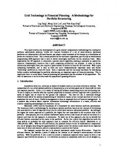
An Information-Theoretic Approach for Clonal Selection Algorithms Vincenzo Cutello, Giuseppe Nicosia, Mario Pavone, Giovanni Stracquadanio Department of Mathematics and Computer Science University of Catania V.le A. Doria 6, I-95125 Catania, Italy {cutello, nicosia, mpavone, stracquadanio}@dmi.unict.it

Abstract. In this research work a large set of the classical numerical functions were taken into account in order to understand both the search capability and the ability to escape from a local optimal of a clonal selection algorithm, called i-CSA. The algorithm was extensively compared against several variants of Differential Evolution (DE) algorithm, and with some typical swarm intelligence algorithms. The obtained results show as i-CSA is effective in terms of accuracy, and it is able to solve large-scale instances of well-known benchmarks. Experimental results also indicate that the algorithm is comparable, and often outperforms, the compared nature-inspired approaches. From the experimental results, it is possible to note that a longer maturation of a B cell, inside the population, assures the achievement of better solutions; the maturation period affects the diversity and the effectiveness of the immune search process on a specific problem instance. To assess the learning capability during the evolution of the algorithm three different relative entropies were used: Kullback-Leibler, R´enyi generalized and Von Neumann divergences. The adopted entropic divergences show a strong correlation between optima discovering, and high relative entropy values. Keywords: Clonal selection algorithms, population-based algorithms, information theory, relative entropy, global numerical optimization.

1

Introduction

Global optimization is the task of finding the set of values that assures the achievement of a global optimum for a given objective function; these problems are typically difficult to solve due to the presence of many local optimal solutions. Since in many realworld applications analytical solutions are not available or cannot be approximated, derivative-free methods are often the only viable alternative. Without loss of generality, the global optimization requires finding a setting x = (x1 , x2 , . . . , xn ) ∈ S, where S ⊆ Rn is a bounded set on Rn , such that the value of n-dimensional objective function f : S → R is minimal. In particular, the goal for global minimization problem is to find a point xmin ∈ S such that f (xmin ) is a global minimum on S, i.e. ∀x ∈ S : f (xmin ) ≤ f (x). The problem of continuous optimization is a difficult task, both because it is difficult to decide when a global (or local) optimum has been reached, and because there could be many local optima that trap the search process. As the problem dimension increases, the number of local optima can grow dramatically.

2

In this paper we present a clonal selection algorithm (CSA), labelled as i-CSA, to tackle global optimization problems as already proposed in [8, 9]. The following numerical minimization problem was taken into account: min(f (x)), Bl ≤ x ≤ Bu , where x = (x1 , x2 , . . . , xn ) ∈ Rn is the variable vector, i.e. the candidate solution; f (x) is the objective function to minimize; Bl = (Bl1 , Bl2 , . . . , Bln ), and Bu = (Bu1 , Bu2 , . . . , Bun ) represent, respectively, the lower and the upper bounds of the variables such that xi ∈ [Bli , Bui ] with i = (1, . . . , n). Together with clonal and hypermutation operators, our CSA incorporates also the aging operator that eliminates the old B cells into the current population, with the aim to generate diversity inside the population, and to avoid getting trapped in a local optima. It is well known that producing a good diversity is a central task on any population-based algorithm. Therefore, increasing or decreasing the allowed time to stay in the population (δ) to any B cell influences the performances and convergence process. In this work, we show that increasing δ in CSA, as already proposed in [8, 9], we are able to improve its performances. Two different function optimization classes were used for our experiments: unimodal and multimodal with many local optima. These classes of functions were used also to understand and analyze the learning capability of the algorithm during the evolution. Such analysis was made studying the learning gained both with respect to initial distribution (i.e. initial population), and the ones based on the information obtained in previous step. Three relative entropies were used in our study to assess the learning capability: Kullback-Leibler, R´enyi generalized and Von Neumann divergences [16, 18, 19]. Looking the learning curves produced by the three entropies is possible to observe a strong correlation between the achievement of optimal solutions and high values of relative entropies.

2

An Optimization Clonal Selection Algorithm

Clonal Selection Algorithm (CSA) is a class of AIS [1–4] inspired by the clonal selection theory, which has been successfully applied in computational optimization and pattern recognition tasks. There are many different clonal selection algorithms in literature, some of them can be found in [20]. In this section, we introduce a variant of the clonal selection algorithm already proposed in [8, 9], including its main features, as cloning, inversely proportional hypermutation and aging operators. i-CSA presents a population of size d, where any candidate solution, i.e. the B cell receptors, is a point of the search space. At the initial step, that is when t = 0, any B cell receptor is randomly generated in the relative domain of the given function: each variable in any B cell receptor is obtained by xi = Bli + β · (Bui − Bli ), where β ∈ [0, 1] is a real random value generated uniformly at random, and Bli and Bui are, respectively, the lower and the upper bounds of the i − th variable. Once it has been (t=0) created the initial population Pd , and has been evaluated the fitness function f (x) for each x receptor, i.e. computed the given function, the immunological operators are applied. The procedure to compute the fitness function has been labelled in the pseudo-code (table 1) as comp fit(∗). Through the cloning operator, a generic immunological algorithm produces individuals with higher affinity (i.e. lower fitness function values for

3

minimization problems), by introducing blind perturbations (by means of a hypermutation operator) and selecting their improved mature progenies. The Cloning opera(clo) tor clones each B cell dup times producing an intermediate population PN c , where N c = d × dup. Since any B cell receptor has a limited life span into the population, like in nature, become an important task, and sometime crucial, to set both the maximum number of generations allowed, and the age of each receptor. As we will see below, the Aging operator is based on the concept of age associated to each element of the population. This information is used in some decisions regarding the individuals. Therefore one question is what age to assign to each clone. In [5], the authors proposed a CSA to tackle the protein structure prediction problem where the same age of the parent has been assigned to the cloned B cell, except when the fitness function of the mutated clone is improved; in this case, the age was fixed to zero. In the CSA proposed for numerical optimization [8, 9], instead, the authors assigned as age of each clone a random value chosen in the range [0, τB ], where τB indicates the maximum number of generations allowed. A mixing of the both approaches is proposed in [11] to tackle static and dynamic optimization tasks. The strategy to set the age of a clone may affect the quality of the search inside the landscape of a given problem. In this work we present a simple variant of CSA proposed in [8, 9] obtained by randomly choosing the age in the range [0, 32 τB ]. According to this strategy, each B cell receptor is guaranteed to live more time into the population than in the previous version. This simple change produces better solutions on unconstrained global optimization problems, as it is possible to note in section 4. Table 1. Pseudo-code of the i-CSA i-CSA (d, dup, ρ, τB , Tmax ) f en := 0; N c := d × dup; (t=0) Pd := init pop(d); (t=0) comp fit(Pd ); f en := f en + d; while (f en < Tmax )do (t) (clo) PN c := Cloning (Pd , dup); (hyp) (clo) PN c := Hypermutation(PN c , ρ); (hyp) comp fit(PN c ); f en := f en + N c; (t) (hyp) (t) (hyp) (P ad , P aN c ) := aging(Pd , PN c , τB ); (t+1) (t) (hyp) Pd := (µ + λ)-selection(P ad , P aN c ); t := t + 1; end while

(clo)

The hypermutation operator acts on the B cell receptor of PN c , and tries to mutate each B cell receptor M times without an explicit usage of a mutation probability. Its feature is that the number of mutations M is determined in inversely proportional way

4

respect fitness values; as the fitness function value increases, the number of mutations performed on it decreases. There are nowadays several different kinds of hypermutation operators [12] and [13]. The number of mutations M is given by the mutation rate: ˆ α = e−ρf (x) , where fˆ(x) is the fitness function value normalized in the range [0, 1]. As described in [8, 9], the perturbation operator for any receptor x randomly chooses a variable xti , with i ∈ {1, . . . , `} (` is the length of B cell receptor, i.e. the problem dimension), and replace it with     (t+1) (t) (t) xi = (1 − β) × xi + β × xrandom , (t)

(t)

where xrandom 6= xi is a randomly chosen variable and β ∈ [0, 1] is a real random number. All the mutation operators apply a toroidal approach to shrink the variable value inside the relative valid region. To normalize the fitness into the range [0, 1], instead to use the optimal value of the given function, we have taken into account the best current fitness value in Pdt , decreased of an user-defined threshold Θ, as proposed in [8, 9]. This strategy is due to making the algorithm as blind as possible, since is not known a priori any additional information concerning the problem. The third immunological operator, aging operator, has the main goal to design an high diversity into the current population, and hence avoid premature convergence. It acts on the two popu(t) (hyp) lations Pd , and PN c , eliminating all old B cells; when a B cell is τB + 1 old it is erased from the current population, independently from its fitness value. The parameter τB indicates the maximum number of generations allowed to each B cell receptor to remain into the population. At each generation, the age of each individual is increased. Only one exception is made for the best receptor; when generating a new population the selection mechanism does not allow the elimination of the best B cell. After the ag(t) (hyp) ing operator is applied, the best survivors from the populations P ad and P aN c are (t+1) selected for the new population Pd , of d B cells. If only d1 < d B cells survived, then (µ + λ)-Selection operator (with µ = d and λ = N c) pick at random d − d1 B cells among those “died” from the set   (hyp) (t) (t) (hyp) (Pd \ P ad ) t (PN c \ P aN c ) . Finally, the evolution cycle ends when the fitness evaluation number (f en) is greater or equal to the allowed maximum number of fitness function evaluations, labelled with Tmax ; f en is a counter that is increased whenever the procedure comp fit(∗) is called. Table 1 summarizes the proposed CSA described above.

3

Kullback-Leibler, R´enyi and von Neumann Entropic Divergences

A study on the learning process of i-CSA during the evolution was made, using three different divergence metrics, as Kullback-Leibler, R´enyi generalized, and Von Neumann divergences. These information were obtained both with respect the initial distribution, and the ones in previous step.

5

Shannon’s entropy [15] is a commonly used measure in information theory and it represents a good measure of randomness or uncertainty, where the entropy of a random variable is defined in terms of its probability distribution. Shannon’s theory, information is represented by a numerically measurable quantity, using a probabilistic model. In this way, the solutions of a given problem can be formulated in terms of the obtained amount of information. Kullback-Leibler divergence (KLd ) [16], also known as Information gain, is one of the most frequently used information-theoretic distance measure, based on two probability distributions of discrete random variable, called relative information, which found many applications in setting important theorems in information theory and statistics. This divergence measures the quantity of information the system discovers during the learning phase with respect to the initial population [6]. (t) We define the B cells distribution function fm as the ratio between the number, t Bm , of B cells at time step t with fitness function value m, and the total number of B cells: Bt Bt (t) = m. fm = Ph m t d m=0 Bm The KLd is formally defined as: (t)

(t) (t0 ) KLd (fm , fm )=

X

fm

(t) fm log

(t )

fm 0

m

! .

The gain is the amount of information the system has already learned during its search

Information Gain 25 f5 f7

f10 20

15

10

5

0 1

2

4

8

16

32

Generations

Fig. 1. Learning of the problem. Kullback-Leibler curves of i-CSA algorithm on the functions f5 , f7 , and f10 . Each curve was obtained over 50 independent runs, with the following parameters: d = 100, dup = 2, τB = 15, ρ = 3.5 and Tmax = 5 × 105 .

process, with respect to the randomly generated initial population P (t=0) (initial distribution). Once the learning process begins the information gain increases monotonically

6

until it reaches a final steady state (see figure 1). This is consistent with the idea of a d maximum Kullback-Leibler principle [17] of the form: dKL ≥ 0. Since the learning dt dKLd process will end when dt = 0, then such maximum principle may be used as termination condition [6, 14]. We are aware that the same metric can be adopted to study the gain of information regarding the spatial arrangement of the solution in the search landscape; in particular, in these terms, when the gain goes to zero it states that the individuals represent the same solution. Figure 1 shows the KLd curves obtained by i-CSA, on the functions f5 , f7 , and f10 of the classical benchmark used for our experiments, and proposed in [7]. In this figure one can see as the algorithm gains quickly amounts of information on the functions f7 and f10 , rather than on f5 , whose KLd is slower; it starts to gain information after generation number 20. This is due because the search space on f5 seems to be more complex than in f7 and f10 , and this behavior is consistent with the obtained experimental results, where i-CSA, and optimization algorithms in general, need a greater number of fitness function evaluations to achieve a good solution. The curves plotted in such figure were obtained with the following experimental protocol: d = 100, dup = 2, τB = 15, ρ = 3.5 and Tmax = 5 × 105 . This experiment was performed over 50 independent runs.

Clonal Selection Algorithm: i-CSA 25

20

300

15

250 200 10

150 100 50

5

0 16

32

64

0 16

32

64

Generations

Fig. 2. Kullback-Leibler curves of i-CSA algorithm on the function f5 . The inset plot shows the standard deviation. Both curves are a zoom into the range [16, 64].

Together with the amount of information learned during the search process, we want to know the uncertainty over the population of i-CSA during all performed runs. Therefore, the standard deviation was also used, which measures the dispersion of a set of data from its mean: more the data are spread apart, higher is the standard deviation. The plot 2 shows the monotonous behavior of the information gain only on function f5 (being one of the most complex), whilst in the inset plot is plotted the standard deviation measure. Both curves are a zoom into the range [16, 64]. The standard deviation

7

increases quickly (the spike in the inset plot) when the algorithm begins to learn information; once the algorithm begins to gain more information, i.e. after 2 − 3 generations from beginning the learning process, the curve of the standard deviation decreases towards zero. The algorithm converges to the best solution in this temporal window. Thus, the highest point of information learned corresponds to the lowest value of uncertainty.

Clonal Selection Algorithm: i-CSA 4e+09

avg fitness best fitness

3.5e+09 3e+09 25

gain entropy

Fitness

2.5e+09 20 2e+09

15 10

1.5e+09

5 1e+09

0 16

32

64

5e+08 0 0

2

4

6

8

10

Generations

Fig. 3. Average fitness versus best fitness of i-CSA on the function f5 , for the first 10 generations. The inset plot shows the entropy and information gain curves. Each curve was obtained over 50 independent runs, with the following parameters: d = 100, dup = 2, τB = 15, ρ = 3.5 and Tmax = 5 × 105 .

In figure 3 we show the average fitness and the best fitness for i-CSA in the first 10 generations, where the algorithm quickly decreases from solutions of the order 109 , until to reach solutions of the order (101 − 1). Also in this figure, the inset plot shows the curves of the information gain, and the entropies. In the last two plots, the best solution found during the experiments is 0.0, whilst the mean of the best solutions is 15.6, with 14.07 as standard deviation. The experiments were obtained using the following parameters: d = 100, dup = 2, τB = 15, ρ = 3.5 and Tmax = 5 × 105 . Since the validity of the metrics is independent from the specific form adopted, we have evaluated the learning capability of i-CSA also with respect two well-known entropic divergences: (1) R´enyi generalized divergence (Rd ) [18], formally defined as ! (t) α X fm 1 (t) (t0 ) log , Rd (fm , fm , α) = (t0 ) α−1 α−1 m f m

with α > 0 and α 6= 1, and (2) Von Neumann divergence (V Nd ) [19], defined as: (t) (t0 ) V Nd (fm , fm )=−

1 X (t) 1 X (t) (t0 ) (t) (fm log fm )− (f log fm ) n m n m m

8 Learning with respect to initial distribution (t0) 30

Von Neumann distribution (VNd) Renyi generalized Kullback-Leibler entropy

25

1.2

20

1 15

VNd

0.8 0.6

10

0.4 0.2

5

0 16

32

64

0

-5 16

32

64

Generations

Fig. 4. Kullback-Leibler entropy, R´enyi generalized divergence, and Von Neumann entropy curves with respect the initial distribution. The inset plot shows the only Von Neumann distribution, zooming in the y-axis.

In figure 4 is showed the comparison among these different learning measures; KLd and Rd have the same monotonous increasing behavior, although Rd starts to learn information some generations before than KLd , which instead reaches in faster way the first peak. As already saw, Rd loses information in the first generations (around 20 generations), whilst in the same generations KLd neither loses information, but nor even is able to learn information. Since the behavior of the V Nd curve is not easy to understand, the inset plot shows only this curve with a zoom in y axis. We have performed the same experiments with the goal to analyze also the learning process with respect the information obtained at the previous time step (t − 1). The figure 5 shows the behaviors of the learning processes of the three entropies used. From this plot, we see as the Rd entropy continues to have a similar behavior to one analyzed respect to the initial distribution, whilst KLd and V Nd once reached the maximum information (the peak), and thus the greater gain, they begin to lose information. Finally, for all figures shown in this section (from figure 2 to figure 5), we have taken into account the only function f5 being one of the most complex function of the test-bed used.

4

Results

In order to understand the search capability of i-CSA inside the landscape, and also its ability to escape from a local optima, we have used the classical benchmark functions proposed in [7]. In particular, making a proper comparisons on the same functions, we have reduced our experiments on the first 13 functions of this benchmark, which belong to two different categories: unimodal and multimodal with many local search. We will indicate all used functions as (f1 , . . . , f13 ), in the same order as proposed in [7]. Nowadays, in literature there are many evolutionary methodologies able to tackle effectively the global numerical function optimization. Among such algorithms, differential

9 Learning with respect (t-1) time step 30

Von Neumann divergence (VNd) Renyi generalized Kullback-Leibler entropy

25

0.9 0.8 0.7 0.6 0.5 0.4 0.3 0.2 0.1 0

20

15

10

5

VNd

16

32

64

0

-5 16

32

64

Generations

Fig. 5. Kullback-Leibler entropy, R´enyi generalized divergence, and Von Neumann entropy curves with respect the previous time step, i.e. at (t − 1) time step. The inset plot shows the only Von Neumann distribution, zooming in the y-axis.

evolution (DE) has shown better performances than other evolutionary algorithms on complex and continuous search space [23, 24]. Therefore, in this section we present the comparisons of i-CSA, not only with its original version, but also with several variants of the DE published in [25, 21]. For simplicity we will use IA to indicate the algorithm proposed in [8, 9]. As first experiment, IA and i-CSA have been compared each other and with one of the best variants of DE, called rand/1/bin. The results are showed in table 2, and for this comparison was used the same experimental protocol adopted in [21, 8]. We pick as reference results for DE, the experiments carried out in [21]. Two different dimensions were used by fixing n ∈ {30, 100}, with a maximum number of fitness function evaluations Tmax = 5 × 105 , and Tmax = 5 × 106 , respectively. For each function we present the mean of the best B cells on all runs, and, in a new line, the standard deviation. As made in [21], all results below 10−25 obtained by IA and rand/1/bin were reported as 0.0; this instead was not considered for i-CSA. From this comparison, it is possible to note that the new variant improves effectively the results, primarily in the function f5 with n = 30, where i-CSA is able to reach the best solution (0.0), where instead the previous variant IA failed. Further, it is clear that the overall performances of i-CSA are comparable on 30 dimension, instead the algorithm outperforms the ones produced by rand/1/bin DE variant on 100 dimension variables ((f3 , f4 , f7 , f10 , f11 ) versus (f5 , f8 , f13 )), which are among the most complex functions. In table 3, IA and i-CSA are compared with 8 DE variants, proposed in [25], where Tmax was fixed to 1.2 × 105 [25, 9]. For each function 100 independent runs were performed, and the variables dimension was fixed to 30. Because in [25], the authors have modified the function f8 to have its minimum at zero (rather than −12569.5), it is not included into the table. Looking the comparison in such table, we can see that the variant of the

10 Table 2. Comparison between IA, i-CSA and rand/1/bin variant The mean of the best individuals on all runs and the standard deviation (in a new line) are presented for all algorithms, and we highlight in boldface the best results, except when the results are the same. The showed results are obtained using n = 30 and n = 100 dimensional search space. IA f1 f2

0.0 0.0 0.0 0.0

i-CSA 30 variables 0.0 0.0 0.0 0.0

f3

0.0 0.0

0.0 0.0

f4

0.0 0.0 12 13.22 0.0 0.0

0.0 0.0 0.0 0.0 0.0 0.0

1.521 × 10−5 2.05 × 10−5 −1.256041 × 10+4

7.48 × 10−6 6.46 × 10−6 −9.05 × 10+3 1.91 × 104

f5 f6 f7 f8 f9 f10 f11 f12 f13

f1 f2

25.912 0.0 0.0 0.0 0.0 0.0 0.0 0.0 0.0 0.0 0.0 0.0 0.0 0.0 0.0

0.0 0.0 0.0 0.0 0.0 0.0 0.0 0.0 0.0 0.0 100 variables 0.0 0.0 0.0 0.0

f3

0.0 0.0

0.0 0.0

f4

6.447 × 10−7 3.338 × 10−6 74.99 38.99 0.0 0.0 1.59 × 10−5 3.61 × 10−5

0.0 0.0 22.116 39.799 0.0 0.0 1.2 × 10−6 1.53 × 10−6

−4.16 × 10+4 2.06 × 10+2 0.0 0.0

−2.727 × 10+4 7.63 × 10−4 0.0 0.0

f10

0.0 0.0

0.0 0.0

f11

0.0 0.0 0.0 0.0 0.0 0.0

0.0 0.0 0.0 0.0 0.0 0.0

f5 f6 f7 f8 f9

f12 f13

DE rand/1/bin [21] 0.0 0.0 0.0 0.0 2.02 × 10−9 8.26 × 10−10 3.85 × 10−8 9.17 × 10−9 0.0 0.0 0.0 0.0 4.939 × 10−3 1.13 × 10−3 −1.256948 × 10+4 2.3 × 10−4 0.0 0.0 −1.19 × 10−15 7.03 × 10−16 0.0 0.0 0.0 0.0 −1.142824 4.45 × 10−8 0.0 0.0 0.0 0.0 5.87 × 10−10 1.83 × 10−10 1.128 × 10−9 1.42 × 10−10 0.0 0.0 0.0 0.0 7.664 × 10−3 6.58 × 10−4 −4.1898 × 10+4 1.06 × 10−3 0.0 0.0 8.023 × 10−15 1.74 × 10−15 5.42 × 10−20 5.42 × 10−20 0.0 0.0 −1.142824 2.74 × 10−8

proposed IA outperform the several DE variants in all functions, except only for the functions f5 and f7 . Recently, immune systems have been related to swarm systems, since many immune algorithms operate in a very similar manner. Thus, we have compared i-CSA with some swarm intelligence algorithms, proposed in [10]: particle swam optimization (PSO); particle swarm inspired evolutionary algorithm (PS-EA), and artificial bee colony. For this kind of experiments we have used the same experimental protocol used in [10]; we consider problems of various dimension ranging in n = {10, 20, 30}; the ter-

11 Table 3. Comparison between IA, i-CSA, and several DE variants. The mean of the best individuals on all runs are presented for all algorithms, and the best results are highlighted in boldface. Results have been averaged over 100 independent runs, using Tmax = 1.2 × 105 , and n = 30 dimensional search space. For i-CSA was fixed d = 100. f1 i-CSA 0.0 IA 0.0 DE rand/1/bin 0.0 DE rand/1/exp 0.0 DE best/1/bin 0.0 DE best/1/exp 407.972 DE current-to-best/1 0.54148 DE current-to-rand/1 0.69966 DE current-to-rand/1/bin 0.0 DE rand/2/dir 0.0

i-CSA IA DE rand/1/bin DE rand/1/exp DE best/1/bin DE best/1/exp DE current-to-best/1 DE current-to-rand/1 DE current-to-rand/1/bin DE rand/2/dir

f5 16.2 11.69 19.578 6.696 30.39087 132621.5 30.984666 31.702063 24.260535 30.654916

Unimodal Functions f2 f3 0.0 0.0 0.0 0.0 0.0 0.02 0.0 0.0 0.0 0.0 3.291 10.6078 4.842 0.471730 3.503 0.903563 0.0 0.000232 0.0 30.112881 Multimodal Functions f9 f10 0.0 0.0 0.0 0.0 0.0 0.0 97.753938 0.080037 0.0 0.0 40.003971 9.3961 98.205432 0.270788 92.263070 0.164786 0.0 0.0 0.0 0.0

f4 f6 f7 0.0 0.0 2.79 × 10−5 0.0 0.0 4.89 × 10−5 1.9521 0.0 0.0 3.7584 0.84 0.0 0.0017 0.0 0.0 1.701872 2737.8458 0.070545 4.2337 1.394 0.0 3.298563 1.767 0.0 0.149514 0.0 0.0 0.044199 0.0 0.0 f11 0.0 0.0 0.001117 0.000075 0.000722 5.9278 0.219391 0.184920 0.0 0.0

f12 0.0 0.0 0.0 0.0 0.0 1293.0262 0.891301 0.464829 0.001007 0.0

f13 0.0 0.0 0.0 0.0 0.000226 2584.85 0.038622 5.169196 0.000114 0.0

mination criterion was fixed to 500, 750, and 1000 generations, respectively. Only five functions were taken into account for these experiments, labelled (g1 , . . . , g5 ), where the first four are included in the same benchmark cited above which corresponding exactly: g1 = f11 , g2 = f9 , g3 = f5 , and g4 = f10 1 . From table 4, it is possible to affirm that i-CSA all swarm system algorithms on all functions, except on the function g5 . The best performances of i-CSA are confirmed also for an increasing problem dimension. Conversely, for the function g5 , PS-EA reaches best solutions respect increasing problem dimension. Finally, the results reported for ABC2 were obtained using a different experimental protocol: the termination criterion was increased to 1000, 1500 and 2000, respectively. Although i-CSA has been tested with a smaller number of generations is possible to notice that the results are comparable, and often outperform ABC2 . This experimental evidence show as i-CSA reaches competitive solutions, near to global optima, in less time than artificial bee colony algorithm.

5

Conclusions

Global numerical optimization has been taken into account to prove the effectiveness of a derivative-free clonal selection algorithm, called i-CSA. The main features of i-CSA can be summarized as: (1) the cloning operator, which explores the neighbourhood of a given solution, (2) the inversely proportional hypermutation operator, that perturbs each 1

For details on these five functions see [10].

12 Table 4. Comparison between i-CSA and several Swarm Intelligence algorithms. For each function is showed the mean and standard deviation (in a new line), obtained on 30 independent runs. The best results have been highlighted in boldface.

GA PSO PS-EA i-CSA ABC1 ABC2

g1

g2

0.050228 0.029523 0.079393 0.033451 0.222366 0.0781 0.0 0.0 0.00087 0.002535

1.3928 0.76319 2.6559 1.3896 0.43404 0.2551 0.0 0.0 0.0 0.0

0.000329 0.00185

0.0 0.0

1.0139 0.026966 PSO 0.030565 0.025419 PS-EA 0.59036 0.2030 i-CSA 0.0 0.0 ABC1 2.01 × 10−8 6.76 × 10−8 ABC2 0.0 0.0 GA

1.2342 0.11045 PSO 0.011151 0.014209 PS-EA 0.8211 0.1394 i-CSA 0.0 0.0 ABC1 2.87 × 10−9 8.45 × 10−10 ABC2 0.0 0.0 GA

g3 g4 g5 10 variables 46.3184 0.59267 1.9519 33.8217 0.22482 1.3044 −13 4.3713 9.8499 × 10 161.87 2.3811 9.6202 × 10−13 144.16 25.303 0.19209 0.32037 29.7964 0.1951 1.6185 0.0 0.0 1.27 × 10−4 0.0 0.0 1.268 × 10−14 0.034072 7.8 × 10−11 1.27 × 10−9 0.045553 1.16 × 10−9 4 × 10−12

0.012522 0.01263 20 variables 6.0309 103.93 1.4537 29.505 12.059 77.382 3.3216 94.901 1.8135 72.452 0.2551 27.3441 0.0 0.0 0.0 0.0 −8 1.45 × 10 0.13614 −8 5.06 × 10 0.132013 0.0 0.014458 0.0 0.010933 30 variables 10.4388 166.283 2.6386 59.5102 32.476 402.54 6.9521 633.65 3.0527 98.407 0.9985 35.5791 0.0 0.0 0.0 0.0 0.033874 0.219626 0.181557 0.152742 0.0 0.020121 0.0 0.021846

4.6 × 10−11 5.4 × 10−11

1.27 × 10−9 4 × 10−12

0.92413 0.22599 1.1778 × 10−6 1.5842 × 10−6 0.32321 0.097353 0.0 0.0 1.6 × 10−11 1.9 × 10−11 0.0 1 × 10−12

7.285 2.9971 543.07 360.22 1.4984 0.84612 237.5652 710.4036 19.83971 45.12342 0.000255 0

1.0989 0.24956 1.4917 × 10−6 1.8612 × 10−6 0.3771 0.098762 0.0 0.0 3 × 10−12 5 × 10−12 0.0 0.0

13.5346 4.9534 990.77 581.14 3.272 1.6185 2766.804 2176.288 146.8568 82.3144 0.000382 1 × 10−12

candidate solution as a function of its fitness function value (inversely proportionally), and (3) the aging operator, that eliminates the oldest candidate solutions from the current population in order to introduce diversity and thus avoiding local minima during the search process. Since any B cell receptor has a limited life span into the population becomes crucial the decision of the age to assign to each B cell receptor. Therefore, the strategy adopted to assign such value to the clones may affect the quality of the search inside the landscape of the given problem and, hence, the capability to escape from a local optima. In this work we present a simple variant of the CSA proposed in [8, 9], which is able to effectively improve its performances allowing a longer maturation of any B cell. A large set of classical numerical functions was taken into account from [7],

13

which is divided into two different categories: unimodal and multimodal (with many local optima) functions. i-CSA was compared with several variants of the DE algorithm, since it has been shown to be effective on many optimization problems. Afterwards, because nowadays immunological systems are considered similar to swarm systems, we have compared i-CSA with state-of-the-art swarm algorithms. The analysis of the results shows that i-CSA is comparable, and often outperforms, all nature-inspired algorithms in terms of accuracy to the accuracy, and effectiveness in solving large-scale instances. By analyzing one of the most difficult function of the benchmark, (f5 ), we characterize the learning capability of i-CSA. The obtained gain has been analyzed both with respect the initial distribution, and the ones obtained in the previous step. For this study, three different entropic metrics were used, as Kullback-Leibler, R´enyi and von Neumann divergences [16, 18, 19]. By the relative curves, is possible to observe a strong correlation between optima (peaks in the search landscape) discovering, and high relative entropy values.

References 1. J. Timmis, A. Hone, T. Stibor, E. Clark: “Theoretical advances in artificial immune systems”, Theoretical Computer Science, vol. 403, no. 1, pp. 11–32, 2008. 2. S. Smith, J. Timmis: “An Immune Network Inspired Evolutionary Algorithm for the Diagnosis of Parkinsons Disease”, Biosystems, vol. 94, no. (1–2), pp. 34–46, 2008. 3. J. Timmis, E. Hart, A. Hone, M. Neal, A. Robins, S. Stepney, A. Tyrrell: “ImmunoEngineering”, in Proc. of the international conference on Biologically Inspired Collaborative Computing (IFIP’09), IEEE Press, vol. 268, pp. 3–17, 2008. 4. D. Dasgupta, F. Ni˜no: “Immunological Computation: Theory and Applications”, CRC Press (in press). 5. V. Cutello, G. Nicosia, M. Pavone, J. Timmis: ”An Immune Algorithm for Protein Structure Prediction on Lattice Models”, IEEE Trans. on Evolutionary Computation, vol. 11, no. 1, pp. 101–117, 2007. 6. V. Cutello, G. Nicosia, M. Pavone: ”An immune algorithm with stochastic aging and kullback entropy for the chromatic number problem”, Journal of Combinatorial Optimization, vol. 14, no. 1, pp. 9-33, 2007. 7. X. Yao, Y. Liu, G. M. Lin: “Evolutionary programming made faster”, IEEE Trans. on Evolutionary Computation, vol. 3, no. 2, pp. 82–102, 1999. 8. V. Cutello, G. Nicosia, M. Pavone, G. Narzisi: “Real Coded Clonal Selection Algorithm for Unconstrained Global Numerical Optimization using a Hybrid Inversely Proportional Hypermutation Operator”, in Proc. of the 21st Annual ACM Symposium on Applied Computing (SAC’06), vol. 2, pp. 950–954, 2006. 9. V. Cutello, N. Krasnogor, G. Nicosia, M. Pavone; “Immune Algorithm versus Differential Evolution: A Comparative Case Study Using High Dimensional Function Optimization”, in Proc. of the International Conference on Adaptive and Natural Computing Algorithms (ICANNGA’07), LNCS, vol. 4431, pp. 93–101, 2007. 10. D. Karaboga, B. Baturk: “A powerful and efficient algorithm for numerical function optimization: artificial bee colony (ABC) algorithm”, Journal of Global Optimization, vol. 39, pp. 459–471, 2007. 11. M. Castrogiovanni, G. Nicosia, R. Rascun´a ”Experimental Analysis of the Aging Operator for Static and Dynamic Optimisation Problems”, in Proc. of the 11th International Conference on Knowledge-Based and Intelligent Information and Engineering Systems (KES’07), LNCS, vol. 4694, pp. 804–811, 2007.

14 12. V. Cutello, G. Nicosia, M. Pavone: “Exploring the capability of immune algorithms: a characterization of hypermutation operators”, in Proc. of the Third International Conference on Artificial Immune Systems (ICARIS’04), LNCS, vol. 3239, pp. 263–276, 2004. 13. V. Cutello, G. Nicosia, M. Pavone: “An Immune Algorithm with Hyper-Macromutations for the Dill’s 2D Hydrophobic-Hydrophilic Model”, in Proc. of Congress on Evolutionary Computation (CEC’04), IEEE Press, vol. 1, pp. 1074–1080, 2004. 14. V. Cutello, G. Nicosia, M. Pavone: “A Hybrid Immune Algorithm with Information Gain for the Graph Coloring Problem”, in Proc. of Genetic and Evolutionary Computation COnference (GECCO’03), LNCS 2723, pp. 171–182, 2003. 15. C. E. Shannon: ”A Mathematical Theory of Communication”, Congress on Evolutionary Computation, Vol. 1, pp. 1074–1080, IEEE Press (2004) Bell System Technical Journal, Vol. 27, pp. 379–423 and 623–656 (1948) 16. S. Kullback S.: ”Statistics and Information Theory”, J. Wiley and Sons, New York (1959) 17. Jaynes E.: ”Probability Theory: The Logic of Science”, Cambridge University Press, 2003. 18. A. R´enyi: ”On measures of information and entropy”, in Proc. of the 4th Berkeley Symposium on Mathematics, Statistics and Probability, pp. 547–561, 1961. 19. A. Kopp, X. Jia, S. Chakravarty: ”Replacing energy by von Neumann entropy in quantum phase transitions”, Annals of Physics, vol. 322, no. 6, pp. 1466–1476, 2007. 20. V. Cutello, G. Narzisi, G. Nicosia, M. Pavone: “Clonal Selection Algorithms: A Comparative Case Study using Effective Mutation Potentials”, in Proc. of the Fourth International Conference on Artificial Immune Systems (ICARIS’05), LNCS, vol. 3627, pp. 13–28, 2005. 21. J. Versterstrøm, R. Thomsen: ”A Comparative Study of Differential Evolution, Particle Swarm Optimization, and Evolutionary Algorithms on Numerical Benchmark Problems”, in Congress on Evolutionary Computing (CEC’04), vol. 1, pp. 1980–1987, 2004. 22. N. Noman, H. Iba: ”Enhancing Differential Evolution Performance with Local Search for High Dimensional Function Optimization”, in Genetic and Evolutionary Computation Conference (GECCO’05), pp. 967–974, 2005. 23. R. Storn, K. V. Price: ”Differential Evolution a Simple and Efficient Heuristic for Global Optimization over Continuous Spaces”, Journal of Global Optimization, vol. 11, no. 4, pp. 341–359, 1997. 24. K. V. Price, M. Storn, J. A. Lampien: ”Differential Evolution: A Practical Approach to Global Optimization”, Springer-Verlag, 2005. 25. E. Mezura–Montes, J. Vel´ azquez–Reyes, C. Coello Coello: ”A Comparative Study of Differential Evolution Variants for Global Optimization”, in Genetic and Evolutionary Computation Conference (GECCO’06), vol. 1, pp. 485–492, 2006.