an instrumental variable approach for identification and estimation ...

Statistica Sinica 24 (2014), 1097-1116 doi:http://dx.doi.org/10.5705/ss.2012.074

AN INSTRUMENTAL VARIABLE APPROACH FOR IDENTIFICATION AND ESTIMATION WITH NONIGNORABLE NONRESPONSE Sheng Wang1 , Jun Shao2,3 and Jae Kwang Kim4 1 Mathematica

Policy Research, 2 East China Normal University, 3 University of Wisconsin and 4 Iowa State University

Abstract: Estimation based on data with nonignorable nonresponse is considered when the joint distribution of the study variable y and covariate x is nonparametric and the nonresponse probability conditional on y and x has a parametric form. The likelihood based on observed data may not be identifiable even when the joint distribution of y and x is parametric. We show that this difficulty can be overcome by utilizing a nonresponse instrument, an auxiliary variable related to y but not related to the nonresponse probability conditional on y and x. Under some conditions we can apply the generalized method of moments (GMM) to obtain estimators of the parameters in the nonresponse probability and the nonparametric joint distribution of y and x. Consistency and asymptotic normality of GMM estimators are established. Simulation results and an application to a data set from the Korean Labor and Income Panel Survey are also presented. Key words and phrases: Consistency and asymptotic normality, generalized method of moments, missing not at random, nonparametric distribution, nonresponse instrument, parametric propensity.

1. Introduction Nonresponse at an appreciable rate exists in many applications. Let y be the value of a study variable subject to nonresponse, δ be the response indicator of y (δ = 1 if y is observed and δ = 0 otherwise), and x be a vector of covariates that are always observed, where x is either deterministic or random with inference conditional on values of x. We assume that an independent sample of size n is obtained with (yi , δi , xi ) being the realized value of (y, δ, x) for sampled unit i = 1, . . . , n, where yi is observed if and only if δi = 1. Let p(y|x) be the conditional density of y given x and p(y) be the marginal density of y. The joint distribution of y and δ given x is determined by p(y|x) and the nonresponse mechanism P (δ = 1|y, x). Nonresponse is said to be ignorable if the nonresponse mechanism is a function of the observed data (Little and Rubin (2002)). Since (y1 , δ1 , x1 ), . . . , (yn , δn , xn ) are independent, ignorable nonresponse in this case

1098

SHENG WANG, JUN SHAO AND JAE KWANG KIM

means that P (δ = 1|y, x) = P (δ = 1|x). For ignorable nonresponse, there is a rich literature on deriving valid estimators of unknown parameters in p(y|x) or p(y). When P (δ = 1|y, x) depends on y that may be missing, which is the focus of this paper, nonresponse is nonignorable and the construction of valid estimators is a challenging problem. Greenlees, Reece, and Zieschang (1982) and Baker and Laird (1988) proposed likelihood methods under some parametric assumptions on both P (δ = 1|y, x) and p(y|x). However, a fully parametric approach is sensitive to the parametric model assumptions. Since the population is not identifiable when both P (δ = 1|y, x) and p(y|x) are nonparametric (Robins and Ritov (1997)), efforts have been made in some cases where one of P (δ = 1|y, x) and p(y|x) is parametric and the other is nonparametric. Tang, Little, and Raghunathan (2003) considered the situation where p(y|x) is parametric but P (δ = 1|y, x) is nonparametric, whereas Qin, Leung, and Shao (2002), Chang and Kott (2008), and Kott and Chang (2010) focused on the case where P (δ = 1|y, x) is parametric but p(y|x) is nonparametric. In many applications, such as survey problems, it is difficult to find a suitable parametric model for p(y|x), but a parametric model for P (δ = 1|y, x) such as the logistic may be reasonable. Although Greenlees, Reece, and Zieschang (1982), Qin, Leung, and Shao (2002), Chang and Kott (2008), and Kott and Chang (2010) proposed some estimation methods, their results rely on the assumption that the observed likelihood is identifiable. Identifiability is necessary for the existence of consistent estimators of parameters (Gelfand and Sahu (1999)). It has been studied in the case of parametric p(y|x) (Chen (2001)); Tang, Little, and Raghunathan (2003)) and some semiparametric p(y|x) (Rotnitzky and Robins (1997)), but it is not well studied in the case of nonparametric p(y|x). In Section 2, we establish a sufficient condition for the identifiability of observed likelihood assuming a parametric model for P (δ = 1|y, x) but without assuming parametric model for p(y|x). The key is to utilize a nonresponse instrument, a component of x that is related to y but not related to the nonresponse conditional on y and other components of x. Without such an auxiliary variable, the observed likelihood may be nonidentifiable even when both p(y|x) and P (δ = 1|y, x) are parametric, as shown in a simple example in Section 2. When the observed likelihood is identifiable, efforts are still needed to develop an estimation method for unknown quantities in p(y|x) or p(y). Qin, Leung, and Shao (2002) applied the empirical likelihood approach, while Kott and Chang (2010) used calibration. In Section 3, we propose the generalized method of moments (GMM) for estimation and establish the consistency and asymptotic normality of the GMM estimators. An advantage of the proposed GMM approach is that the asymptotic covariance matrices of the estimators can be explicitly

IDENTIFICATION AND ESTIMATION WITH NONRESPONSE

1099

derived and their consistent estimators can be easily computed, which is useful for statistical inference such as setting confidence regions. In Section 4, some simulation results are on the finite sample performance of the GMM estimators and the related confidence intervals for the population mean. An application to a data example is also included. Section 5 contains some concluding remarks. Proofs are given in the Appendix. 2. Identifiability Since yi is observed if and only if δi = 1, the observed likelihood is ∏ ∏ ∫ P (δi = 1|yi , xi )p(yi |xi ) [1 − P (δi = 1|y, xi )]p(y|xi )dy, i: δi =1

(2.1)

i: δi =0

where each of P (δ = 1|y, x) and p(y|x) may be parametric or nonparametric. It is identifiable if two different populations do not produce the same observed likelihood. Because the second product in (2.1) involves integrals of the quantities in the first product in (2.1), identifiability comes to whether two different populations give the same P (δ = 1|y, x)p(y|x) for all possible values of (y, x). Even if both P (δ = 1|y, x) and p(y|x) are parametric, identifiability under nonignorable nonresponse is not trivial, as an example indicates. Example 1. Suppose there is no covariate and p(y) is normal with unknown mean µ and variance σ 2 . Let P (δ = 1|y) = [1 + exp(α + βy)]−1 with unknown real-valued α and β. Nonresponse is ignorable if and only if β = 0. Here exp[−(y − µ)2 /2σ 2 ] . P (δ = 1|y)p(y) = √ 2πσ[1 + exp(α + βy)] The observed likelihood is not identifiable if (α, β, µ, σ) and (α′ , β ′ , µ′ , σ ′ ) produce exp[−(y − µ′ )2 /2σ ′2 ] exp[−(y − µ)2 /2σ 2 ] = ′ σ[1 + exp(α + βy)] σ [1 + exp(α′ + β ′ y)]

for all y.

(2.2)

But (2.2) holds if σ = σ ′ , α′ = −α, β ′ = −β, α = (µ′2 − µ2 )/2σ 2 , and β = (µ′ − µ)/σ 2 . Hence, the observed likelihood is not identifiable unless β = β ′ = 0 (ignorable nonresponse). The observed likelihood in Example 1 is identifiable when there is a covariate z such that the conditional distribution of y given z depends on the value of z, and P (δ = 1|y, z) does not depend on z. Theorem 1. The observed likelihood (2.1) is identifiable under the following conditions.

1100


(C1) The covariate x has two components, x = (u, z), such that P (δ = 1|y, x) = P (δ = 1|y, u) = Ψ(αu + βu y),

(2.3)

where αu and βu are unknown parameters not depending on z but may depend on u, Ψ is a known, strictly monotone, and twice differentiable function from R to (0, 1], and, for any given u, there exist two values of z, z1 and z2 (which may depend on u), such that p(y|u, z1 ) ̸= p(y|u, z2 ). (C2) For any given u, p(y|u, z) has a Lebesgue density f (y|u, z) with a monotone likelihood ratio. When a covariate x∗ associated with a study variable y ∗ is measured with error, valid estimators of regression parameters can be obtained by utilizing an instrument z that is correlated with x∗ but independent of y ∗ conditioned on x∗ . In (C1), we decompose the covariate vector x into u and z, such that z is correlated with x∗ = (y, u), a “covariate” associated with the “study variable” y ∗ = δ, and z is independent of y ∗ = δ conditioned on x∗ = (y, u). Unconditionally, z may still be related to δ. Since y is subject to nonresponse, not measurement error, we call z a nonresponse instrument, it helps to identify the observed likelihood so that valid estimators of unknown quantities can be obtained (Section 3). The existence of z1 and z2 such that p(y|u, z1 ) ̸= p(y|u, z2 ) means that z is associated with y even in the presence of u. The nonresponse mechanism in (2.3) has a parametric model. Popular parametric models are the logistic model with Ψ(t) = [1 + exp(t)]−1 , and the probit model with Ψ the distribution function of the standard normal. Here f (y|u, z) in (C2) is nonparametric, since its form is not specified. The monotone likelihood ratio property in (C2) is satisfied for many Lebesgue density families, for example, many one-parameter exponential families, the logistic distribution with location parameter zj , and the uniform distribution on the interval (zj , zj + 1). The following result provides another example in which condition (C2) holds. Corollary 1. Suppose (C1) holds and ∂ log(f (y|u, z))/∂y is a monotone function on the support of f (y|u, z), where f (y|u, z) is given in (C2). The observed likelihood (2.1) is identifiable if (i) f (y|u, z) = f (y − φ) with a parameter φ ∈ R and a Lebesgue density f (which may be unknown), or (ii) f (y|u, z) = φj f (φy) with a parameter φ > 0 and a Lebesgue density f (which may be unknown), and either f (y) = 0 or f (y) = f (−y) for y ≤ 0.


1101

3. Estimation Using the data with nonresponse and a parametric p(y|x), we can estimate parameters by maximizing the observed likelihood (2.1). Here we consider nonparametric p(y|x) and the GMM (Hansen (1982); Hall (2005)) for estimation. The key idea of the GMM is to construct a set of L estimating functions gl (ϑ, y, δ, x),

l = 1, . . . , L,

ϑ ∈ Θ,

where Θ is the parameter space containing the true parameter value θ, L ≥ the dimension of Θ, the gl ’s are non-constant functions with E[gl (θ, y, δ, x)] = 0 for all l, and are not linearly dependent. Let (1 ∑ )T 1∑ g1 (ϑ, yi , δi , xi ), . . . , gL (ϑ, yi , δi , xi ) , ϑ ∈ Θ, G(ϑ) = (3.1) n n i

i

where aT denotes the transpose of the vector a. If L is the same as the dimension ˆ = 0. If L is larger than of Θ, then we may be able to find a θˆ such that G(θ) the dimension of Θ, however, a solution to G(ϑ) = 0 may not exist. A GMM estimator of θ can be obtained using a two-step algorithm. 1. Obtain θˆ(1) by minimizing GT (ϑ)G(ϑ) over ϑ ∈ Θ. ˆ be the inverse matrix of the L × L matrix whose (l, l′ ) element is 2. Let W ∑ n−1 i gl (θˆ(1) , yi , δi , xi )gl′ (θˆ(1) , yi , δi , xi ). The GMM estimator θˆ is obtained ˆ G(ϑ) over ϑ ∈ Θ. by minimizing GT (ϑ)W We first consider the situation where x = (u, z), z = (t, z) has a q-dimensional continuous component t and a discrete component z taking values 1, . . . , J, and u is a continuous p-dimensional covariate. Although the observed likelihood (2.1) is identifiable under (C1) and (C2) αu and βu in (2.3) depend on values of u and, hence, there may be uncountably many parameters for the case of continuous u. We assume therefore a condition to replace (2.3): P (δ = 1|y, x) = P (δ = 1|y, u) = Ψ(α + βy + γuT ),

(3.2)

where Ψ is as in (2.3), and (α, β, γ) is a (p+2)-dimensional unknown parameter not depending on values of x. A similar assumption to (3.2) was made in Qin, Leung, and Shao (2002) and Kott and Chang (2010). To estimate (α, β, γ), the GMM can be applied with the L = p + q + J functions  T  d [δw(ϑ) − 1] g(ϑ, y, δ, x) =  tT [δw(ϑ) − 1]  , (3.3) T u [δw(ϑ) − 1]

1102


where d is the J-dimensional row vector whose lth component is I(z = l), I(A) the indicator function of A, w(ϑ) = [Ψ(ϑ1 + ϑ2 y + ϑ3 uT )]−1 , and ϑ = (ϑ1 , ϑ2 , ϑ3 ). The function g is motivated by the fact that, when θ is the true parameter value, E[g(θ, y, δ, x)] = E {ξ [δw(θ) − 1]} = E (E {ξ [δw(θ) − 1] |y, z, u}) { [ ]} E(δ|y, z, u) =E ξ −1 P (δ = 1|y, z, u) = 0, where ξ = (d, t, u)T . We need q + J ≥ 2. If q = 0, the requirement J ≥ 2 is satisfied if z is not a constant. ˆ given by the two-step Take G as at (3.1) with gl the lth function of g, W ˆ γˆ ) the two-step GMM estimator of θ = (α, β, γ). algorithm, and θˆ = (α ˆ , β, Theorem 2. As n → ∞, the following conclusions hold under (C1) with (2.3) replaced by (3.2), and (C3)−(C4). ˆ such that P (s(θ) ˆ = 0) → 1 and θˆ →p θ as n → ∞, where (i) There exists {θ} T ˆ s(ϑ) = −∂[G (ϑ)W G(ϑ)]/∂ϑ and →p denotes convergence in probability. ˜ satisfying s(θ) ˜ = 0 and θ˜ →p θ, (ii) For any sequence {θ} ( ) √ n(θ˜ − θ) →d N 0, (ΓT Σ−1 Γ)−1 , where →d denotes convergence in distribution, Γ is given in (C4), and Σ is the positive definite matrix with E[gl (θ, y, δ, x)gl′ (θ, y, δ, x)] as its (l, l′ )th element, 1 ≤ l, l′ ≤ p + q + J. ˆ is the (p + q + J) × (p + 2) matrix whose lth row is (iii) If Γ 1 ∑ ∂gl (ϑ, yi , δi , xi ) ˆ n ∂ϑ ϑ=θ i

ˆ is the L × L matrix whose (l, l′ )th element is and Σ 1∑ ˆ ˆ yi , δi , xi ), gl (θ, yi , δi , xi )gl′ (θ, n i

ˆT Σ ˆ −1 Γ ˆ →p ΓT Σ−1 Γ. Γ (C3) The parameter space Θ containing the true value θ is an open subset of Rp+2 , E(∥u∥2 + ∥t∥2 ) < ∞, and there is a neighborhood N of θ such that [ { E δ sup (1+∥t∥2 +∥u∥2 )w2 (ϑ) + (1+|y|+∥u∥1 )(1+∥t∥1 +∥u∥1 )|w′ (ϑ)| ϑ∈N


1103

] } +(1+y 2 +∥u∥2 )(1+∥t∥1 +∥u∥1 )|w′′ (ϑ)| < ∞, where ∥ · ∥ is the L2 -norm, ∥ · ∥1 is the L1 -norm, w(ϑ) = [Ψ(ϑ1 + ϑ2 y + ϑ3 uT )]−1 , and w′ and w′′ are the first and second order derivatives of w(·). (C4) The (p + q + J) × (p + 2) matrix  E[δdT w′ (θ)] E[δydT w′ (θ)] E[δdT uw′ (θ)] Γ =  E[δtT w′ (θ)] E[δytT w′ (θ)] E[δtT uw′ (θ)]  E[δuT w′ (θ)] E[δyuT w′ (θ)] E[δuT uw′ (θ)] 

is of full rank. The asymptotic covariance matrix (ΓT Σ−1 Γ)−1 is much simpler than that of the empirical likelihood estimator in Qin, Leung, and Shao (2002), which enˆ −1 . ˆ −1 Γ) ˆT Σ ables us to obtain an easy-to-compute covariance matrix estimator (Γ Kott and Chang (2010) also derived the asymptotic normality of the calibration estimator and its asymptotic covariance matrix, but they required that y given x follows a linear model. Consider some special cases in which (C3) or (C4) can be simplified. First, consider that x = z is a discrete nonresponse instrument. Then (C4) can be simplified to the condition that there exist at least j1 and j2 in {1, . . . , J} such that E[yw′ (θ)|δ = 1, z = j1 ] E[yw′ (θ)|δ = 1, z = j2 ] = ̸ . (3.4) E[w′ (θ)|δ = 1, z = j1 ] E[w′ (θ)|δ = 1, z = j2 ] This condition can be empirically checked using observed yi ’s and the covariate di ’s. In this case, if Ψ(t) = [1 + exp(t)]−1 is logistic, then (C3) simplifies to E(δy 2 ) < ∞ and E[δ exp({2β ± ϵ}y)] < ∞ for some ϵ > 0. A second special case has z = z discrete and u = u a univariate continuous covariate. The full rank assumption on Γ is the key for the results in Theorem 2 and it is implied by any of the following conditions. (1) J ≥ 3 and the points (aj , bj ), j = 1, . . . , J, are not on the same line, where aj =

E[yw′ (θ)|δ = 1, z = j] E[w′ (θ)|δ = 1, z = j]

and

bj =

E[uw′ (θ)|δ = 1, z = j] . E[w′ (θ)|δ = 1, z = j]

(3.5)

(2) Condition (3.4) holds, E[uw′ (θ)|δ = 1] ̸= 0, and the points (aj , bj ), j = 1, . . ., J +1, are not on the same line, where aJ+1 = E[yuw′ (θ)|δ = 1]/E[uw′ (θ)|δ = 1], bJ+1 = E[u2 w′ (θ)|δ = 1]/E[uw′ (θ)|δ = 1], and aj and bj , j = 1, . . . , J, are given in (3.5).

1104


(3) Condition (3.4) holds, E[uw′ (θ)|δ = 1] = 0, and either E[yuw′ (θ)|δ = 1] = 0 or bj − bj2 E[u2 w′ (θ)|δ = 1] ̸= 1 , ′ E[yuw (θ)|δ = 1] aj1 − aj2 where j1 and j2 are given in (3.4) and aj and bj are given in (3.5). Any of (1)−(3) can be empirically checked using observed data. ˆ γˆ ) is obtained, we can estimate the marginal distribution of Once θˆ = (ˆ α, β, y by the empirical distribution putting mass pi on each observed yi , where pi is ˆ i + γˆ uT ). proportional to δi /Ψ(ˆ α + βy i We consider the estimation of the population mean µ = E(y). Once we have estimators α ˆ , βˆ and γˆ , µ can be estimated by µ ˜1 =

δ i yi 1∑ ˆ n Ψ(ˆ α + βyi + γˆ uTi )

(3.6)

i

or by µ ˜2 =

∑ i

δ i yi ˆ i + γˆ uT ) Ψ(ˆ α + βy i

/∑ i

δi . ˆ i + γˆ uT ) Ψ(ˆ α + βy

(3.7)

i

When the number of functions in (3.3) is more than the number of parameters, we can actually obtain a better estimator of µ using the GMM after adding the function h(µ, ϑ, y, δ, x) = µ − δyw(ϑ), to (3.3). The parameters in this GMM are µ, α, β, and γ, and the number of equations is L = p + q + J + 1. The ˆ and γˆ are the same as those obtained by solving resulting GMM estimators α ˆ , β, R = p + q + J equations, but µ ˆ is different from µ ˜1 in (3.6) or µ ˜2 in (3.7). The difference is due to the weight matrix in the second step of the GMM. Let WR be the optimal weight matrix for the GMM based on the R functions in (3.3). ˆ γˆ ) is the GMM After adding h(µ, ϑ, y, δ, x), we can easily show that (˜ µ1 , α ˆ , β, estimators based on R + 1 equations and the weight matrix [ ] WR 0 ˜ WR+1 = . (3.8) 0 1 ˆ γˆ ) is the GMM The weight matrix in (3.8) is not necessarily optimal. If (ˆ µ, α ˆ , β, estimator obtained using the two-step algorithm with the L = R + 1 functions, then the following result holds and µ ˆ is asymptotically more efficient than µ ˜1 ˜ unless WR+1 in (3.8) is optimal. Corollary 2. Assume the conditions in Theorem 2, E(y 2 ) < ∞, and [ { }] E δ sup y 2 w2 (ϑ) + y 2 |w′ (ϑ)| + |y|3 |w′′ (ϑ)| < ∞. ϑ∈N


1105

ˆ γˆ ) be the GMM estimator obtained using the two-step algorithm after Let (ˆ µ, α ˆ , β, adding h(µ, ϑ, y, δ, x) = µ − δyw(ϑ) to the set of functions in (3.3). Then the ˆ γˆ ), result in Theorem 2 holds with θ and θˆ replaced by (µ, α, β, γ) and (ˆ µ, α ˆ , β, respectively. Consider now the general situation where both z and u may have continuous and discrete components. Let u = (v, s) and z = (t, z), where v and t are continuous and s and z are discrete taking values 1, . . . , K and 1, . . . , J, respectively. Assume (C1) with (2.3) replaced by P (δ = 1|y, x) = Ψ(αs + βs y + γs v T ). For each k = 1, . . . , K, we consider the category defined by s = k and apply the GMM for the estimation of θk = (αk , βk , γk ) using  T  d [δw(ϑ) − 1] g(ϑ, y, δ, x) =  tT [δw(ϑ) − 1]  , v T [δw(ϑ) − 1] where d is defined by (3.3) , w(ϑ) = [Ψ(ϑ1 +ϑ2 y +ϑ3 v T )]−1 , and ϑ = (ϑ1 , ϑ2 , ϑ3 ). Let nk be the number of sample units in the category defined by s = k. The unconditional distribution of y can be estimated by the weighted average of these K empirical distributions with weights proportional to nk . Using these estimated distributions, we can estimate parameters in p(y|x) or p(y). Asymptotic results for these estimators similar to those in Theorem 2 and Corollary 2 can be established. 4. Empirical Results We present some results from a simulation study with normally distributed data. Then we apply the proposed method to a data set from the Korean Labor and Income Panel Survey (KLIPS). Finally, we consider another simulation study using a similar population to the real data set. In the two-step algorithm of GMM for the estimation of α, β, γ, and the overall mean µ = E(y), we used the MATLAB function fminsearch to minimize the objective functions G(ϑ)T G(ϑ) ˆ G(ϑ). In all numerical studies, the initial values for α, β, and γ and G(ϑ)T W were 0, and the initial value of µ was the naive estimate µ ˇ, the sample mean of the observed yi ’s. For the estimation of µ, we compared the proposed GMM estimator µ ˆ (Corollary 2), the naive estimate µ ˇ, the estimators µ ˜1 and µ ˜2 given in ÊL , the estimator of µ based on the empirical (3.6) and (3.7), respectively, and µ likelihood method in Qin, Leung, and Shao (2002). The MATLAB function fsolve was used to solve the empirical likelihood estimation equations.

1106


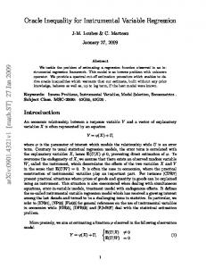
4.1. Simulation from normal populations We considered n = 500 or 2,000 and three populations, each with two sets of parameter values. In the first population, we took x = z as a discrete nonresponse instrument having J = 2 categories with P (z = 1) = 0.4 and P (z = 2) = 0.6. Conditional on z, y ∼ N (20 + 10z, 42 ) with unconditional mean 36. Given the generated data, the nonrespondents were generated according to P (δ = 1|y, z) = [1 + exp(α + βy)]−1 , where (α, β) = (1, −0.05) or (−2.6, 0.05). These values were chosen so that β had different signs. The unconditional nonresponse probability was approximately between 30% and 40%. The second population was similar. The discrete nonresponse instrument z had J = 3 categories with P (z = 1) = 0.3, P (z = 2) = 0.3, and P (z = 3) = 0.4. Given z, y ∼ N (20 + 10z, 42 ), with unconditional mean 41. The nonresponse mechanism is P (δ = 1|y, z) = [1 + exp(α + βy)]−1 , where (α, β) = (1.2, −0.05) or (−2.6, 0.05). In the last population, a continuous covariate u was added, x = (u, z), while z was the same as in the second case. Given z, u ∼ N (100z, 402 ). Given z = 1 and u, y ∼ N (u, 202 ); given z = 2 and u, y ∼ N (1.5u, 202 ); given z = 3 and u, y ∼ N (300 + 0.5u, 202 ). The unconditional mean of y was 300. The nonresponse mechanism was P (δ = 1|y, u, z) = [1 + exp(α + βy + γu)]−1 , where (α, β, γ) = (0.4, −0.002, −0.003) or (−2, 0.002, 0.003). Table 1 reports the following, based on 2,000 simulations: the bias of the ˆ γˆ (for the last case only), µ GMM estimates, α ˆ , β, ˆ, the naive estimate µ ˇ, µ ˜1 ˜2 in (3.7), and the empirical likelihood estimate µ ÊL (Qin, Leung, and in (3.6), µ Shao (2002)); the standard deviation (SD) of GMM estimates, µ ˇ, µ ˜1 , µ ˜2 and µ ÊL ; the standard error (SE) for GMM estimates, the estimated SD using the squared ˆT Σ ˆ −1 Γ) ˆ −1 given in Theorem root of the diagonal elements in the matrix n−1 (Γ 2(iii), and for µ ˇ using the sample standard deviation; the coverage probability (CP) of the approximate 95% confidence intervals [ˆ µ − 1.96SE, µ ˆ + 1.96SE] and [ˇ µ − 1.96SE, µ ˇ + 1.96SE]. The values of parameters and J are also included in Table 1. The simulation results in Table 1 support the asymptotic results for the GMM estimators as well as the consistency of the variance estimators. When there is no covariate u, the GMM estimators work well for J = 2 and J = 3, although performance is generally better when J = 3. The coverage probabilities of the confidence intervals based on µ ˆ are all close to the nominal level 95%. The naive estimator µ ˇ has a positive bias when β < 0 (larger y has smaller nonresponse probability) and has a negative bias when β > 0 (larger y has larger nonresponse probability). Although the bias of µ ˇ may be small compared with the value of µ, it is not small compared with the SD so that it leads to a poor performance of the confidence interval based on µ ˇ. The performance of µ ˜1 , µ ˜2


1107

Table 1. Simulation results for normal populations. n = 2, 000 Parameter J µ α β 2 36 1 -0.05

2 36 -2.6

3 41 1.2

3 41 -2.6

3 300 0.4

3 300 -2

n = 500 2 36 1

2 36 -2.6

3 41 1.2

3 41 -2.6

3 300 0.4

3 300 -2

γ 0

Bias SD SE CP 0.05 0 Bias SD SE CP -0.05 0 Bias SD SE CP 0.05 0 Bias SD SE CP -0.002 -0.003 Bias SD SE CP 0.002 0.003 Bias SD SE CP -0.05

0

Bias SD SE CP 0.05 0 Bias SD SE CP -0.05 0 Bias SD SE CP 0.05 0 Bias SD SE CP -0.002 -0.003 Bias SD SE CP 0.002 0.003 Bias SD SE CP

µ ˆ 0.0054 0.1607 0.1616 94.3% 0.0018 0.1657 0.1622 94.3% -0.0026 0.2207 0.2169 94.8% 0.0025 0.2227 0.2207 94.1% -0.0591 3.4081 3.4389 94.6% -0.2169 3.3770 3.4413 95.2%

µ ˇ 0.6217 0.1646 0.1675 4.8% -0.6115 0.1743 0.1708 4.8% 1.2686 0.2371 0.2417 0.0% -1.5214 0.2539 0.2581 0.0% 26.9383 3.8300 3.8950 0.0% -26.5431 4.1205 4.1872 0.0%

0.0228 0.3189 0.3224 94.2% 0.0025 0.3354 0.3247 94.3% 0.0338 0.4259 0.4324 95.5% -0.0039 0.4382 0.4410 94.7% -0.1934 6.7338 6.8748 95.5% -0.0200 6.8694 6.8721 94.3%

0.6249 0.3429 0.3345 55.4% -0.6166 0.3420 0.3418 4.8% 1.2961 0.4775 0.4818 23.5% -1.5356 0.5138 0.5165 15.1% 26.704 7.4839 7.8109 7.4% -25.710 8.1686 8.3815 12.5%

µ ˜1

Estimate µ ˜2 µ ÊL

α ˆ βˆ -0.0148 3.7/104 0.3671 0.0104 0.3523 0.0100

γ ˆ

-0.0222 4.7/104 0.3908 0.0105 0.3847 0.0103 -0.0210 -0.0055 -0.0052 -0.0063 1.2/104 0.2243 0.2214 0.2208 0.2395 0.0061 0.2426 0.0061 -0.0125 0.0066 0.0025 -0.0321 6.4/104 0.2225 0.2225 0.2210 0.2717 0.0062 0.2564 0.0059 -0.2354 -0.0729 -0.0596 0.0086 5.8/105 -1.5/104 3.4295 3.4091 3.4032 0.1447 0.0018 0.0030 0.1429 0.0018 0.0029 -0.3235 -0.2149 -0.2213 -0.0057 3.3/105 5.8/105 3.2911 3.4084 3.2961 0.1626 0.0016 0.0024 0.1442 0.0015 0.0024

-0.0452 0.0011 0.7003 0.0198 0.7110 0.0201 -0.0517 0.0012 0.7858 0.0209 0.7744 0.0207 -0.0400 0.0195 0.0218 0.0198 -6.7/104 0.4368 0.4258 0.4240 0.4914 0.0123 0.4916 0.0123 -0.0642 0.0015 -0.0087 -0.0701 0.0014 0.4485 0.4448 0.4380 0.5683 0.0130 0.5374 0.0120 -0.8013 -0.2047 -0.1449 0.0192 2.9/104 -7.6/104 6.7379 6.7295 6.7148 0.2988 0.0035 0.0059 0.2900 0.0036 0.0060 -0.3105 0.2197 0.0541 -0.0065 -5.8/105 1.4/104 6.7988 7.0382 6.7577 0.3376 0.0032 0.0049 0.2959 0.0031 0.0049

1108


and µ ÊL are similar to that of µ ˆ in terms of both bias and standard deviation, indicating that the weight matrix in (3.8) is nearly optimal. When the number of equations is equal to the number of parameters (J = 2 case), they are all identical. 4.2. Estimates for the KLIPS data We applied the proposed method to a data set from the KLIPS. A brief description of this survey can be found at http://www.kli.re.kr/klips/en/about/introduce.jsp. The data set consists of n = 2, 506 regular wage earners. The variable of interest, y, is the monthly income in 2006. Covariates associated with y are gender, age group, level of education, and the monthly income in 2005. The variable y has about 35% missing values while all covariate values are observed. To apply the proposed method, we first used the income in 2005 as a continuous covariate u and the age, gender, and education levels as a discrete nonresponse instrument z. Thus we assumed that these covariates are related to y and u but they are not related to the nonresponse once y and u are given. Unconditionally, these covariates may still be related to the nonresponse. We took age 0. Let y ∗ = (α − α′ )/(β ′ − β). Since α + βy ∗ = α′ + β ′ y ∗ , we have K(y ∗ ) = 0. For any y > y ∗ , α + βy = α + βy ∗ + β(y − y ∗ ) < α + βy ∗ + β ′ (y − y ∗ ) = α′ + β ′ y.

(A.3)

Since Ψ is strictly decreasing, it follows from (A.3) that Ψ(α + βy) > Ψ(α′ + β ′ y) and, therefore, K(y) = [Ψ(α+βy)/Ψ(α′ + β ′ y)]− 1 > 0. Similarly, when y < y ∗ , K(y) < 0. This proves that K(y) has a single change of sign. Step II. We prove that, if β ̸= β ′ and if the first integral in (A.2) is 0, then the second integral is not 0. Let X be a random variable having f1 or f2 as its probability density and let Ej denote the expectation when X has density fj . We show that if E1 [K(X)] = 0, then E2 [K(X)] ̸= 0, where K is the function defined in Step I with β ̸= β ′ . Let K(x) < 0 if x < x0 and K(x) > 0 if x > x0 , and put f2 (x) c = sup . x 0, c = f2 (x0 )/f1 (x0 ) < ∞. When f1 (x0 ) = 0, because E1 [K(X)] = 0, there exists x1 such that x1 > x0 and f1 (x1 ) > 0, which implies that c ≤ f2 (x1 )/f1 (x1 ) < ∞. Thus, c < ∞. Write ∫ ∫ ∫ E2 (K(X)) = K(x)f2 (x)dx = K(x)f2 (x)dx + K(x)f2 (x)dx, A

B

where A = {x : f1 (x) = 0, f2 (x) > 0} and B = {x : f1 (x) > 0, f2 (x) > 0} ∪ {x : f1 (x) > 0, f2 (x) = 0}. If x ∈ A, then f2 (x)/f 1 (x) = ∞ and, therefore, x > x0 . ∫ This shows that K(x) > 0 for x ∈ A and A K(x)f2 (x) ≥ 0. Then ∫ E2 [K(X)] ≥ K(x)f2 (x)dx ∫B ∫ = K(x)f2 (x)dx + K(x)f2 (x)dx B1 B2 ∫ ∫ f2 (x) f2 (x) f1 (x)dx + K(x) f1 (x)dx = K(x) f (x) f 1 1 (x) B2 B1 ∫ ∫ ≥ cK(x)f1 (x)dx + cK(x)f1 (x)dx B1

B2

1114


= cE1 [K(X)] = 0, where B1 = {x : x ∈ B, x < x0 }, B2 = {x : x ∈ B, x > x0 }, and the last inequality follows from the definition of c and the fact that K(x) < 0 for x ∈ B1 and K(x) > 0 for x ∈ B2 . ∫ If A has a positive Lebesgue measure, then A K(x)f2 (x)dx > 0 and, hence, E2 [K(X)] > 0. If A has Lebesgue measure 0, then the support sets of f1 and f2 are subsets of B. If E2 [K(X)] = 0, then f2 (x) = cf1 (x) a.e. on B. Then, c = 1 because f1 and f2 are densities. This contradicts (C1). Therefore, we have E2 [K(X)] > 0. Thus, (A.2) implies β = β ′ and reduces to ∫ [ ∫ [ ] ] Ψ(α + βy) Ψ(α + βy) − 1 f (y)dy = − 1 f2 (y)dy = 0, 1 Ψ(α′ + βy) Ψ(α′ + βy) which implies α = α′ since Ψ(x) is a strictly monotone function. These results and (A.1) imply that f1 = f1′ and f2 = f2′ , which shows identifiability. Proof of Theorem 2. ˜ →p W , where W is a positive definite matrix. First, we (i) Suppose that W prove that there exists θ¯ such that, as n → ∞, ¯ = 0) → 1 P (˜ s(θ)

and

θ¯ →p θ,

(A.4)

˜ G(ϑ)]/∂ϑ. Since Γ is of full rank and W is positive where s˜(ϑ) = −∂[GT (ϑ)W definite, ΓT W Γ is positive definite. Therefore, there exists a matrix A such that A2 = 2ΓT W Γ. ˜ G(ϑ). To prove (A.4), it suffices to prove that, for Define Q(ϑ) = GT (ϑ)W any ϵ > 0, there exists c > 0 such that, for sufficiently large n, P {Q(θ) − Q(ϑ) < 0 for all ϑ ∈ Bn (c)} ≥ 1 − ϵ, (A.5) √ √ where Bn (c) = {ϑ : ∥A(ϑ − θ)∥ = c/ n} and ∥A∥ = trace(AT A) for a vector or matrix A. When n is large enough, Bn (c) is inside the parameter space Θ and Bn (c) shrinks to θ as n → ∞. By Taylor’s expansion, there exists θ∗ between θ and ϑ such that 1 Q(θ) − Q(ϑ) = (ϑ − θ)T s˜(θ) + (ϑ − θ)T ∇˜ s(θ∗ )(ϑ − θ) 2 c c2 T −1 λ A ∇˜ s(θ∗ )A−1 λ, = √ λT A−1 s˜(θ) + 2n n √ where ∇˜ s(ϑ) = ∂˜ s(ϑ)/∂ϑ, λ = nA(ϑ − θ)/c, and ∥λ∥ = 1 for ϑ ∈ Bn (c). Using ˜ →p W , the proof of Theorem 2.6 in Newey and Mcfadden (1994) and (C3), W


1115

the fact that every component in G(ϑ), ∂G(ϑ)/∂ϑ, and ∂ 2 G(ϑ)/∂ϑ∂ϑT is an average over independent and identically distributed samples, we obtain that sup ∥∇˜ s(ϑ) − ψ(ϑ)∥ →p 0, ϑ∈N

where ψ(ϑ) = −∂ 2 {E[GT (ϑ)]W E[G(ϑ)]}/∂ϑ∂ϑT . Since ψ(θ) = −2ΓT W Γ, ∥∇˜ s(θ∗ ) − (−2ΓT W Γ)∥ ≤ ∥∇˜ s(θ∗ ) − ψ(θ∗ )∥ + ∥ψ(θ∗ ) − (−2ΓT W Γ)∥ ≤ sup ∥∇˜ s(ϑ) − ψ(ϑ)∥ + ∥ψ(θ∗ ) − ψ(θ)∥ ϑ∈N

→p 0 by the continuity of ψ at θ. Hence A−1 ∇˜ s(θ∗ )A−1 →p −I2×2 . Then, { } 1 c2 T −1 √ Q(θ) − Q(ϑ) = cλ A n˜ s(θ) − [1 + op (1)] n 2 { } c2 1 T −1 √ n˜ s(θ)] − [1 + op (1)] ≤ c max[λ A λ n 2 { } 2 √ c 1 −1 c∥A n˜ s(θ)∥ − [1 + op (1)] . (A.6) = n 2 √ ˜ √nG(θ). Under Let ∇G(ϑ) = ∂G(ϑ)/∂ϑ. Then A−1 n˜ s(θ) = −2A−1 ∇G(θ)W √ (C3), ∇G(θ) →p Γ by the Law of Large Numbers and nG(θ) →d N (0, Σ) by ˜ →p W , the Central Limit Theorem. By the fact that W √ A−1 n˜ s(θ) →d N (0, 4A−1 ΓT W ΣW ΓA−1 ). √ Therefore, there exists a c such that P (∥A−1 n˜ s(θ)∥ < c/4) ≥ 1 − ϵ. Now √ −1 ∥A n˜ s(θ)∥ < c/4 and (A.6) imply Q(θ) − Q(ϑ) < 0 for all ϑ ∈ Bn (c). Hence, result (A.5) follows and the proof of (A.4) is complete. ˜ = IL×L , we obtain that θˆ(1) →p θ, which, combined with By (A.4) with W ˆ →p Σ−1 . Then the result in (i) follows from (A.4) with (C3), implies that W ˜ ˆ W = W and W = Σ−1 , where Σ−1 is a positive definite matrix. ˜ = (ii) By Taylor’s expansion, there exists a θ∗ between θ and θ˜ such that G(θ) ∗ ˜ G(θ) + ∇G(θ )(θ − θ), which implies that ˜ TW ˜ = [∇G(θ)] ˜ TW ˜ TW ˆ G(θ) ˆ G(θ) + [∇G(θ)] ˆ ∇G(θ∗ )(θ˜ − θ). [∇G(θ)] ˜ TW ˜ = s(θ) ˜ = 0, we obtain that ˆ G(θ) Since −2[∇G(θ)] √ √ ˜ TW ˜ TW ˆ ∇G(θ∗ )}−1 [∇G(θ)] ˆ nG(θ). n(θ˜ − θ) = −{[∇G(θ)] θ∗

Σ−1

(A.7)

˜ →p Γ, ˆ →p Since θ˜ →p θ, we have →p θ which, together with W and ∇G(θ) imply that ˜ TW ˜ TW ˆ ∇G(θ∗ )}−1 [∇G(θ)] ˆ →p (ΓT Σ−1 Γ)−1 ΓT Σ−1 . {[∇G(θ)] (A.8) √ By the Central Limit Theorem, nG(θ) →d N (0, Σ) which, combined with (A.7) and (A.8), proves part (ii) of the theorem.

1116


References Baker, S. and Laird, N. M. (1988). Regression analysis with categorical data subject to nonignorable nonresponse. J. Amer. Statist. Assoc. 83, 62-69. Chang, T. and Kott, P. S. (2008). Using calibration weighting to adjust for nonresponse under a plausible model. Biometrika 95, 557-571. Chen, S. X., Leung, D. H. and Qin, J. (2008). Improving semiparametric estimation by using surrogate data. J. Roy. Statist. Soc. Ser. B 70, 803-823. Chen, K. (2001). Parametric models for response-biased sampling. J. Roy. Statist. Soc. Ser. B 63, 775-789. Gelfand, A. E. and Sahu, S. K. (1999). Identifiability, improper priors, and Gibbs sampling for generalized linear models. J. Amer. Statist. Assoc. 94, 247-253. Greenlees, J. S., Reece, W. S. and Zieschang, K. D. (1982). Imputation of missing values when the probability of response depends on the variable being imputed. J. Amer. Statist. Assoc. 77, 251-261. Hall, A. R. (2005). Generalized Method of Moments. Oxford University Press, New York. Hansen, L. (1982). Large sample properties of generalized method of moments estimators. Econometrica 50, 1029-1054. Kott, P. S. and Chang, T. (2010). Using calibration weighting to adjust for nonignorable unit nonresponse. J. Amer. Statist. Assoc. 105, 1265-1275. Little, R. J. A. and Rubin, D. B. (2002). Statistical Analysis with Missing Data. Second edition. Wiley, New York. Nevo, A. (2003). Using weights to adjust for sample selection when auxiliary information is available. J. Business and Economic Statistics 21, 43-52. Newey, W. and Mcfadden, D. (1994). Large Sample Estimation and Hypothesis Testing. Springer, New York. Qin, J., Leung, D. and Shao, J. (2002). Estimation with survey data under non-ignorable nonresponse or informative sampling. J. Amer. Statist. Assoc. 97, 193-200. Robins, J. M. and Ritov, Y. (1997). Toward a curse of dimensionality appropriate (CODA) asymptotic theory for semi-parametric models. Statistics in Medicine 16, 285-319. Rotnitzky, A. and Robins, J. M. (1997). Analysis of semi-parametric regression models with non-ignorable nonresponse. Statist. Medicine 16, 81-102. Tang, G., Little, R. J. A. and Raghunathan, T. E. (2003). Analysis of multivariate missing data with nonignorable nonresponse. Biometrka 90, 747-764. Mathematica Policy Research, Princeton, NJ 08540, U.S.A. E-mail: [email protected] School of Finance and Statistics, East China Normal University, Shanghai 200241, China. Department of Statistics, University of Wisconsin-Madison, Madison, WI 53706, U.S.A. E-mail: [email protected] Department of Statistics, Iowa State University, 1208 Snedecor Hall, Iowa State University, Ames, IA 50011, USA. E-mail: [email protected] (Received March 2012; accepted July 2013)