Department of Electrical Engineering ... pin placement, and which is solved by drawing an analogy between the .... information regarding graph theory and Steiner tree be found in the book by Winter 8]. .... the integer programming formulation gives an optimal layout solution, ..... to nd its route. .... 24] S. Sahni and A. Bhatt.
An Integer Programming Approach to Placement and Routing in Circuit Layout � Ratnesh Kumar Wai Kit Leong Robert J. Heath Department of Electrical Engineering University of Kentucky Lexington, KY 40506-0046 Abstract
A circuit layout problem requires determining the component pin placement and routing of interconnections for a given circuit schematic on a single or multilayer printed circuit board. In this paper, an integer programming based approach is introduced to solve the layout problem which performs placement and routing simultaneously. Since an integer programming problem is computationally intractable, a heuristic method to solve the placement and routing separately has been developed by utilizing the integer programming formulation. By applying a xed routing scheme that connects components by direct line segments, the layout problem is transformed into a quadratic cost optimization problem in which the only decision variable is the pin placement, and which is solved by drawing an analogy between the quadratic cost term and the power dissipation term in a purely resistive network. Partitioning is then used to assign components to locations on a grid. Once the placement is determined, routing of the interconnections is the only decision variable, which is performed using a new algorithm called virtual grid routing that allows multiple wires to share common grids. Keywords: Printed circuit board, placement, routing, integer programming, Steiner tree
This research was partially supported by the Center for Robotics and Manufacturing Systems, University of Kentucky, and in part by the National Science Foundation under the Grant NSF-ECS-9409712. �
1
1 Introduction Given a circuit schematic, its printed circuit board (PCB) layout requires placement of component pins and routing of pin interconnections on single or multi-layered rectilinear graph representing a PCB. Circuit components include IC chips, resistors, capacitors, etc. The inputs to the problem are the pin distribution of components, and the net list, which describes the interconnections between the pins. The output of the layout problem is an assignment of vertex locations to the pins, and an assignment of edges to the interconnections. Refer to the papers by Soukup [28] and by Shahookar-Mazumdar [27] which survey the related problem of VLSI layout. The layout problem optimizes the cost criteria measured as the total wire length, while ensuring routability. This problem is computationally intractable, i.e., it is NP-complete [20]. Therefore in practice, heuristic methods are employed to solve it. One of these methods is divide-and-conquer, which divides the problem into smaller subproblems, which are then solved individually, either optimally or near-optimally. For the layout problem, the most common way of doing this is to perform component placement under a xed routing scheme, followed by the routing of the interconnections under the xed placement of components determined in the previous step. We present an integer programming formulation to solve the layout problem which performs placement and routing simultaneously. This demonstrates that the layout problem is an instance of the linear integer programming problem. Since an integer programming problem is computationally intractable, a heuristic method to solve the placement and routing separately has been developed by utilizing the integer programming formulation. By applying a xed routing scheme that connects components by direct line segments, the layout problem is transformed into a quadratic cost optimization problem in which the only decision variable is the pin placement, and which is solved by drawing an analogy between the quadratic cost term and the power dissipation term in a purely resistive network. Partitioning is then used to assign components to locations on a grid. Once the placement is determined, routing of the interconnections is the only decision variable, which is performed using a new algorithm called virtual grid routing that allows multiple wires to share common grids. We have implemented our placement and routing algorithms, and the results for a test circuit used by PROTEL for demonstration of their layout CAD tool has been included below. The rest of the paper is organized as follows: The next section introduces the notions for de ning the layout problem. Section 3 obtains the linear integer programming formulation. Sections 4 and 5 study the heuristic placement and routing. The simulation results are given in Section 6, and Section 7 concludes the work presented here.
2 Notation and Preliminaries In this section we introduce the notation used for the mathematical description of the layout problem. The following speci cation of the problem is given: (i) a set of components, 2
(ii) a set of pins for each component, (iii) a net list connecting various pins, and (iv) a rectilinear layout graph. We are required to develop a layout algorithm to place all of the components and route all interconnections on the layout graph so that the total wire length is minimized. Table 1 lists the variables used for de ning the layout problem. Variable What it represents C component list ci component i P pin list pj pin j N net list Nk net k nkl source-sink pair l of net k V vertices located on rectilinear graph vm vertex m [m] index set for vertices neighboring to vm
Table 1: Variables used for de ning the layout problem Let C = fc1; � � � ; ci; � � � ; cI g be the set of components, and P = fp1; � � � ; pj ; � � � ; pJ g be the set of pins of all the components. The pins in this set are listed in an order consistent with the ordering of the component listing in set C , i.e., in P all pins of components ci are listed after those of component ci , whenever i > i0. For simplicity of presentation of integer programming formulation, we assume each component has only two pins. However, as discussed below, the layout formulation can be generalized to deal with components having more than two pins. With this assumption, we have J = 2I . Let P1 � P denote the set of the rst pins of the component, i.e., P1 = fp1; p3; � � � ; p2I ?1 g. We assume that the layout graph is a connected, non-directed rectilinear graph with vertex set V = fv1; � � � ; vm; � � � ; vM g as shown in Figure 1(a). Each vertex can be occupied by a single pin, and each edge can contain only a single interconnection wire. Each vertex vm with the exception those on the boundary has four adjacent vertices. So there are four edges incident on each non-boundary vertex vm. Let [m] be the index set of four possible neighboring p vertices p of a a vertex vm, then for a non-boundary vertex [m] = fm + 1; m ? 1; m + M; m ? M g. Let N be the collection of mutually disjoint sets of net lists: N = SKk=1 Nk , where Nk � P is the kth net list, and it de nes the pins that needs to be connected together. The pins in net Nk must be connected using a Steiner tree so as to minimize the wire length. Then the problem consists of nding a connected Steiner tree subgraph of G for each net Nk whose vertices are occupied by the pins in net Nk , and whose edges connect the vertices by a common wire. Refer to Figure 2. The placement problem refers to determining the vertices of the Steiner trees, and the routing problem refers to determining their edges. Detailed 0
3
1/2
1
2
3
4
M 1/2
1
1/2
M+1
2
3
4
M
1/2
M +1 1/2
2M+1
1/2
M
M-M 1/2
M-M
M-1
M
(a)
(b)
Figure 1: Numbering scheme for the grid points and the grids information regarding graph theory and Steiner tree be found in the book by Winter [8]. We determine the edges of the Steiner trees by using the network ow technique. In the network ow technique for the Steiner tree computation of a net, any pin of the net can be chosen as a source pin, whereas the other pins are chosen as the sink pins. Flows of a unit common source
(a)
(b)
Figure 2: Steiner tree and its source-sink pair nets sharing a common source value start from the common source pin and terminate at distinct sink pins. Refer to Figure 2. The ow path determined by the network ow techniques determines the corresponding Steiner tree. Each of the sink pins is grouped with the common source pinSto form a sourcesink pair net. Let nkl denote the lth source-sink pair net of net Nk : Nk = jlN=1kj nkl , where for a net Nk , each nkl consists of a common source and a distinct sink pin. The network ow 4
method described here can be found in the book by Magnanti [20].
3 Linear Integer Programming Formulation In this section, the integer programming formulation of the layout problem is described in detail. The following table lists the variables used. Variable range Cj;lk -1/0/1 xj;m 0/1 ym;m 0/1 l;k zm;m 0/1 0
0
What it represents source/sink status of pin pj in source-sink pair net nkl assignment status of pin pj to vertex vm connectivity status of edge between vertex vm and its neighbor vm
ow status from vertex vm to vm for source-sink pair net nkl
0
0
Table 2: Variables used for integer programming formulation For each net Nk , a matrix [Cj;lk ]2I �jNkj 2 f?1; 0; 1gk�2I �jNk j is used to hold the source/sink information of pin pj in the source-sink pair net nkl . Cj;lk = 1 if and only if pin pj is a source pin in the source-sink pair of net nkl ; ?1 if and only if it is a sink of that net; and 0 if it is neither a source nor a sink of that net. This source/sink matrix for each net is the main input to our mathematical formulation of the layout problem. We de ne xj;m 2 f0; 1g2I �R to be a binary decision variable to denote the presence of pin pj at vertex vm. Let ym;m 2 f0; 1gM �M be a binary decision variable to denote the presence l;k 2 f0; 1gjNk j�K to of an edge connecting vertices vm and vm . Furthermore, we de ned zm;m M �M be an auxiliary ow variable, which is either zero or one, and represents ow between vertices vm and vm for the source-sink pair net nkl . The constraints for the integer programming formulation are listed below: A1: Each pin must occupy a vertex, i.e., 0
0
0
0
M X
m=1
xj;m = 1; 8j � 2I
A2: Each vertex can have not more than one pin, i.e., 2I X
j =1
xj;m � 1; 8m � M
A3: The second pin of a component must occupy a vertex adjacent to the vertex occupied by the rst pin of the component, i.e., X xj+1;m = xj;m; 8j 2 P1; m � M m 2[m]
0
0
5
Components with more than two pins will impose additional similar constraints for the placement of the rest of the pins. A4: This constraint is a ow balance equation which represents that the net ow corresponding to the source-sink pair net nkl at vertex vm should add up to (i) either 1 if vm is occupied by a source pin of the source-sink pair net nkl , (ii) ?1 if vm is occupied by a sink pin of the source-sink pair net nkl , (iii) and 0, otherwise, i.e., X
l;k ? z l;k ) = (zm;m m ;m
m 2[m] 0
0
0
2I h X Ck
j;l xj;m
j =1
i
; 8k � K; l � jNk j; m � M
l;k is one A5, A6: There is an edge between vm and vm if and only if the ow variable zm;m 0
for some source-sink pair net, i.e.,
0
l;k ; 8l � jN j; k � K; m � M; m0 2 [m]; ym;m � zm;m k 0
0
ym;m � zml;k;m; 8l � jNk j; k � K; m � M; m0 2 [m] 0
0
The complete integer programming formulation looks like: 3
2
X X min 4 21 ym;m 5 m�M m 2[m] 0
0
subject to A1. A2. A3.
M X m=1 2I X j =1
xj;m = 1; 8j � 2I
xj;m � 1; 8m � M
X
m 2[m] 0
A4.
X
0
l;k ? z l;k ) = (zm;m m ;m
m 2[m] 0
A5. A6.
xj+1;m = xj;m; 8j 2 P1; m � M 0
0
l;k ; ym;m � zm;m ym;m � zml;k;m; 0
0
0
0
2I h X Ck
j =1
i
j;l xj;m ; 8k � K; l � jNk j; m � M
8l � jNk j; k � K; m � M; m0 2 [m] 8l � jNk j; k � K; m � M; m0 2 [m]
The cost function counts the number of edges used. The factor 12 in front of the cost function is used to take care of the duplication in counting. Clearly, a solution to the layout problem as formulated above exists if and only if the circuit-graph is planar. Otherwise, one should rst compute the planar sub-graphs of the circuit graph and then use the above formulation to layout each planar sub-graph on di�erent planes or layers. 6
Also, the above formulation shows that the layout problem is an instance of the linear integer programming problem, and can be solved using any commercially available integer programming solver such as GAMS (General Algebraic Modeling System) [1]. An instance of the integer programming problem is known to be computationally intractable. So, although the integer programming formulation gives an optimal layout solution, heuristic techniques are used to obtain sub-optimal layout solutions. The next two sections describe our heuristic placement and routing algorithms.
4 Quadratic Formulation for Placement In the previous section, the integer programming formulation solves the layout problem by determining the placement location for every component and routing for each interconnection such that the total wire length is minimized. In order to consider the placement problem alone, the routing is xed using a predetermined routing strategy. This xed routing scheme does not use Steiner tree pattern of routing, but instead connects each source-sink pair net by the direct line segment connecting them. This approach ignores the routability issue, and only uses the estimated wire length to determine the component placement, which is obtained by adding the squared Eucledian distances between vertices of each source-sink pair nets. The xed routing scheme transforms the integer programming formulation of the layout problem into a quadratic formulation of only the placement problem. In order to solve the the quadratic formulation, we rst obtain a relative placement of components by allowing placement locations to occupy any point on a plane instead of only the points on the grid. To solve the relative placement problem, we utilize the resistive network method proposed by Cheng and Kuh [4], which views the quadratic cost function as the power dissipation term in a purely resistive network. It is well known that the problem of power dissipation minimization in a purely resistive network is equivalent to obtaining the current distribution in the network using Kircho�'s laws. So the quadratic optimization problem reduces to solving a set of linear simultaneous equations. Table 3 lists the additional notation introduced in this section. Variable What it represents Cj;j connectivity count between pins pj and pj dm;m squared Eucledian distance between vertices vm and vm 0
0
0
0
Table 3: Additional notations used for heuristic placement
4.1 Relative Placement
Since the placement and orientation of a component is uniquely determined by any two of its pins, we continue to assume that each component ci in C has only two pins. We will 7
relax this assumption when we perform the routing of interconnections. Let Cj;j denote the connectivity count between pins pj and pj . Each pin represents an aggregation of all pins in one half of a component; so Cj;j is the total number of connections between component halves containing pins pj and pj respectively. Recall that the two pins of component ci are p2i?1 and p2i. In order to ensure that two pins of each component are placed next to each other, for each i we set the connectivity count C2i?1;2i to be a su�ciently large number. Let dm;m denote the squared Eucledian distance between vertices vm and vm of the rectilinear layout graph. Then a wire of estimated length dm;m is present if and only if vertices vm and vm are occupied by pins sharing common nets, i.e., if and only if there exist j and j 0 such that the assignment variables xj;m and xj ;m as well as the connectivity count Cj;j are non-zero. So under the xed routing scheme the integer programming formulation reduces to the following quadratic formulation, in which the only decision variable is the pin assignment variable: 0
0
0
0
0
0
0
0
0
0
0
3
2
X X X X dm;m xj;mxj ;m Cj;j 5 min 4 21 j �2I j �2I m�M m �M 0
0
subject to A1. A2.
0
M X m=1 J X j =1
0
0
0
xj;m = 1; 8j � 2I
xj;m � 1; 8m � M
Note that the constraint A3 which ensures that the second pin of a component is placed adjacent to its rst pin is trivially satis ed due to the assignment of a su�ciently large connectivity count for each such pin pair. So we have not included constraint A3 in the above formulation. Also note that the edge assignment variable ym;m does not appear in the above formulation since it is xed and is no more a decision variable. Consequently, the constraints A4-A6 which refer to this decision variable also do not appear in the above formulation. Since Cj;j is a constant for summations with respect to m and m0, the quadratic cost function can be rewritten as: 3 2 1 X X C 4 X X d x x 5: (1) 2 j�2I j �2I j;j m�M m �M m;m j;m j ;m 0
0
0
0
0
0
0
0
From constraint A1, for any xed j and j 0, xj;m is non-zero for exactly one m, and xj ;m is non-zero for exactly one m0. So the term dm;m xj;m xj ;m is non-zero for exactly one m; m0 pair. Hence the sum X X (2) dm;m xj;mxj ;m 0
0
0
0
m�M m �M
0
0
0
0
0
in (1) equals the distance between those vertices where pins pj and pj get assigned. Letting (xj ; yj ) and (xj ; yj ) denote the coordinates of the assignment location of pin pj and pj , the 0
0
0
0
8
sum in (2) is the single distance term: [(xj ? yj )2 + (xj ? yj )2]; which is the squared Eucledian distance between grid coordinates (xj ; yj ) and (xj ; yj ). So the quadratic cost function of (1) becomes: I;2I h 1 2X 2i 2 C j;j (xj ? xj ) + (yj ? yj ) : 2 j;j This quadratic cost function can be rewritten as: " #" # i B 0 h X T T X Y 0 B Y ; where X2I �1 is the vector with j th entry xj , Y2I �1 is the vector with j th entry yj ; B = D ? C is a 2I � 2I symmetric matrix with C = [Cj;j ]2I �2I being the connectivity matrix, and D2I �2I is a diagonal matrix whose j th diagonal entry Dj;j is equal to P2j I Cj;j . The following proof shows that the above two cost functions are identical. I;2I h 1 2X 2 + (y ? y )2i C ) ( x ? x j j 2 j;j j;j j j 2X I;2I h i = 21 Cj;j x2j ? 2xj xj + x2j + yj2 ? 2yj yj + yj2 j;j 2X I;2I 2 I;2I 2X I;2I X 1 1 2 2 = 2 Cj;j xj + 2 Cj;j xj ? xj xj Cj;j + j;j j;j j;j 2 I;2I 2 I; 2 I 2 I; 2 I 1 X C y2 + 1 X C y2 ? X 2 j;j j;j j 2 j;j j;j j j;j yj yj Cj;j 2X I;2I 2I 2I 2I X 2I X X X = 21 x2j Cj;j + 21 x2j Cj;j ? xj xj Cj;j + j j j;j j j 2 I;2I 2I X 2I 2I 2I X X X 1X 1 2 2 y 2 j j j Cj;j + 2 j yj j Cj;j ? j;j yj yj Cj;j 0
0
0
0
0
0
0
0
0
0
0
0
0
0
0
0
0
0
0
0
0
0
0
0
0
0
0
0
0
0
0
0
0
0
0
0
0
0
0
0
0
0
0
0
0
0
0
0
0
0
0
0
0
Since P2j I x2j P2j I Cj;j = P2j I x2j P2j I Cj;j and P2j I yj2 P2j I Cj;j = P2j I yj2 P2j I Cj;j (just interchange the role of j and j 0 in the right side of the equalities and use the symmetry of Cj;j matrix), the above can be simpli ed to: 0
0
0
0
0
0
0
0
0
0
0
2I 2I X X x2 C j
j
=
j
0
2 2I X 4 x2j Dj;j
j
j;j
0
?
?
2X I;2I
j;j 2X I;2I j;j
xj xj Cj;j +
0
3
2I 2I X X y2 C
j 2 2I X
j
j
0
j;j
xj xj Cj;j 5 + 4 yj2Dj;j ? 0
0
0
0
0
j
9
0
?
2X I;2I j;j
2X I;2I j;j
yj yj Cj;j 0
0
3
yj yj Cj;j 5 0
0
0
0
= X T (D ? C )X + Y T (D ? C )Y = X T BX + Y T"BY #" # h i B 0 X T T = X Y 0 B Y :
Note that we have already incorporated constraint A1 which requires that each pin must have a unique placement location in obtaining the above formulation. The second constraint A2 which requires that each placement location must contain at most one pin can be relaxed since in order to only obtain a relative placement we are allowing the pins to be placed anywhere on the plane representing the layout area, and it is unlikely that two or more pins will get assigned to exactly the same point on the plane. Generally, electrical circuits have input and output connectors. These connections normally supply the power and necessary analog and digital signals to the circuit, and provide the output signals for the users. Locations of such connector components on the PCB are often xed by PCB designers. The remaining components such as IC chips, resistors, etc., are movable; and we are only required to nd their placement locations. The objective is to nd the placement of movable components so as to minimize the above quadratic cost. Since we are only interested in relative placement of components we relax the requirement that the components should be placed on grid points, and instead we allow them to be placed at all points on a plane. Mathematically this amounts to expanding the feasible domain of the decision variables from a discrete set to a continuous one, and is a standard approach for dealing with integer programming problems. We describe the resistive network approach for optimizing the quadratic formulation, which reduces the problem to solving linear equations using a resistive network analogy. In a purely resistive network, the power dissipation is given by V T ZV , where V is the vector representing the node voltages and Z is the symmetrical admittance " # matrix. Thus, from B 0 the electric network analogy, in the quadratic formulation 0 B can be view as the admittance matrix of a 4I -terminal passive resistive network, and X and Y can be viewed as the vectors of applied voltages to the network. The presence of xed pins is equivalent to having some xed voltage sources at the corresponding nodes in the resistive network. Suppose there are R movable pins and (2I ? R) xed pins. Then in the electrical analogy model shown in Figure 3, 2R nodes are oating and their voltage are denoted by a 2R-vector V1. The remaining (4I ? 2R) nodes are connected to xed voltage sources denoted by a (4I ? 2R)-vector V2 . Since the current is entering the resistive network only through the sources, the application of Kircho�'s current law yields the following equations: 0 = Z11V1 + Z12V2 (3) i = Z21V1 + Z22V2; (4) where Z11, Z12 = Z21, and Z22 are the appropriate sub-matrices of the admittance matrix Z , and i is the current from the voltage sources. From Equation (3), we can obtain: V1 = ?Z11?1Z12V2; (5) 10
2R+1 1 2R+2
2 . . .
Linear passive resistive network
. . . 4I
2R
+ -
+ -
+ -
Figure 3: 4I -terminal resistive network with 2R oating terminals and others connected to voltage sources which gives the solution for the 2R oating terminal voltages in terms of the (4I ? 2R) xed terminal voltages. It is well known that current and voltage distributions obtained by applying Kircho�'s laws minimize the power dissipation in the network. So a solution to the quadratic cost optimization can be obtained by considering the set of linear equations analogous to that given by Equation (5). In order to apply this to the placement problem separate the locations for the movable and the xed components and rewrite: h
XT Y T
i
"
B 0 0 B
#"
2
B11 i6 Y2T 664 B0 21 0
#
X = h XT Y T XT 1 1 2 Y
B12 0 B22 0
0 B11 0 B21
0 B12 0 B22
X1 3 76 Y 7 76 1 7 7; 76 5 4 X2 5 Y2 32
where subscript 1 (respectively, 2) refers to the coordinates of movable (respectively, xed) components. So the equivalents of Equations (3) and (4) are: "
0 = B011 B0 11 "
#"
#
"
X1 + B12 0 0 B12 Y1 #
#"
#"
X2 Y2
#
#"
"
#
X2 ; X1 + B22 0 i = B021 B0 Y2 0 B22 Y1 21 where B11; B12; B21; B22 are sub-matrices of B of appropriate sizes. This yields the following equation for the locations of the movable components in terms of those of the xed components: # #" # " # " " X2 : X1 = ? B11 0 ?1 B12 0 Y 0 B 0 B Y 1
12
11
2
This placement result gives a solution that minimizes the estimated wire length under the xed routing strategy. However, the constraint to place pins at grid points is ignored. Since 11
components occupy a nite area, they may overlap when we place them at the placement locations we have determined. In the next section, we introduce a partitioning method to overcome the overlapping issue and to assign the components to appropriate locations on a grids.
4.2 Partitioning
Partitioning is needed to assign components to locations on rectilinear grid points using their relative placement locations. Once we determine the coordinates of both pins of each component ci, we can calculate the angle of the rst pin away from the second pin to determine the component orientation. Four possible types of orientation are allowed as shown on Figure 4. Apart from determining the orientation for each component, we also calculate the central coordinate (xci; yic) for every component ci. These central coordinates of the components are used as inputs to our partitioning method. orientation # 1
orientation # 3 pin J/2
pin 2 pin 1 pin 2
pin 2
pin 1 pin J
pin 1 pin 2
pin (J/2)+1
pin 1 pin 1
pin J
pin (J/2)+1
pin 1
pin J
pin (J/2)+1
pin J/2
pin J/2
pin 2
pin 2
pin 1
pin 2
orientation # 2
orientation # 4 pin 2 pin J/2
pin J
pin (J/2)+1
pin 1
Figure 4: Pin orientations and the corresponding component orientations As shown in Figure 5, we introduce a vertical cut line to partition the PCB layout area into two. The location of the cut line is determined so that the total number of pins on each side is approximately equal. We sort the components from left to right and count the number of pins encountered until roughly half of the total pin number is reached. The cut line is then made. The original layout area is divided into two sub-layout areas, which have almost equal number of pins, but the number of components may di�er. The layout area is partitioned alternately in the horizontal and vertical directions until each sub-layout area contains only one component (refer to Figure 5). The result of the partition and the orientation is then used to assign the actual pin locations on a rectilinear grid.
12
x
x
x
x
x
x
x
x
x
x
(a)
x
x
x
(b)
(c)
(e)
(f)
x
x x
(d)
Figure 5: (a) Using coordinates of pins determine the orientation and central coordinate of each components; (b) Use central coordinates as inputs for partitioning; (c) A vertical line partitions the layout area into two sub-layout areas; (d) Further partition of the sub-layout areas; (e) After partitioning, each component has its own grid location; (f) Actual pins are placed on the grid points based on the orientation and placement information
5 Virtual Grid Routing The nal phase of the layout problem is the routing of interconnections on the rectilinear grid. Since the placement phase ignores the routability issue, achieving the largest possible routability of nets is of concern for the routing phase. Reasons such as net ordering and insu�cient routing space [30] are known to a�ect routability even if a placement is routable. The example shown in Figure 6 illustrates these problems. In Figure 6(a), net 1 has been routed, but net 2 has been blocked. If net 2 is routed before routing net 1, the circuit becomes routable as shown in Figure 6(b). Therefore, the order in Figure 6(c) shows that insu�cient routing space can cause net 1 to be blocked even when net 2 is routed rst. One of the solutions for achieving good routability is to detect already routed nets which cause blockage and perform their \rip-up" and \reroute". Dees-Karger and Dees-Smith [6, 5] describe some key strategies on deciding which existing nets should be ripped up and how their routes should be modi ed in order to avoid con icts. Another way is to allow more than one wire to occupy each grid, as shown on Figure 6(d). This new grid routing environment is called virtual grid routing and is described in detail below. It uses the minimum spanning tree to connect the pins on the same net. It is known that the wire length resulting from a minimum spanning tree routing pattern is at worst 50% longer than the optimum wire length resulting from the Steiner tree routing pattern. The reason for the sub-optimal routing is of 13
net1 net2
net2 net1
(a)
net1 net2
net2 net1
net1 net2
net2 net1
net1 net2
(c)
(b)
net2 net1
(d)
Figure 6: Net ordering and insu�cient routing space a�ect routability; later can be avoided by virtual grid routing course the computational complexity issue since the minimum spanning tree computation is polynomial in nature, whereas the Steiner tree computation is an NP-complete problem. Our algorithm uses a modi cation of Lee's algorithm [18] for the minimum spanning tree computation. It is based on propagating a \wave" from one grid to another. At each step of the wave propagation, the grids on the wave front are extended by one further step. Each grid stores a trace back code, so that the origin of the wave source can be traced back after the destination is found. Table 4 lists the additional notation used for routing. Variable What it represents G grid list of the rectilinear layout graph gm grid m [m] index set for grids neighboring to gm W wiring order using net size and MST routing wj wire j
Table 4: Notations used for heuristic routing Let G = fg1; � � � ; gm; � � � ; gM g denote the grid list determined by the actual pin locations (refer to Figure 1(b)). Each grid gm with the exception of the boundary grids p has four p neighbors, whose indices are denoted by [m] = fm + 1; m ? 1; m + M; m ? M g. Note that each grid is a square area, the center of which is occupied by a pin. We route all nets except the power (VCC) and ground (GND) nets, which we assume are routed separately on di�erent layers. In order to determine the routing order, the nets are ordered from the largest to the smallest: all interconnections of a net are routed prior to those of any smaller one. Within a certain net, a minimum spanning tree based routing is used to determine the routing order of the various interconnections. In other words, the shortest source sink pair net is routed rst; and any given step, the pin that is nearest to the spanning sub-tree thus far routed is chosen for wiring to its nearest neighbor on the spanning sub-tree. The corresponding wiring order is listed in the list: W = fw1; � � � ; wj ; : : :; wJ g. 14
We call each grid a virtual grid since we allow multiple wires to pass through a common grid. This avoids blockage of nets caused by insu�cient routing space and thus improves routability. Also, it simpli es the computational complexity of routing by representing routing spaces spanning several grids as a single aggregated grid. There are six allowed directional patterns of wire routes, denoted fNE; SE; SW; NW; NS; EW g, where NE is the north-east direction, SE is the south-east direction, etc., (Figure 7). In order to avoid wire crossing,
(a)
(b)
(c)
(d)
(e)
(f)
Figure 7: Wire direction patterns: NW, NE, SW, SE, EW, and NS north-south and east-west wire paths are required not to share a grid, which is the requirement. Each wire path in a grid has a certain wire pattern and a net number associated with it so that it can be identi ed to which net it belongs. Each grid has six admissible direction patterns, and accordingly contains a set of direction pointers specifying the directions in which wires can be routed. These direction pointers are dynamically modi ed as the wires get routed on each grid to keep track of the allowable directions. Refer to Figure 8 for an illustration. The following algorithm outlines the
(a)
(b)
(c)
(d)
Figure 8: Dashed lines indicate wires that have already been routed, solid lines with arrows indicate allowable wiring directions proposed virtual grid routing technique: 1. Initialize by (i) marking each grid in G as \unsearched", (ii) de ning an empty list Lm for each grid gm , and (iii) de ning a list L0 containing a single grid gm at which the source of the initial wire in list W is located. 2. Determine if a neighboring grid gm of gm is admissible. gm is admissible for routing if there is no overlap with the existing wires of other nets when a wire from gm to gm is added. 0
0
0
15
3. If the neighboring grid gm is admissible for routing, then record the predecessor gm of gm in its list Lm . 4. If grid gm is occupied by a pin of the same net, or if there is an overlap with a wire of the same net when a wire from gm to gm is routed, then the wire is routable; trace the wire route to its origin by using the predecessor grid lists Lm's, and store the wire route. Skip to step 10. 5. If grid gm is marked \unsearched", append it to the list L0. 6. Repeat step 2 for each neighboring grid of gm. 7. Delete grid gm from list L0, and mark it \searched". 8. Repeat step 2 for each grid in list L0. 9. If L0 is empty, then the wire is unroutable. 10. Delete the wire from list W . If W is nonempty, go back to step 1; else stop. In the above algorithm if a certain wire is unroutable, another layer or vias can be used to nd its route. 0
0
0
0
0
0
6 Simulation Results A sample circuit with 36 components and 88 nets is obtained from the demo version of a commercial layout CAD tool called Protel's Printed Circuit Board Layout Tool for Windows. Table 5 gives the distribution of pins in components and nets: pins in components 2 4 8 14 16 28 40
pins in nets 2 3 4 5 6 7 11 30 53
components 19 1 1 3 3 4 4 TOTAL : 36
nets 49 10 3 12 1 10 1 1 1 TOTAL : 88
Table 5: Distribution of pins in components and nets 16
The heuristic algorithms described above have been programmed in ANSI C, and the results of the relative placement and partitioning of the sample circuit are displayed using MATLAB. Figure 9 shows the result of relative placement. Figure 10 shows the enlargement Terminal Coordinates of ALL Components (Initial Placement) 300
200
100
Y-axis
0
-100
-200
-300
-400
-500 -250
-200
-150
-100
-50
0 X-axis
50
100
150
200
250
Figure 9: Relative placement: `x' represents location of xed pins, `o' represents location of movable pins of the placement area occupied by the movable pins. Terminal Coordinates of Movable Components 120
110
Y-axis
100
90
80
70
60 105
110
115
120
125
130 X-axis
135
140
145
150
155
Figure 10: Enlargement of the placement area of movable pins Figure 11 depicts the central coordinates of the movable components. Next partitioning is used to assign the component locations on the grids, the result of which is shown in Figure 12. 17
Center Coordinate of Movable Components 160
150
140
Y-axis
130
120
110
100
90 105
110
115
120
125
130 X-axis
135
140
145
150
155
Figure 11: Central coordinates of movable components
Partition Phase 160
150
140
Y-axis
130
120
110
100
90 105
110
115
120
125
130 X-axis
135
140
145
150
155
Figure 12: Partitioning of the placement area
18
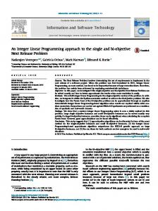
Figure 13 depicts the actual grid assignment of the components. As can be seen, the partitioning phase does not yield a compact placement of componenets (lot of empty space appears within the placement area) and further improvment can be done. 52 44 22
19
17
36
38
40 48
35 20
31 32
23
41
24
18 45
30
37
21 16
28
29
15
12 11
25
38
14
34 27
39
13 43
46
Figure 13: Grid assignment of components Separarte layers are used for routing the nets consisting of the VCC (power) and GND (ground). The routing of the nets other than VCC and GND is shown in Figure 14, which is generated in NeXTSTEP V3.3 using Objective C.
7 Conclusion We have presented an integer programming based approach for the layout problem that performs simultaneous placement and routing. Although the integer programming formulation is speci c to the PCB layout problem, it can also be applied for placement and routing of VLSI circuits by incorporating the appropriate VLSI physical design constraints. Since an integer programming problem is computationally intractable, a heuristic method to solve the placement and routing seperately has been developed that utilizes the integer programming formulation. By applying a xed routing scheme that connects components by direct line segments, the layout problem is transformed into a quadratic problem in which the only decision variable is the component pin placement. Partitioning is then used to 19
52
44
22
23
17
41
19
36
38
40
18 28 35
11
37
45
31
20
48
34 32
43
24
30
12
21
16
38
40
13
46
39 29
Figure 14: Routing of nets excluding VCC and GND nets assign components to locations on a grid. Once the placement is determined, routing of the interconnections is the only decision variable. We have proposes a virtual grid routing technique that avoids the problem of insu�cient routing spaces. We have used estimated wire length under a xed routing for determining placement. Other methods which do not depend on estimation of wire lengths should be investigated and compared with our approach. Our placement algorithm is very e�cient as it only requires solving a set of linear simultaneous equation, however, the resulting component placement after partitioning is not very compact; enough vacant space is present throughout the layout area. Further reserach is needed to improve the compactness of placement. Finally, the algorithm implementation of the virtual grid routing needs further development to make it more e�cient.
References [1] D. Kendrick A. Brooke and A. Meeraus. GAMS A User Guide. The Scienti c Press, South San Francisco, CA, 1988. [2] S. Chang. The generation of minimal trees with a steiner topology. J. ACM, 19(4):699{ 711, October 1972. [3] N. P. Chen. New algorithm for steiner tree on graph. Proceedings of the International Symposium on Circuit and Systems, pages 1217{1219, 1983. [4] C. Cheng and E. Kuh. Module placement based on resistive network. Transaction On Computer Aided Design, (3):218{225, July 1984. 20
[5] W. A. Dees and P. G. Karger. Automated rip-up and reroute techniques. Proceedings of the 19th Design Automation Conference, pages 432{439, 1982. [6] W. A. Dees and R. R. Smith. Performance of interconnection rip-up and reroute strategies. Proceedings of the 18th Design Automation Conference, pages 381{390, 1981. [7] W. E. Donath. Complexity theory and design automation. Proceedings of the 17th Design Automation Conference, pages 412{419, 1980. [8] D. S. Richards F. K. Hwang and P. Winter. The Steiner Tree Problem. Elsevier Science, Amsterdam, Netherlands, 1992. [9] S. Goto. An e�cient algorithm for the two-dimensional placement problem in electrical circuit layout. IEEE Transac. Circuits Syst., pages 12{18, January 1981. [10] S. Goto and E. S. Kuh. An approach to the two-dimensional problem in circuit layout. IEEE Transac. Circuits Syst., pages 208{214, July 1976. [11] K. M. Hall. An r-dimensional quadratic placement algorithm. Manage Science, pages 219{229, November 1970. [12] M. Hanan and J. M. Kurtzberg. A review of placement and quadratic assignment problems. SIAM Review, pages 324{342, April 1972. [13] W. Heyns and W. Sansen. A line expansion algorithm for the general routing with a guaranteed solution. Proceedings of the 17th Design Automation Conference, pages 243{249, 1980. [14] D. Hightower. A solution to the line routing problem on the continuous plane. Proceedings of the Design Automation Conference, pages 1{24, 1969. [15] F. K. Hwang. An o(n log n) algorithm for suboptimal retilinear steiner trees. IEEE Transac. Circuit Syst., pages 75{77, January 1979. [16] B. W. Kerninghan and S. Lin. An e�cient heuristic procedure for partitioning graphs. Bell Systems Tech. J., pages 291{308, 1970. [17] J. Kruskal. On the shortest spanning subtree of a graph and the traveling salesman problem. Proceedings of the American Mathematical Society, 7(1):48{50, 1956. [18] C. Y. Lee. An algorithm for path connections and its application. IRE Trans. Electron. Comput., pages 346{365, September 1961. [19] F. T. Leighton. Complexity issues in VLSI. MIT Press, Cambridge, MA, 1983. [20] Thomas Lengauer. Combinatorial algorithms for integrated circuit layout. WileyTeubner, Chichester, England, 1990. 21
[21] C. Miura M. Mogaki and H. Terai. Algorithm for block placement with size optimization technique by the linear programming approach. Proceedings IEEE International Conference on Computer Aided Design, pages 80{83, 1987. [22] E. Kuh R. Tsay and C. Hsu. Module placement for large chips based on sparse linear equations. International J. Circuit Theory Appl., 16:411{423, 1988. [23] C. D. Gelatt S. Kirkpatrick and M. P. Vecchi. Optimization by simulated annealing. Science, pages 671{680, May 1983. [24] S. Sahni and A. Bhatt. The complexity of design automation problem. Proceedings of the 17th Design Automation Conference, pages 402{411, 1980. [25] D. G. Schweikert. A two-dimensional placement algorithm for the layout of electrical circuit. Proceedings of the 14th Design Automation Conference, pages 408{416, 1976. [26] L. Sha and T. Blank. Atlas: A technique for layout using analytic shapes. Proceedings of the 23th Design Automation Conference, pages 84{87, 1987. [27] K. Shahookar and P. Mazumder. Vlsi cell placement techniques. ACM Computing Surveys, 23(2):143{220, June 1991. [28] J. Soukup. Circuit layout. Proceedings of the IEEE, 69:21{44, October 1981. [29] P. Suaris and G. Kedem. Quadrisection: A new approach to standard cell layout. Proceedings of the IEEE International Conference on Computer Aided Design, pages 474{477, 1987. [30] C. C. Tong and C. L. Wu. A recursive router with 100 Proceedings of the Design Automation Conference, pages 1202{1205, 1991.
22