An Integrated Approach to Locality Conscious Processor Allocation ...

An Integrated Approach to Locality Conscious Processor Allocation and Scheduling of Mixed Parallel Applications

N. V YDYANATHAN , S. K RISHNAMOORTHY, G. S ABIN , U. C ATALYUREK , T. K URC , P. S ADAYAPPAN AND J. S ALTZ

Technical Report OSU-CISRC-2/08-TR04

An Integrated Approach to Locality Conscious Processor Allocation and Scheduling of Mixed Parallel Applications∗ Naga Vydyanathan† , Sriram Krishnamoorthy† , Gerald Sabin† , Umit Catalyurek‡ , Tahsin Kurc‡ , Ponnuswamy Sadayappan† , and Joel Saltz‡ † Dept. of Computer Science and Engineering, ‡ Dept. of Biomedical Informatics The Ohio State University

Abstract Complex parallel applications can often be modeled as directed acyclic graphs of coarse-grained application-tasks with dependences. These applications exhibit both task- and data-parallelism, and combining these two (also called mixed-parallelism), has been shown to be an effective model for their execution. In this paper, we present an algorithm to compute the appropriate mix of task- and dataparallelism required to minimize the parallel completion time (makespan) of these applications. In other words, our algorithm determines the set of tasks that should be run concurrently and the number of processors to be allocated to each task. The processor allocation and scheduling decisions are made in an integrated manner and are based on several factors such as the structure of the task-graph, the runtime estimates and scalability characteristics of the tasks and the inter-task data communication volumes. A locality conscious scheduling strategy is used to improve inter-task data reuse. Evaluation through simulations and actual executions of task graphs derived from real applications as well as synthetic graphs shows that our algorithm consistently generates schedules with lower makespan as compared to CPR and CPA, two previously proposed scheduling algorithms. Our algorithm also produces schedules that have lower makespan than pure task- and data-parallel schedules. For task graphs with known optimal schedules or lower bounds on the makespan, our algorithm generates schedules that are closer to the optima than other scheduling approaches.

1

Introduction

Parallel computing has proven to be a powerful tool for meeting the growing computational requirements of existing and emerging scientific and engineering applications [20, 27]. To optimally exploit the computing capabilities of current massively parallel systems, it is crucial to design algorithms for efficient scheduling of parallel applications on these architectures. A large body of research has addressed this scheduling problem by modeling the parallel application as a directed acyclic graph of sequential ∗

This research was supported in part by the National Science Foundation under Grants #CCF-0342615 and #CNS0403342.

1

Time

Time

T1

T4 T2

T3

T3

T4

T2 T4

T1 P1

(a)

T2

T3 T1

..

P32 Processors

(b)

P1 ..

P16 ..

P32 Processors

(c)

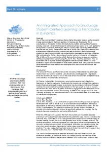
Figure 1. (a) A sample task graph, (b) A pure data-parallel schedule, (c) A mixed-parallel schedule.

tasks with dependences, where a task represents an atomic operation in the application [21]. However, as applications grow in their computational complexity, these task graphs could scale to millions of vertices, making their scheduling intractable. An alternative higher level of abstraction is to view the parallel application as a collection of coarse-grained parallel tasks with data dependences. This model of representation is also known as a macro data-flow graph [30]. Parallel applications represented as macro data-flow graphs can benefit from two forms of parallelism: task- and data-parallelism. Task-parallelism is the concurrent execution of independent tasks of the application on the same or different data elements. Data-parallelism is the parallel execution of a single task on data distributed over multiple processors. For example, in the task graph shown in Figure 1(a), executing tasks T 2 and T 3 concurrently denotes task-parallelism, while executing any of the four tasks on more than one processor denotes data-parallelism. In a pure task-parallel schedule, each task is assigned to a single processor and multiple tasks are executed concurrently as long as precedence constraints are not violated and there are sufficient number of processors in the system. In a pure data-parallel schedule, the tasks are run in a sequence on all available processors. However, a pure task- or a pure data-parallel schedule may not be the optimal execution paradigm for many applications due to the following reasons. Task-parallelism in many applications is often limited by precedence constraints. The sub-linear speedups achieved with increasing number of processors leads to poor performance of pure data-parallel schedules. In fact, several researchers have shown that a combination of both, called mixed parallelism, yields better speedups [8, 30, 15]. In mixedparallel execution, each parallel task in the application is allocated a subset of the processors and several such tasks are executed concurrently. The number of processors allocated to a parallel task denotes its degree of data-parallelism. The number of parallel tasks that are executed concurrently signifies the degree of task-parallelism. The benefit of mixing task- and data-parallelism is illustrated in Figure 1. Consider that the tasks T 2 and T 3 in Figure 1(a) are identical and that their parallel speedup saturates at 16 processors, i.e allocating more than 16 processors does not yield any significant reduction in the task’s execution times. Let their execution time on 16 processors be t time units. A pure data-parallel schedule on 32 processors is illustrated in Figure 1(b) where all four tasks are run on all 32 processors in a sequence. An alternative mixed-parallel schedule is shown in Figure 1(c), where tasks T 2 and T 3 are run concurrently on 16 2

processors each. The concurrent execution of tasks T 2 and T 3 exploits the task-parallelism, while running T 2 and T 3 on 16 processors and T 1 and T 4 on 32 processors exploits the data-parallelism. It is easy to note that this mixed-parallel schedule has a makespan that is lower than the data-parallel schedule by t time units. In this paper, we propose an approach for computing the appropriate mix of task- and data-parallelism needed to minimize the parallel completion time or makespan of applications modeled as macro dataflow graphs. Given the runtime estimates of the tasks, their speedup functions and the inter-task data communication volumes, our algorithm computes the best processor allocation to tasks and the schedule in an integrated manner. To increase inter-task data reuse, we use a locality conscious backfill scheduling scheme. This scheme tries to schedule tasks to the same or overlapping processor groups as their predecessors, whenever possible, to maximize data reuse. Backfill scheduling tries to pack tasks as tight as possible and hence helps in improving the effective processor utilization by minimizing idle time slots. Our algorithm also uses a bounded look-ahead mechanism to escape local minima. This work integrates the algorithms presented in our previous work [35, 36] and includes more extensive experimental evaluations. It also explores the feasibility of alleviating the scheduling overheads through parallelization of the proposed scheduling algorithm. We evaluate the approach through comparison with two previously proposed scheduling schemes, Critical Path Reduction (CPR) [28] and Critical Path and Allocation (CPA) [29]. These schemes have been shown to give good improvement over other existing approaches like TSAS [30] and TwoL [31]. We also compare the algorithm against pure task- and pure data-parallel scheduling approaches. Evaluations are done through simulations and actual executions using synthetic task graphs and task graphs based on applications from the Standard Task Graph Repository [1] as well as task graphs from the domains of Tensor Contraction Engine [4] and Strassen Matrix Multiplication [14]. We show that our scheme consistently generates schedules with lower makespan than other approaches, by intelligently exploiting data locality and task scalability. This paper is organized as follows. The next section gives an overview of the related work. Section 3 introduces the task graph and system model and Section 4 describes the proposed allocation and scheduling algorithm. Section 5 evaluates our scheduling scheme and Section 6 presents our conclusions.

2

Related Work

Optimal scheduling, even in the context of task graphs comprising sequential tasks, has been shown to be a hard problem to solve. Papadimitriou and Yannakakis [24] have proved that the problem of scheduling sequential tasks with precedence constraints is NP-complete. Du and Leung [13] studied the complexity of scheduling parallel task systems to minimize the parallel completion time and showed that scheduling independent parallel tasks is strongly NP-hard for 5 processors, and scheduling parallel tasks with precedence constraints consisting of a set of chains is strongly NP-hard even for 2 processors. Hence, several researchers have proposed heuristic solutions and approximation algorithms. This paper proposes a heuristic solution to the scheduling problem. The rest of this section discusses some research works that propose approximation algorithms followed by those that propose heuristic solutions. Turek et al. [34] proposed an approximation algorithm for scheduling independent parallel tasks with performance within a factor of 2 compared to the optimal, and Jansen and Porkolab [17] proposed a polynomial approximation scheme based on integer linear programming for scheduling independent malleable tasks. Malleable tasks are parallel tasks whose execution time is a function of the number of 3

processors allocated. Blazewicz et al. [6] proposed a linear time algorithm to solve this problem when the speedup functions of the tasks are convex. Lepere et al. [22] presented polynomial time, constantfactor approximation algorithm with approximation ratio of ≈5.236 for scheduling malleable tasks with dependences and this was improved to ≈4.73 by Jansen and Zhang [18]. However, these works do not model the inter-task data communication costs while formulating the scheduling problem. Ramaswamy et al [30] use a representation called the Macro Data-flow Graph (MDG) to denote the structure of mixed-parallel applications i.e applications that exhibit both task- and data-parallelism. The MDG is a directed acyclic graph with vertices representing sequential or data-parallel computations and edges representing precedence constraints. They proposed a two-step allocation and scheduling scheme, TSAS, to schedule mixed parallel applications on a P processor system. In the first step, a convex programming formulation is used to decide the processor allocation. In the second step, the tasks are scheduled using a prioritized list scheduling algorithm. A low-cost two-step approach was also proposed by Radulescu et al. [29] called Critical Path and Allocation (CPA), where a greedy heuristic is employed to iteratively compute the processor allocation (task allocation phase), followed by scheduling of the tasks (task scheduling phase). CPA is shown to generally perform better than TSAS, while having a lower scheduling complexity. Both TSAS and CPA attempt to minimize the maximum of the average processor area and the critical path length. The critical path is the longest path in the task graph. The processor area of a task is defined as the product of the number of processors allocated to it and its corresponding execution time. The average processor area is computed as the sum of the processor areas of all tasks in the task graph divided by the total number of processors on which the task graph is to be scheduled. The task allocation phase of CPA starts with an initial allocation of one processor to each task and iteratively refines this allocation as long as the critical path length exceeds the average processor area. To minimize the critical path length, at each step, the critical path is computed and a task from this path is chosen and its processor allocation is increased by one. In the task scheduling phase, the tasks are prioritized based on their bottom levels (this term is defined in Section 3) and scheduled in priority order to the earliest available set of processors. Due to the decoupling of the processor allocation and scheduling phases, both TSAS and CPA are limited in the quality of the schedules they can produce. In contrast, our proposed algorithm addresses the processor allocation and scheduling phases in an integrated manner. To overcome some of the drawbacks of a decoupled approach, Radulescu et al. [28] proposed a heuristic called Critical Path Reduction (CPR) that couples the processor allocation and scheduling phases. Similar to CPA, CPR starts with an allocation of one processor to each task and prioritizes the tasks based on the sum of their top and bottom levels (described in Section 3). The tasks are traversed in priority order and their processor allocation is incremented in steps of one, as long as there is an improvement in makespan. The makespan is computed by scheduling the tasks using the same algorithm as used in the task scheduling phase of CPA. Though CPR has been shown to perform better than decoupled approaches like TSAS and CPA, all of these approaches do not optimize data reuse while scheduling the tasks to processors. Our proposed algorithm on the other hand, uses a locality conscious scheduling strategy to maximize inter-task data reuse. Boudet et al. [7] proposed a single step approach for scheduling task graphs when the execution platform is a set of pre-determined processor grids. Each parallel task is only executed on one of these pre-determined processor grids. Li [23] has proposed a scheme for scheduling constrained rigid parallel tasks on multiprocessors, where the processor requirement of each task is fixed and known. On the other hand, we assume a more general model, where a parallel task may execute on any subset of 4

T1

T2

T3

T4

Task execution time

SOURCE

SINK

Processors

(a)

(b) Figure 2. (a) Task Model, (b) System Model.

processors. Barbosa et al. [3] proposed a scheme for minimizing the makespan of dependent parallel tasks on heterogeneous systems, but they do not optimize inter-task data reuse. Some researchers have proposed approaches for optimal scheduling for specific task graph topologies. Subhlok and Vondran proposed an approach for the optimal scheduling of pipelined linear chains of parallel tasks [33], and Choudhary et al. [9] addressed the throughput and response-time optimization of pipelined computations of parallel tasks with series-parallel precedence constraints. Prasanna and Musicus [25] described an approach for the optimal scheduling of tree DAGS and series parallel graphs for specific speedup functions. Rauber and R¨unger [31] proposed the TwoL scheduling approach for task graphs with a series-parallel topology. In this work, we target task graphs of arbitrary structures.

3

Task Graph and System Model

A mixed-parallel application can be represented as a macro data-flow graph [30] which is a weighted directed acyclic graph (DAG), G = (V, E), where V , the set of vertices, represents the parallel tasks and E, the set of edges, represents precedence constraints and data dependences. Each parallel task can be executed on any number of processors. There are two distinguished vertices in the graph: the source vertex which precedes all other vertices and the sink vertex which succeeds all other vertices. Figure 2(a) shows a sample MDG with 4 tasks. Please note that the terms, vertices and tasks are used interchangeably. The weight of a vertex (task), ti ∈ V , is its execution/computation time, which is a function of the number of processors allocated to it. This function can be provided by the application developer, or obtained by profiling the execution of the task on different numbers of processors or estimated through cost models [30, 31, 16, 10]. Typically the tasks show sub-linear speedups with increasing number of processors as shown in Figure 2(a) where beyond a certain number of processors, adding more processors does not show a significant decrease in the task’s execution time. Each edge, ei,j ∈ E, of the task graph is associated with the volume of data, Di,j , to be communicated between the two incident vertices (tasks), ti and tj . The weight of an edge ei,j is the communication cost, measured as the time taken to transfer data Di,j between ti and tj . This is a function of the data volume Di,j , network characteristics, the set of processors allocated to tasks ti and tj and the data distribution over these processor sets. Our approach for estimating the weight of an edge is described in Section 4.2. A task is assumed to run 5

non-preemptively and start execution only after the completion of all its predecessors. The length of a path in a DAG G is the sum of the weights of the vertices (tasks) and edges along that path. The critical path of G, denoted by CP (G), is defined as the longest path in G. The top level of a task t in G, denoted by topL(t), is the length of the longest path from the source vertex (task) to t, excluding the weight of t. The bottom level of a task t in G, denoted by bottomL(t), is the length of the longest path from t to the sink, including the weight of t. Any task t with maximum value of the sum of topL(t) and bottomL(t) belongs to a critical path in G. Let st(t) denote the start time of a task t, and f t(t) denote its finish time. A task t is eligible to start execution after all its predecessors (given by P red(t)) are finished and their output data has been redistributed to t, i.e., the earliest start time of t is defined as est(t) = maxt0 ∈P red(t) (f t(t0 ) + rct(t0 , p0 , t, p)). rct(t0 , p0 , t, p) is the time to redistribute data generated by task t0 on p0 (p0 is the processor group on which t0 is scheduled), to t scheduled on p. Due to resource limitations, the start time of a task t might be later than its earliest start time, i.e., st(t) ≥ est(t). Note that with non-preemptive execution of tasks, f t(t) = st(t) + et(t, np(t)), where np(t) is the number of processors allocated to task t, and et(t, p) is the execution time of task t on p processors. The parallel completion time or the makespan of G is the finish time of the sink vertex. The application task graph is assumed to be executed on a homogeneous compute cluster, with each compute node having local disks (Figure 2(b)). The nodes are interconnected by a switch and hence all nodes are only one hop away. Each parallel task distributes its output data among the processors/compute nodes on which it executes. A single-port communication model is assumed, i.e., each compute node can participate in no more than one data transfer in any given time-step. This is a realistic model for many single port systems, where multiple sends and receive operations are serialized by the single hardware port to the network [5]. The system model initially assumes overlap of computation and communication, as most clusters today are equipped with high performance interconnects which provide asynchronous communication calls. However, large communications which require I/O reads of chunks of data from disk to memory followed by their network transfer, may involve the host processor to a significant extent. Also, in practice, computation and communication may not be completely overlapped. Therefore, we have included evaluations of the algorithms assuming no overlap of computation and communication.

4

Locality Conscious Processor Allocation and Scheduling

This section presents the proposed Locality Conscious Mixed Parallel processor allocation and Scheduling algorithm (LoC-MPS). Unlike schemes that dissociate the allocation and scheduling phases [30, 29], LoC-MPS is a one-phase algorithm in the sense that the processor allocation and scheduling phases are coupled and the allocation and scheduling decisions are made in an integrated manner. LoC-MPS is designed to reduce the makespan of a given application task graph by: • taking an integrated approach for allocating resources and scheduling tasks that can exploit detailed knowledge of both application characteristics and resource availability, • iteratively minimizing computation and communication costs along the schedule’s critical path, which includes dependences induced by resource constraints, • maximizing inter-task data reuse and system utilization through a priority based locality conscious backfill scheduling scheme, 6

• and using a bounded look-ahead to escape local optima. As confirmed by the experimental results, these features allow LoC-MPS to produce schedules with lower makespans than previous schemes. A detailed description of the algorithm is given in the following sections. 4.1

Initial Allocation and Schedule-DAG Generation

LoC-MPS starts with an initial allocation and schedule and iteratively reduces the makespan. When inter-task communication costs are significant and cannot be ignored, LoC-MPS starts with an initial allocation of one processor to each task. If inter-task communication costs are negligible and can be ignored, the initial allocation of processors to tasks is computed as follows. For each task t, we estimate the maximal set of concurrent tasks i.e tasks that do not have a dependency with t. For example, for the task graph in Figure 2(a), the maximal set of concurrent tasks for task T 1 is {T 2, T 3, T 4}, for T 2 is {T 1}, for T 3 is {T 1, T 4} and for T 4 is {T 1, T 3}. Next, assuming that we hypothetically allocate the best number of processors to each of these concurrent tasks, we compute the number of remaining processors that could be allocated to task t, say p. The best number of processors for a task t, Pbest (t) is defined as the least number of processors on which task t’s minimum execution time is expected, i.e allocating more than Pbest (t) processors to t does not cause further reduction in t’s execution time or may infact cause an increase in execution time due to greater communication overheads. If the number of remaining processors, p, is more than one, task t is allocated min(Pbest (t), p) processors, otherwise one processor is allocated to the task. Assuming that the task graph in Figure 2(a) has to be scheduled on 8 processors and that Pbest (t) is 4 for all tasks in the task graph, the remaining number of processors that could be allocated to T 1 is −4 (after hypothetically allocating 4 processors each to its concurrent tasks T 2, T 3 and T 4), to T 2 is 4 and to T 3 and T 4 is 0 each. Hence, for this example, we start with an initial allocation of 1 processor to T 1, 4 processors to T 2 and 1 processor each to T 3 and T 4. After computing the initial processor allocation, LoC-MPS schedules the parallel tasks to processors using a locality conscious scheduling algorithm that is described in subsequent sections. This initial allocation and schedule is iteratively refined to minimize the makespan. At each iteration, LoC-MPS selects the best candidate computation vertex or communication edge from the critical path of the schedule, whose weight/cost is to be reduced. The critical path of the schedule is given by CP (G0 ), where the schedule-DAG G0 is the original DAG G with zero weight edges (pseudo-edges) added to represent induced dependences due to resource limitations (see Figure 3). Reducing CP (G0 ), which represents the longest path in the current schedule, potentially reduces the makespan. Consider the scheduling of the task graph displayed in Figure 3(a) on 4 processors. The processor allocation information is given in Figure 3(b). For simplicity, let us assume zero communication costs along the edges. Due to resource limitations tasks T 2 and T 3 are serialized in the schedule. Hence, the modified DAG G0 (Figure 3(c)) includes an additional pseudo-edge between vertices T 2 and T 3. The makespan of the schedule G0 , which is the critical path length of G0 , is 30. 4.2

Best Candidate Selection

Once the critical path of the schedule-DAG G0 is computed, LoC-MPS identifies whether the makespan is dominated by computation costs or communication costs and attempts to minimize the dominating cost in each iteration. The computation cost along the critical path is estimated as the sum of the weights of the vertices in CP (G0 ), and the communication cost is computed as the sum of the edge weights. 7

T1 T1

T2

T3

Task t T1 T2 T3 T4

np(t) 4 3 2 4

et(t, np(t)) 10 7 5 8

T2

T3

T4 T4

(a)

(b)

(c)

Figure 3. (a) Task Graph G to be scheduled on 4 processors, (b) Sample processor allocation, (c) Modified Task Graph, G0 .

The vertex weight, which denotes the execution time of a task on the allocated number of processors is obtained from the task’s execution profile. The edge weight denotes the communication cost to redistribute data between the processor groups associated with each task/endpoint of the edge. The weight of di,j edge ei,j (between tasks ti and tj ), is estimated as wt(ei,j ) = bw , where di,j is the total data volume to i,j be redistributed, and bwi,j is the aggregate communication bandwidth between ti and tj . In our experiments, we assume a block-cyclic distribution of data and estimate the volume of data to be redistributed between the producer and consumer tasks using the fast runtime block-cyclic data redistribution algorithm presented by Prylli and Tourancheau [26]. The aggregate communication bandwidth bwi,j is given by bwi,j = min(np(ti ), np(tj )) × bandwidth. As a task distributes its output among the disks/memory of the nodes on which it executes and the nodes are interconnected by a switch (as explained in Section 3), the bandwidth term in the above equation would correspond to the minimum of disk or memory bandwidth of the system depending on the location of data, and the network bandwidth. 4.2.1

Minimizing Computation Costs

If computation cost dominates, LoC-MPS selects the best candidate from the tasks on a critical path (candidate tasks) and allocates one additional processor to this task. A poor choice of the best candidate will affect the quality of the resulting schedule as shown in the following example. Let the task graph in Figure 4 be scheduled on 4 processors and each task be initially allocated one processor. Tasks T 1 and T 3 lie on the critical path and either of them could be chosen to decrease the critical path length. If T 1 were chosen and were allocated 4 processors, a data parallel schedule would be generated, with a makespan of 49.6. On the other hand, if T 3 were chosen, the resulting schedule would have shorter makespan of 47 by allocating 4 processors to T 3, 1 processor to T 1 and 3 processors to T 2. To derive schedules of lower makespan through judicious choice of the best candidate task, LoCMPS selects the best candidate task by considering two aspects: 1) scalability of the tasks and 2) global structure of the DAG. The goal of choosing a best candidate task is to choose a task which will reduce the makespan the most. First, the improvement in execution time of each candidate task tc is computed as et(tc , np(tc ))−et(tc , np(tc )+1). However, picking the best candidate task just based on the execution time improvement is a greedy choice that does not consider the global structure of the DAG and may result in a poor schedule. An increase in processor allocation to a task limits the number of tasks that can 8

SOURCE

Number of Processors 1 2 3 4 12.0 9.0 6.0 5.6 30.0 17.0 11.0 9.0 100.0 65.0 48.0 35.0

T1

Tasks T1 T2 T3

T2 T3

SINK

Figure 4. Task Graph G and its execution time profile. SOURCE

T1

Tasks T1 T2 T3 T4

T3

T4

T2

Number of Processors 1 2 3 11.0 7.0 5.0 8.0 6.0 5.0 9.0 6.0 5.0 7.0 5.0 4.0

SINK

Figure 5. Task Graph G and its execution time profile.

be run concurrently. Consider that the task graph in Figure 5 is to be scheduled on 3 processors. Each task is initially allocated one processor. Tasks T 1 and T 2 lie on the critical path and T 1 has the maximum decrease in execution time. However, increasing the processor allocation of T 1 to two processors will serialize the execution of T 4, resulting in a makespan of 17. Any further iterations, do not improve the makespan. A better choice in this example is to choose T 2 as the best candidate, and schedule it on 3 processors, while the other tasks are run on 1 processor each. This leads to a shorter makespan of 16. To address this problem, LoC-MPS chooses a candidate task that not only provides a good execution time improvement, but also has a low concurrency ratio. The concurrency ratio of task t, cr(t), is a measure of the amount of work that can potentially be done concurrent to t, relative to its own work. The work done by a parallel task is defined as the product of the number of processors on which it is executed , say ’p’, and its execution time on ’p’ processors. As we assume that tasks have either linear or sub-linear speedups, the minimum work donePby a task is its execution time on 1 processor. Therefore, et(t0 ,1)

0

G (t) the concurrency ratio is given by: cr(t) = t ∈cet(t,1) where cG (t) represents the maximal set of tasks that can run concurrent to t. A task t0 is said to be concurrent to a task t in G, if there is no path between t and t0 in G. This implies there is no direct or indirect dependence between t0 and t, hence t0 can potentially run concurrently with t. Depth First Search (DFS) is used to identify the dependent tasks.

9

DFS from a task t on G returns the set of nodes in G that are reachable from t. This is used to compute a list of tasks that depend on t. Next, a DFS on the transpose of G, GT (obtained by reversing the direction of the edges on G) computes the list of tasks which t is dependent on. The remaining tasks constitutes the maximal set of concurrent tasks in G for task t: cG (t) = V − (DF S(G, t) + DF S(GT , t)). The calculation of the maximal set of concurrent tasks can be done in an optimized manner by calling DFS from the source vertex of the task graph and computing the list of dependent tasks for each vertex during its depth-first traversal. To select the best candidate task, the tasks in the critical path of the schedule are sorted in nonincreasing order based on the amount of decrease in execution time. Among tasks within a certain percentage from the top of the list (which is estimated by tuning), the task with the minimum concurrency ratio is chosen as the best candidate. Inspecting the top 10% of the tasks from the list yielded good results for our experiments. To summarize, LoC-MPS widens tasks along the critical path that scale well and compete for resources with relatively few other “heavy” tasks. 4.2.2

Minimizing Communication Costs

In each iteration where communication costs dominate the makespan, LoC-MPS minimizes the cost of the heaviest edge along the critical path. Communication costs are minimized by: 1) reducing the cost of an edge by enhancing the aggregate communication bandwidth between the source and the destination processor groups and 2) maximizing inter-task data reuse through the use of a locality conscious scheduling scheme. The aggregate communication bandwidth is enhanced by improving the degree of parallel data transfer by increasing the processor allocation to the incident tasks. To minimize the cost of edge ei,j , the processor allocation of ti or tj , whichever has lesser number of processors, is incremented by 1. If both ti and tj are allocated equal number of processors, both the processor counts are incremented by 1. The goal is to improve the communication bandwidth by increasing the term min(np(ti ), np(tj )) in the equation for the aggregate communication bandwith given in Section 4.2. In other words, when data is distributed among more nodes, communication costs can be reduced by exploiting parallel transfer mechanisms. Data redistribution costs are further reduced by intelligent allocation of tasks to processors using the locality conscious backfill scheduling scheme which maximizes inter-task data reuse by mapping producer and consumer tasks to same or overlapping processor groups, whenever possible. This algorithm is described in Section 4.4. 4.3

Bounded Look-ahead

Once the best candidate is selected and the processor allocation is refined, a new schedule is computed using our locality conscious backfill scheduler. The heuristics employed in LoC-MPS may generate a schedule with a worse makespan than in the previous iteration. If only schedule modifications that decrease the makespan are used, it is possible to be trapped in a local minima. Consider the DAG shown in Figure 6 and the execution profile assuming linear speedup. Assume that this DAG has to be scheduled on 4 processors. As T 2 is more critical, the processor allocation of T 2 would be incremented by one, until T 2 is allocated 3 processors. In the next iteration, T 1 is more critical. However, increasing the processor allocation of T 1 to 2 causes an increase in the makespan. If the algorithm does not allow temporary increases in makespan, the schedule is stuck in a local minima: allocating 3 processors to T 2 and 1 processor to T 1. However, the data parallel schedule, i.e., running T 1 and T 2 on all 4 processors, leads to the smallest makespan. 10

SOURCE

T1

Tasks T1 T2

T2

Number of Processors 1 2 3 4 40.0 20.0 13.3 10.0 80.0 40.0 26.7 20.0

SINK

Figure 6. Task Graph G and its execution time profile assuming linear speedup.

To alleviate this problem, LoC-MPS uses a bounded look-ahead mechanism. The look-ahead mechanism allows allocations that cause an increase in makespan for a bounded number of iterations. After these iterations, the allocation with the minimum makespan is chosen and committed. When inter-task communication costs are negligible, the bound for the number of iterations is taken to be 2×maxt∈V (P − np(t)). This is motivated by the observation that an increase in makespan is caused by two previously concurrent tasks being serialized due to resource limitations. Therefore, choosing the number of iterations in this way allows any two tasks to transform from a task parallel to a data parallel execution (using the maximum number of processors). When communication costs are significant, to limit the scheduling overheads, the look-ahead was bounded to a constant number of iterations. 4.4

Locality Conscious Backfill Scheduling (LoCBS)

Backfilling is a useful technique employed by many parallel job schedulers [32] to improve processor utilization of schedules. Backfilling identifies unused processor cycles in the schedule and allows lower priority jobs to use these cycles without delaying higher priority jobs. The parallel job schedule can be viewed as a 2D chart with time along one axis and the processors along the other axis, where the purpose is to efficiently pack the 2D chart (schedule) with jobs. Each job can be modeled as a rectangle whose height is the estimated run time and the width is the number of processors allocated. Backfilling works by identifying ”holes” or idle slots in the 2D chart and scheduling lower priority smaller jobs (which fit those holes) to these slots. Due to data dependences and heterogeneous allocation of processors to tasks, schedules of task graphs with parallel tasks are liable to have ”holes” and, backfilling, which tries to pack parallel tasks as tightly as possible, could prove useful in improving the processor utilization and possibly decreasing the makespan. Hence, our algorithm uses backfilling. An example of backfilling is given in the step by step illustration of our scheduling algorithm described later (refer to Figure 7(f)). In order to maximize inter-task data reuse, rather than blindly scheduling a task to the earliest available idle slot where it fits, our locality conscious backfilling algorithm schedules a task on the idle slot that minimizes the tasks’ completion time. A tasks’ completion time is computed as the sum of the time taken to communicate its input data from the predecessor tasks and its execution time on the allocated number of processors. Hence, choosing the idle slot that minimizes the tasks’ completion time tries to map tasks to same or overlapping processor groups as their predecessors whenever possible, thereby maximizing inter-task data reuse and minimizing the cost of communicating input data.

11

4.5

Overall Algorithm

Algorithm 1 outlines LoC-MPS. The algorithm starts from an initial allocation of processors to tasks that is computed in steps 1-9. In the main repeat-until loop (steps 12-50), the algorithm performs a lookahead, starting from the current best solution (steps 20-45) and keeps track of the best solution found so far (step 42-44). If the look-ahead process does not yield a better solution, the task or edge that was the best candidate is marked as a bad starting point for future searches. However, if a better makespan was found, all marked tasks and edges are unmarked, the best allocation is committed and the search continues from this state. The look-ahead, marking, unmarking, and committing steps are repeated until either all tasks and edges in the critical path are marked or are allocated the maximum possible number of processors. Algorithm 2 presents the pseudo code for the locality conscious backfill scheduling algorithm (LoCBS). The algorithm picks the ready task tp with the highest priority (step 4) and schedules it on the set of processors that minimizes its finish time (steps 5-16). If tp is not scheduled to start as soon as it becomes ready to execute, the set of tasks that “touch” tp in the schedule are computed and pseudo edges are added between tasks in this set and tp (steps 17-18). These pseudo edges signify induced dependences due to resource limitations. Figure 7 illustrates the step by step generation of the mixed parallel schedule for the task graph given in Figure 4 on 4 processors. For the sake of simplicity, we assume that the communication costs are negligible. The algorithm starts with an initial allocation of 1 processor to each task and creates the schedule shown in Figure 7(a). In these figures, x-axis denotes the processors, while y-axis is time. A task is represented by a rectangular box whose width is the number of processors allocated and hieght is the corresponding execution time. The shaded boxes denote tasks that lie on the critical path. Initially, tasks T 1 and T 3 lie on the critical path and LoC-MPS picks T 3 as the best candidate task and increases its processor allocation, based on the heuristic described in Section 4.2. T 3 is widened upto 3 processors (Figures 7(b) and 7(c)) as the makespan decreases at each step. When T 3 is allocated 4 processors (Figure 7(d)), due to resource limitations, task T 2 is forced to start after T 3 resulting in an increase in makespan. However, due to the look-ahead search technique, LoC-MPS allows this move and continues to search for a better schedule. Based on the best candidate selection heuristic, T 2 is now chosen for widening upto 3 processors (Figures 7(e) and 7(f)). At this point, task T 2 can backfill and start earlier (Figure 7(f)) leading to a lower makespan of 47. Though the algorithm continues to search for a better schedule by further widening tasks T 2 and T 1, as the schedule in Figure 7(f) yields the least makespan, it commits the moves only till this point and outputs this mixed-parallel schedule. 4.6

Scheduling Complexity

LoCBS takes O(|V | + |E|) steps for computing the bottom level of tasks and O(|V |) steps to pick the ready task with the highest priority. When communication costs cannot be ignored, scheduling the highest priority task and the necessary communications on the set of processors that minimizes its finish time (steps 5-16) takes O(|V |2 P log P + d2 |V ||E|P ), where d is the average degree of a task, and adding pseudo edges takes O(|V |P log P ) and thus, the complexity of LoCBS is O(|V |3 P log P + d2 |V |2 |E|P ). If communication costs can be ignored, LoCBS takes O(|V |2 + |E|) steps. LoC-MPS requires O(|V | + |E 0 |) steps to compute CP (G0 ) and choose the best candidate task or edge. As there are at most |V | tasks in CP and each can be allocated at most P processors, the repeat-until loop in steps 12-50 has at most O(|V |2 P ) iterations, when the communication costs are significant, and 12

Algorithm 1 LoC-MPS: Locality Conscious Mixed Parallel Scheduling Algorithm 1: for all t ∈ V do 2: if inter-task communication costs is ignored then P 3: p←P − P (t0 ) . number of available processors if we allocate best number of processors to each of the concurrent 0 t ∈cG (t) best tasks

4: if p > 1 then 5: np(t) ← min(Pbest (t), p) 6: else 7: np(t) ← 1 8: else 9: np(t) ← 1 . Best allocation is the initial allocation 10: best Alloc ← {np(t)|t ∈ V } . Compute the schedule and the schedule length 11: < G0 , best sl >← LoCBS(G, best Alloc) 12: repeat 13: {np(t)|t ∈ V } ← best Alloc . Start with best allocation . and best schedule 14: old sl ← best sl 15: if inter-task communication costs is ignored then 16: LookAheadDepth ← 2 × maxt∈V (P − np(t)) 17: else 18: LookAheadDepth ← Constant, K 19: iter cnt ← 0 20: while iter cnt < LookAheadDepth do 21: CP ← Critical Path in G0 22: Tcomp ← Total computation cost along CP 23: Tcomm ← Total communication cost along CP 24: if Tcomp > Tcomm then 25: tb ← BestCandidate task in CP with np(tb ) < min(P, Pbest (tb )) and tb is not marked if iter cnt = 0 . Pbest (t) is the 26: 27: 28: 29: 30: 31: 32: 33: 34: 35: 36: 37: 38: 39: 40: 41: 42: 43: 44: 45: 46: 47: 48: 49: 50:

least number of processors on which the execution time of t is minimum and only unmarked tasks are selected at the beginning of the look-ahead search if iter cnt = 0 then LAStart ← tb . LAStart signifies the start point of this look-ahead search np(tb ) ← np(tb ) + 1 else es,d ← heaviest edge along CP that is not marked if iter cnt = 0 and np(ts ) or np(td ) < P . Please note that only unmarked edges are selected at the beginning of the look-ahead search if np(ts ) > np(td ) then np(td ) ← np(td ) + 1 else if np(ts ) < np(td ) then np(ts ) ← np(ts ) + 1 else np(td ) ← np(td ) + 1 np(ts ) ← np(ts ) + 1 if iter cnt = 0 then LAStart ← es,d . LAStart signifies the point of start of this look-ahead search A0 ← {np(t)|t ∈ V } < G0 , cur sl >← LoCBS(G, A0 ) if cur sl < best sl then best Alloc ← {np(t)|t ∈ V } best sl ← cur sl iter cnt ← iter cnt + 1 if best sl ≥ old sl then Mark LAStart as a bad starting point for future searches else Commit best Alloc and unmark all marked tasks and edges until all task and edges in CP are marked or for all tasks t ∈ CP , np(t) = P

O(|V |2 P 2 ) iterations when there are no communication costs. Thus overall complexity of LoC-MPS is O(|V |2 P (|V |3 P log P + d2 |V |2 |E|P )) when communication costs are significant and O(|V |2 P 2 (|V |2 + |E 0 |) when communication costs can be ignored. On the other hand, complexity of CPR is O(|E||V |2 P + |V |3 P (log |V | + P log P )) [28]. CPA is a low cost algorithm with complexity O(|V |P (|V | + |E|)) [29]. Though LoC-MPS is more expensive than the other approaches, as the number of vertices is few in most 13

Algorithm 2 LoCBS: Locality Conscious Backfill Scheduling 1: function L O CBS(G, {np(t)|t ∈ V }) 2: G0 ← G 3: while not all tasks scheduled do 4: Let tp be the ready task with highest value of bottomL(tp ) + maxti ∈P red(tp ) wt(ei,p ) 5: pbest (tp ) ← ∅ . Best processor set 6: f tmin (tp ) ← ∞ . Minimum finish time 7: f ree resource list ← {< p, eat(p), dur(p) > ||p| ≥ np(tp ) ∧ dur(p) ≥ et(tp , np(tp )) ∧ (eat(p) + dur(p)) ≥ 8: 9: 10: 11: 12: 13: 14: 15: 16: 17: 18: 19:

maxt0 ∈P red(tp ) f t(t0 ) + et(tp , np(tp )} . List of idle-slots or holes in the schedule that can hold task tp ; p: processor set, eat(p): earliest available time of p, dur(p): duration for which the processor set p is available for < p, eat(p), dur(p) >∈ f ree resource list do psub ← subset of processors in p that have maximum potential for data reuse for tp est(tp ) ← maxt0 ∈P red(tp ) (f t(t0 ) + rct(t0 , p0 , tp , psub )) . rct(t0 , p0 , tp , psub ) is the time to redistribute data output by predecessors (given by P red(tp )) of tp on the processor sets on which they are scheduled to psub st(tp ) ← max(eat(p), est(tp )) f t(tp ) ← st(tp ) + et(tp , np(tp )) if f t(tp ) ≤ eat(p) + dur(p) then . Task can complete in this backfill window if f t(tp ) < f tmin (tp ) then pbest (tp ) ← p0 and f tmin (tp ) ← f t(tp ) . Save the processor set that yields the minimum finish time Schedule tp on the processor set pbest (tp ) if st(tp ) > est(tp ) then Add a pseudo edge in G0 between each task ti and tp where f t(ti ) = st(tp ) and p(ti ) ∩ p(tp ) 6= ∅ return < G0 ,Schedule length>

mixed-parallel applications, the scheduling times are reasonable as seen in the experimental results.

5

Performance Analysis

This section evaluates the quality (makespan) of the schedules generated by LoC-MPS against those generated by CPR, CPA, pure task-parallel (TASK) and pure data-parallel (DATA) schemes. CPR is a single-step approach, while CPA is a two-phase scheme. These schemes are explained in detail in Section 2. TASK allocates one processor to each task and uses the locality conscious backfill scheduling algorithm to schedule them to processors. DATA executes tasks in a sequence on all processors. We evaluate the schemes using a block-cyclic distribution of data and estimate the volume of data to be redistributed between the producer and consumer tasks using the fast runtime block-cyclic data redistribution algorithm presented by Prylli and Tourancheau [26]. In DATA, as all tasks are executed on all processors, no redistribution cost is incurred. The performance of the scheduling algorithms are evaluated using synthetic task graphs as well as those from applications, through simulation and actual execution. 5.1

Task Graphs from the Standard Task Graph Set

The Standard Task Graph Set (STG) [1] is a benchmark suite for the evaluation of multi-processor scheduling algorithms that contain both randomly generated task graphs and task graphs modeled from applications. The following experiments use random DAGs and two application DAGs - Robot Control (Newton-Euler dynamic control calculation [19]), and Sparse Matrix Solver (random sparse matrix solver of an electronic circuit simulation). The robot control DAG contains 88 tasks, while the sparse matrix solver DAG contains 96 tasks. The task graphs in STG do not model inter-task communication costs and hence they are assumed to be negligible. Parallel task speedup was generated using Downey’s model [11]. Downey’s speedup model is a non-linear function of two parameters: A, the average parallelism of a task, and σ, a measure of the 14

Time

Time

Time 112 1111 0000 0000 1111

30

12

1111 0000 0000 1111 0000 1111 0000 1111 0000 1111 0000 1111 0000 1111 0000 1111 0000 1111 0000 1111 0000 1111 0000 1111 0000 1111 0000 1111 0000 1111 0000 1111 0000 1111 0000 1111 0000 1111 T3 0000 1111 0000 1111 0000 1111 0000 1111 0000 1111 0000 1111 0000 1111 0000 1111 0000 1111 0000 1111 0000 1111 0000 1111 0000 1111 0000 1111 0000 1111 0000 1111 0000 1111 0000 1111 0000 1111 0000 1111 T2 0000 1111 0000 1111 0000 1111 0000 1111 0000 1111 0000 1111 T1 0000 1111 0000 1111

P1

P2

000000 77 111111 000000 111111

30

12

P3

111111 000000 000000 111111 000000 111111 000000 111111 000000 111111 000000 111111 000000 111111 000000 111111 000000 111111 000000 111111 000000 111111 000000 111111 T3 000000 111111 000000 111111 000000 111111 000000 111111 000000 111111 000000 111111 000000 111111 000000 111111 000000 111111 000000 111111 000000 111111 000000 111111 000000 111111 000000 111111 T2 000000 111111 0000 1111 000000 111111 0000 1111 0000 1111 0000 1111 T1 0000 1111 0000 1111

P4

P1

P2

000000000 111111111 60 111111111 000000000 000000000 111111111

30

12

P3

Processors

P4

111111111 000000000 000000000 111111111 000000000 111111111 000000000 111111111 000000000 111111111 000000000 111111111 000000000 111111111 000000000 111111111 T3 000000000 111111111 000000000 111111111 000000000 111111111 000000000 111111111 000000000 111111111 000000000 111111111 000000000 111111111 000000000 111111111 000000000 111111111 000000000 111111111 000000000 111111111 T2 0000 1111 000000000 111111111 0000 1111 0000 1111 0000 1111 T1 0000 1111 0000 1111

P1

P2

P3

Processors

Time

(c)

Time

(b)

Time

(a)

P4 Processors

000 77 111 000 111

47

12

111 000 000 111 000 111 000 111 T2 000 111 000 111 000 111 000 111 000 111 000 111 000000000000 111111111111 000 111 000000000000 111111111111 000000000000 111111111111 000000000000 111111111111 000000000000 111111111111 000000000000 111111111111 000000000000 111111111111 000000000000 111111111111 000000000000 111111111111 000000000000 111111111111 T3 000000000000 111111111111 000000000000 111111111111 000000000000 111111111111 000000000000 111111111111 000000000000 111111111111 000000000000 111111111111 000000000000 111111111111 000000000000 111111111111 0000 1111 000000000000 111111111111 0000 1111 0000 1111 0000 1111 T1 0000 1111 0000 1111

P1

P2

P3

64 11111 00000 00000 11111 47

12

11111 00000 00000 11111 T2 00000 11111 00000 11111 00000 11111 00000 11111 000000000000 111111111111 00000 11111 000000000000 111111111111 000000000000 111111111111 000000000000 111111111111 000000000000 111111111111 000000000000 111111111111 000000000000 111111111111 000000000000 111111111111 000000000000 111111111111 000000000000 111111111111 T3 000000000000 111111111111 000000000000 111111111111 000000000000 111111111111 000000000000 111111111111 000000000000 111111111111 000000000000 111111111111 000000000000 111111111111 000000000000 111111111111 0000 1111 000000000000 111111111111 0000 1111 0000 1111 0000 1111 T1 0000 1111 0000 1111

P4

P1

P2

P3

Processors

P4

000000000000 47 111111111111 000000000000 111111111111

12

000000000000 111111111111 111111111111 000000000000 000000000000 111111111111 000000000000 111111111111 000000000000 111111111111 000000000000 111111111111 000000000000 111111111111 000000000000 111111111111 T3 000000000000 111111111111 000000000000 111111111111 000000000000 111111111111 000000000000 111111111111 000000000000 111111111111 000000000000 111111111111 000000000000 111111111111 000000000000 111111111111 0000 1111 000000000000 111111111111 0000 1111 0000 1111 0000 1111 T1 T2 0000 1111 0000 1111

P1

P2

P3

Processors

(d)

(e)

P4 Processors

(f)

Figure 7. Step by step illustration of schedule generation for the task graph in Figure 4 on 4 processors.

variations in parallelism. According to this model, the speedup S of a task, as a function of the number of processors n, A and σ is given by:  An  A+σ(n−1)/2    An    σ(A−1/2)+n(1−σ/2)

S(n, A, σ) =  A

 nA(σ+1)      σ(n+A−1)+A

A

(σ (σ (σ (σ (σ

≤ 1) ∧ (1 ≤ n ≤ A) ≤ 1) ∧ (A ≤ n ≤ 2A − 1) ≤ 1) ∧ (n ≥ 2A − 1) ≥ 1) ∧ (1 ≤ n ≤ A + Aσ − σ) ≥ 1) ∧ (n ≥ A + Aσ − σ)

Parallel task speedup is calculated by generating A and σ as uniform random variables in the intervals [1-32] and [0-2.0] respectively, to represent the common scalability characteristics of many parallel jobs [12]. 15

(a)

(b)

Figure 8. Performance of the scheduling schemes for (a) Robot Control DAG (b) Sparse Matrix Solver DAG.

(a)

(b)

Figure 9. Performance of the scheduling schemes for Synthetic DAGs having (a) 50 tasks (b) 100 tasks.

Figure 8 plots the relative performance of the different schemes for the two application DAGs from STG as the number of processors in the system is increased. The relative performance of an algorithm is computed as the ratio of the makespan produced by LoC-MPS to that of the given algorithm, when both are applied on the same number of processors. Therefore, a ratio less than one implies lower performance than that achieved by LoC-MPS. For the robot control application, LoC-MPS achieves up to 30% improvement over CPR and up to 47% over CPA. LoC-MPS also achieves up to 81% and 68% improvement over TASK and DATA. The performance improvement of our scheme over the other approaches increases as we increase the number of processors in the system. For the sparse matrix solver application, LoC-MPS, CPR and CPA perform similar to TASK up to 16 processors as the DAG is very wide. Beyond 16 processors the performance of the various schemes beings to differentiate. When the number of processors is increased to 128, LoC-MPS shows an improvement of up to 40% over CPR, 25% over CPA, and 67% and 86% over TASK and DATA, respectively. DATA performs poorly as the tasks have sub-linear speedup and the sparse matrix DAG is wide. Figure 9 shows the average relative performance of the schemes for 20 random graphs in the Standard 16

Task Graph Set, having 50 and 100 tasks respectively. Again, we see similar trends as for the application DAGs. LoC-MPS performs the best and shows an improvement up to 52%, 47%, 80%, and 61% over CPR, CPA, TASK, and DATA, respectively. 5.2

Task Graphs with known Optimal Schedules or Lower Bounds on Makespan

This group comprises of two sets of task graphs that have an optimal schedule or well known lower bound on makespan. The goal is to compare how well the algorithms perform against the optimal schedule or lower bound. In these task graphs, the inter-task communication costs are assumed to be negligible. The first set consists of randomly generated DAGs from STG, where all the tasks have perfectly linear speedup. For this type of graph, a pure data-parallel schedule gives the minimum makespan. Proposition 1 Given a task graph G that is an arbitrary DAG where each task is perfectly scalable and inter-task communication costs are negligible, the optimal schedule that yields the minimum makespan of G is a pure data-parallel schedule. Proof The work done by a parallel task is defined by the product of the number of processors on which it is executed, say ’p’ and its execution time on ’p’ processors. Since every task is perfectly scalable, the work done by each task in G is independent of the number of processors allocated to it and is P equal to its et(t,1)

execution time on one processor. The lower bound on the makespan of G, MLB is MLB = t∈GP , where et(t, 1) represents the execution time of task t on 1 processor. As a pure data parallel schedule is packed with no idle slots or ”holes”, it achieves this lower bound and hence is the optimal schedule. We present a theoretical analysis of the performance of our algorithm for some special topologies of task graphs with perfectly scalable tasks, followed by experimental evaluations for arbitrary DAGs. Linear Chains: Consider DAGs consisting of a linear chain of tasks, i.e the set of tasks T 1 to T n , n ≥ 1 are connected in a sequence. T 1 has no predecessor task, T n has no successor task, and every other task has exactly one predecessor and one successor. Tasks have perfectly linear speedup and inter-task communication costs are negligible. For these task graphs, it is trivial to see that LoC-MPS generates the optimal data-parallel schedule. The initial processor allocation, as described in Section 4.1, will be ∀tnp(t) = Pbest (t), which is a data-parallel schedule where each task is executed on all available processors. Algorithms like CPR and CPA will also produce data-parallel schedules in this case. Infact, even if we relax our task model to include tasks with sub-linear speedups, these algorithms will produce the optimal schedule, where each task is allocated the number of processors on which their minimum execution time is expected. Diamond DAGs: A diamond DAG consists of 4 tasks arranged as given in Figure 1(a). Consider a diamond DAG with perfectly scalable tasks and negligible inter-task communication costs. LoC-MPS produces the optimal data-parallel schedule for this DAG. Proof Assuming that we have P processors to schedule the diamond DAG, LoC-MPS starts with an initial allocation of P processors for tasks T 1 and T 4 and 1 processor each to T 2 and T 3 (Section 4.1). At each iteration, LoC-MPS picks T 2 or T 3, whichever is on the critical path and increases its processor allocation by one additional processor. As look-ahead depth is 2 × maxt∈V (P − np(t)) (Section 4.3), which is enough for both tasks T 2 and T 3 to transform into a data-parallel schedule, LoC-MPS produces a data-parallel schedule which is optimal. 17

SOURCE

SOURCE

T1

T2

...

x1

Tn

...

x2 ...

...

xn ...

SINK

SINK

(a)

(b)

Figure 10. A task graph of (a) independent identical parallel tasks, (b) parallel chains of identical tasks.

Infact, LoC-MPS generates optimal schedules even for diamond DAGs where tasks have arbitrary speedup functions. This is because our initial processor allocation always begins with allocating to T 1 and T 4 the optimal number of processors on which their execution time is minimum. For T 2 and T 3, since the look-ahead depth is large enough to explore all allocations from pure task- to pure dataparallel, LoC-MPS can identify the optimal allocation. On the other hand, CPR will get caught in a local minima if there exists two critical paths. For example, for diamond DAGs where T 2 and T 3 are identical, CPR will output a pure task-parallel schedule, even when the tasks have linear speedup and a pure data-parallel schedule is optimal. CPA decouples the allocation and scheduling phases, and hence, can also output sub-optimal schedules. For a diamond DAG with identical tasks having linear speedup, CPA will allocate d P2 e processors to tasks T 2 and T 3 each. If P is not even, for example, if P = 7, this 11 will allocate 4 processors each to T 2 and T 3, resulting in a makespan of 14 × et(t, 1), when all tasks are identical and have perfectly linear speedup. This is 1.375 times the optimal makespan. Task Graphs with Independent Identical Parallel Tasks: A task graph representing a collection of independent identical parallel tasks is shown in Figure 10(a). All tasks have perfectly linear speedup and inter-task communication costs are negligible. Let there be n tasks in the task graph and the task graph is to be scheduled on P processors. The makespan generated by LoC-MPS is atmost twice the optimal makespan. Proof Case 1: P ≥ n: Let P = a × n + b, where a ≥ 1 and 0 ≤ b < n. LoC-MPS will start with an initial allocation of one processor to each task and then keep incrementing the processor allocation of each task by one additional processor in a round robin fashion until each task is allocated a processors. At this point, the makespan of the task graph is et(t,1) , where et(t, 1) is the execution time of any task t a in the task graph on one processor (please note that all tasks are identical). If b = 0, this is the optimal makespan. If b is non-zero, b tasks are allocated one more processor, after which an increase in processor allocation of a task will cause an increase in makespan due to resource limitations. Since, the look-ahead depth may not be sufficient to transfrom all tasks in the task graph to a pure data-parallel schedule, the 18

(a)

(b)

Figure 11. Performance of the scheduling algorithms for tasks graphs with known optimal schedules or lower bounds (a) random DAGs with perfectly scalable tasks (b) random tree DAGs with speedup function pα .

. The optimal makespan, worst case makespan of any schedule produced by LoC-MPS will be et(t,1) a et(t,1) which is generated by a pure data-parallel schedule is n × a×n+b . Hence, the worst case makespan of b b times the optimal. Since a ≥ 1 and 0 ≤ b < n, a×n < 1. Hence, the makespan LoC-MPS is 1 + a×n generated by LoC-MPS is atmost twice the optimal. Case 2: P < n: If n mod P is zero, a pure task-parallel schedule, i.e allocating one processor to each task, will pack the schedule tightly with no idle slots and will be optimal. If n mod P is non-zero, the worst case makespan of LoC-MPS, where each task is allocated one processor, is (b Pn c + 1) × et(t, 1), where et(t, 1) is the execution time of any task t in the task graph on one processors (please note that all . Hence, the worst case makespan of LoC-MPS tasks are identical). The optimal makespan is n × et(t,1) P n P n is (b P c + 1) × n times the optimal. Since P < n, (b P c + 1) × Pn is less than 2. Hence, the makespan generated by LoC-MPS is atmost twice the optimal. On the other hand, CPR will be caught in a local minima and always output a task-parallel schedule with one processor assigned to each task. Hence its worst case makespan is Pn times the optimal when P > n, which is unbounded. When P < n, the worst case makespan of CPR is atmost twice the optimal. If we relax the task graph topology to be a set of n parallel chains of identical tasks as shown in Figure 10(b), we can prove that the worst case makespan of LoC-MPS is atmost twice the optimal along similar lines as the proof above, under the constraint that P = a × (x1 + x2 + ...xn ) + b and a ≥ 1 and 0 ≤ b < x1 + x2 + ...xn , where n is the number of parallel chains. Having analyzed the performance of our algorithm for some specific task graph topologies of perfectly scalable tasks, we now present experimental evaluations using arbitrary DAGs. Figure 11(a) shows the average parallel speedup achieved by the different schemes on 20 random task graphs from STG with all tasks having perfectly linear speedup. DATA provides a provably optimal schedule for these DAGs. LoC-MPS provides speedups within 5% of DATA. CPA generates speedups within 11% of DATA, while CPR performs worse by up to 52% at 32 processors. CPR produces larger makespans because it avoids any processor allocation that shows an increase in makespan and hence is prone to be caught in a local minima. Therefore, it fails to realize a data parallel schedule. In contrast, the look-ahead technique integrated into LoC-MPS alleviates this problem and enables it to perform well.

19

The second set of task graphs contains randomly generated tree DAGs where all tasks have the same speedup function of the form pα , 0 < α < 1, i.e., the execution time of a task t on p processors is given by et(t, p) = et(t, 1)/pα . Prasanna et al. [25] have derived the optimal schedule for this class of DAGs assuming fractional processing power. Since our system does not allow for fractional processing power, the optimal makespan may not be achievable and hence would in fact define the lower bound. For this class of graphs the different algorithms are compared with respect to this lower bound. In Figure 11(b), we study the performance on 20 randomly generated tree DAGs with all tasks having same speedup function of the form pα . We compare the makespan produced by each of the algorithms normalized to the lower bound computed using the approach in [25]. We see that LoC-MPS is within 12% of the lower bound, CPR is within 32% up to 32 processors but performs worse for larger number of processors. CPA and DATA are within 48% and 49% respectively, while TASK performs the worst. As tree DAGS may exhibit significant amount of concurrency, intelligent choice of the best candidate considering both task scalability and the task graph structure enables LoC-MPS to perform well. In addition, the many branches in tree DAGs can easily trap schemes like CPR in a local minima, while the look-ahead technique in LoC-MPS may prove useful in handling this problem. Thus, due to these features, LoC-MPS achieves schedules closest to the optimal or lower bound as compared to other schemes. 5.3

Synthetic Task Graphs

To study the impact of scalability characteristics of tasks and communication to computation ratios on the performance of the scheduling algorithms, a set of 30 synthetic graphs was generated using a DAG generation tool [2]. The number of tasks was varied from 10 to 50 and the average out-degree and in-degree per task was 4. The uni-processor computation time of each task in a task graph was generated as a uniform random variable with mean equal to 30. As our task model comprises of parallel tasks whose execution times vary as a function of the number of processors allocated, the communication-tocomputation ratio (CCR) is defined for the instance of the task graph where each task is allocated one processor. Therefore, the communication cost of an edge was randomly selected from a uniform distribution with mean equal to 30 (the average uni-processor computation time) times the specified value of CCR. The data volume associated with an edge was determined as the product of the communication cost of the edge and the bandwidth of the underlying network, which was assumed to be a 100 Mbps fast ethernet network. In this paper, CCR values of 0, 0.1 and 1.0 were considered to model applications that are compute-intensive as well as those that have comparable communication costs. Parallel task speedup was generated using Downey’s model [11] described in the section 5.1. A σ value of 0 in this model, indicates perfect scalability while higher values denote poor scalability. Workloads with varying scalability were created by generating A as a uniform random value in [1, Amax ]. We evaluated the various schemes with (Amax , σ) as (64, 1) and (48, 2). Figure 12 shows the relative performance of the algorithms for varying scalability, when the communication costs are insignificant, i.e., CCR = 0. As expected, we find that the performance of DATA decreases as we increase σ and decrease Amax as tasks become less scalable. LoC-MPS shows better performance benefits with increasing number of processors and achieves up to 30%, 37%, 86%, and 51% improvement over CPR, CPA, TASK, and DATA respectively. Figure 13 presents the performance of the scheduling schemes as CCR and task scalability is varied. As CCR is increased, we see that CPR and CPA perform poorly. Though CPR and CPA model inter-task communication costs, they do not maximize inter-task data reuse through the use of a locality aware 20

(a)

(b)

Figure 12. Performance on synthetic graphs with CCR=0 (a) Amax 2.

= 64, σ = 1 (b) Amax = 48, σ =

scheduling algorithm and hence performance deteriorates as CCR increases. On the other hand, relative performance of DATA improves as CCR is increased. This is because DATA incurs no communication and re-distribution costs as we assume a block-cyclic distribution of data across the processors. Therefore, as communication costs become significant, the relative performance of DATA improves. However, as the number of processors in the system is increased, performance of DATA suffers due to imperfect scalability of the tasks. LoC-MPS is able to perform well even with increase in CCR as it schedules tasks in a way that optimizes data reuse. Due to the complexity of the locality conscious backfill scheduling algorithm, it was noticed that the scheduling overheads associated with LoC-MPS with backfill was close to 25 seconds on 128 processors. Therefore, to study the trade off between performance and scheduling time, we compared the performance of our algorithm coupled with backfilling against our algorithm without backfilling. The latter scheme schedules a task on the subset of processors that gives its minimum completion time while taking into account the data locality, but keeps track of only the latest free time of each processor rather than the idle slots in the schedule. In addition, we parallelized the locality conscious backfill scheduling phase of our algorithm, to alleviate some of the scheduling overheads, while maintaining the same quality as obtained with backfilling. Figure 14 compares the performance and scheduling times of the above three schemes. The no-backfill approach has lower scheduling overheads but is up to 8% worse in performance as compared to backfill scheduling. The parallel version is able to generate schedules with similar quality as backfilling but with much lower scheduling overheads. Furthermore, in evaluations with real applications (presented in Section 5.4), the scheduling overheads of LoC-MPS with backfilling was found to be at least two orders of magnitude smaller than the makespans, denoting that the scheduling overheads do not impact overall performance. 5.4

Application Task Graphs

The first task graph in this group comes from an application called Tensor Contraction Engine (TCE). The Tensor Contraction Engine [4] is a domain-specific compiler to facilitate implementation of ab initio quantum chemistry models. The TCE takes a high-level specification of a computation expressed as a set of tensor contraction expressions as its input, and transforms it into efficient parallel code. The tensor contractions are generalized matrix multiplications in a computation that form a directed acyclic 21

(a)

(b)

(c)

(d)

Figure 13. Performance on synthetic graphs for varying CCR and scalability (a) CCR=0.1, Amax 64, σ = 1 (b) CCR=1, Amax = 64, σ = 1, (c) CCR=0.1, Amax = 48, σ = 2 and (d) CCR=1, Amax 48, σ = 2.

= =

graph, and are processed over multiple iterations until convergence is achieved. Equations from the coupled-cluster theory with single and double excitations (CCSD and CCD) were used to evaluate the scheduling schemes. Figures 15(a) and (b) display the DAGs for the CCSD T1 computation and CCD T2 computation. Each vertex in the DAG represents a tensor contraction of two input tensors to generate a result tensor. The edges in the figure denote inter-task dependences and hence many of the vertices have a single incident edge. Some of the results are accumulated to form a partial product. Contractions that take a partial product and another tensor as input have multiple incident edges. The second application is Strassen Matrix Multiplication [14], shown in Figure 15(c). The vertices represent matrix operations and the edges represent inter-task dependences. The speedup curves of the tasks in these applications were obtained by profiling them on a cluster of Itanium-2 machines with 4GB memory per node and connected by a 2Gbps Myrinet interconnect. Figure 16 presents the performance of the scheduling algorithms for the CCSD T1 equation, evaluated through simulations. As overlap of computation and communication may not always be feasible, evaluations under two system models assuming: 1) complete overlap of computation and communication and 2) no overlap of computation and communication, are included. Currently, the TCE task graphs are executed using a pure data-parallel schedule. As the CCSD T1 DAG is characterized by a few large tasks and many small tasks which are not scalable, DATA performs poorly. On systems with complete overlap of computation and communication, LoC-MPS with backfill scheduling shows up to 13%, and 22

(a)

(b)

Figure 14. Comparison of (a) performance and (b) scheduling times of variants of LoC-MPS on synthetic graphs with CCR=0.1, Amax = 48 and σ = 2.

SOURCE

SOURCE

SOURCE +

*

*

*

*

*

*

*

*

*

*

*

*

*

*

*

* *

*

* *

* SINK

(a)

SINK

−

*

−

*

+

+

*

+

−

*

−

+

*

*

+

*

* +

+

+

+

−

−

+

+

SINK

(b)

(c)

Figure 15. Task graphs for (a) CCSD T1 computation (b) CCD T2 computation (c) Strassen Matrix Multiplication.

17% improvement over CPR, and CPA respectively and up to 82% and 35% improvement over TASK and DATA respectively. On systems with no overlap of computation and communication, the benefit of LoC-MPS over CPR and CPA is larger, as LoC-MPS minimizes communication overheads by maximizing inter-task data reuse, and communication proves more expensive when it cannot be overlapped with computation. In contrast, the relative performance of DATA improves as it does not incur any redistribution cost. Figure 17 shows the performance results and scheduling times for an actual execution of the CCSD T1 computation on a Itanium-2 cluster of 900MHz dual processor nodes with 4GB memory per node and inter-connected through a 2Gbps Myrinet interconnect. We see trends similar to the simulation runs modeling systems with no overlap. At 16 processors, LoC-MPS achieves up to 48%, 25%, 22% and 68% better performance than CPR, CPA, DATA and TASK repsectively. The scheduling times are only a fraction of a second, suggesting that scheduling is not a time critical operation for this application. The performance results for CCD T2 computation is presented in Figure 18. We notice that the actual 23

(a)

(b)

Figure 16. Performance for CCSD T1 computation through simulations (a) System with overlap of computation and communication (b) System with no overlap of computation and communication.

(a)

(b)

Figure 17. CCSD T1 computation (a) Performance of actual execution (b) Scheduling Times.

execution results show similar trends as the simulation results. Similar to CCSD T1 computation, CCD T2 task graph is also characterized by a few large tasks while the rest are small tasks that do not scale well. Hence, as the number of processors used is increased, performance of DATA deteriorates. LoCMPS shows good performance benefit over the other schemes, especially as the number of processors is increased. Similar to CCSD T1, all schemes show scheduling times of only a fraction of a second (Figure 19(a)). Figure 19(b) plots the end to end runtime, which is computed as the sum of the applications execution time and scheduling time. The scheduling times are two orders of magnitude smaller than the application execution time, hence we see that the scheduling overheads do not impact the performance trends. Figure 20 shows the performance for Strassen through simulation and actual execution for 1024 × 1024 matrix size. The results of actual execution closely follow the simulation results and LoC-MPS shows good improvement over CPR and CPA up to 43% and 62% respectively and up to 41% and 60% improvement over TASK and DATA respectively. Scheduling times and end to end runtimes show similar trends as for the TCE applications (Figure 21). In the case of strassen, CPR generally outperforms CPA, which is in conformance with trends in previous works [29]. However, this trend is not true of all synthetic and application task graphs. As CPR is liable to be trapped in a local minima, it may perform worse than CPA in some instances. Also, as both CPR and CPA do not model data locality while 24

(a)

(b)

Figure 18. Performance for CCD T2 computation through (a) Simulation and (b) Actual execution.

(a)

(b)

Figure 19. Performance of CCD T2 computation (a) Scheduling Times and (b) End to End Runtimes.

scheduling, depending on the choice of processor sets for task execution, they can incur largely different communication costs, especially for larger CCR values. This can affect their relative performance trends.

6

Conclusions

This paper presents a locality conscious scheduling strategy for minimizing the makespan of mixed parallel applications. Given an application task graph with the scalability characteristics of the constituent tasks and inter-task data communication volumes, the proposed algorithm computes the appropriate mix of task- and data-parallelism by deciding the best processor allocation to tasks and schedule. The processor allocation and scheduling decisions are made in an integrated manner. Inter-task data reuse and effective processor utilization is optimized by employing a locality conscious backfill scheduling strategy and a bounded look-ahead mechanism is used to escape local minima. Evaluation using both synthetic and application task graphs through simulations and actual executions show that the proposed algorithm achieves significant performance improvement over previously proposed schemes and is robust to changing communication costs and/or task scalability.

25

(a)

(b)

Figure 20. Performance for Strassen Matrix Multiplication through (a) Simulation and (b) Actual execution.

(a)

(b)

Figure 21. Performance of Strassen Matrix Multiplication (a) Scheduling Times and (b) End to End Runtimes.

References [1] Standard task graph set. Kasahara Laboratory, Waseda University. http://www.kasahara.elec.waseda.ac.jp/schedule. [2] Task graphs for free. http://ziyang.ece.northwestern.edu/tgff/index.html. [3] J. Barbosa, C. Morais, R. Nobrega, and A. Monteiro. Static scheduling of dependent parallel tasks on heterogeneous clusters. In 4th International Workshop on Algorithms, Models and Tools for Parallel Computing on Heterogeneous Networks, pages 1–8, Boston, MA, USA, 2005. IEEE CS Press. [4] G. Baumgartner, D. Bernholdt, D. Cociorva, R. Harrison, S. Hirata, C. Lam, M. Nooijen, R. Pitzer, J. Ramanujam, and P. Sadayappan. A High-Level Approach to Synthesis of High-Performance Codes for Quantum Chemistry. In Proceedings of Supercomputing 2002, November 2002. [5] P. B. Bhat, C. S. Raghavendra, and V. K. Prasanna. Efficient collective communication in distributed heterogeneous systems. In ICDCS 99: 19th International Conference on Distributed Computing Systems, pages 15–24, 1999. [6] J. Blazewicz, M. Machowiak, J. Weglarz, M. Kovalyov, and D. Trystram. Scheduling malleable tasks on parallel processors to minimize the makespan. Annals of Operations Research, 129(1-4):65–80, 2004.

26

[7] V. Boudet, F. Desprez, and F. Suter. One-Step Algorithm for Mixed Data and Task Parallel Scheduling Without Data Replication. In Proceedings of the 17th International Parallel and Distributed Processing Symposium (IPDPS’03), Nice - France, Apr. 2003. IEEE Computer Society. [8] S. Chakrabarti, J. Demmel, and K. Yelick. Modeling the benefits of mixed data and task parallelism. In SPAA ’95: Proceedings of the seventh annual ACM symposium on Parallel algorithms and architectures, pages 74–83, 1995. [9] A. N. Choudhary, B. Narahari, D. M. Nicol, and R. Simha. Optimal processor assignment for a class of pipelined computations. IEEE Transactions on Parallel and Distributed Systems, 5(4):439–445, 1994. [10] M. Cosnard and M. Loi. Automatic task graph generation techniques. Parallel Processing Letters, 5(4):527– 538, December 1995. [11] A. B. Downey. A model for speedup of parallel programs. Technical Report CSD-97-933, 1997. [12] A. B. Downey. A parallel workload model and its implications for processor allocation. In HPDC ’97: Proceedings of the 6th International Symposium on High Performance Distributed Computing (HPDC ’97), page 112, 1997. [13] J. Du and J. Y.-T. Leung. Complexity of scheduling parallel task systems. SIAM Journal of Discrete Mathematics, 2(4):473–487, 1989. [14] G. H. Golub and C. F. V. Loan. Matrix computations (3rd ed.). Johns Hopkins University Press, 1996. [15] S. B. Hassen, H. E. Bal, and C. J. H. Jacobs. A task and data-parallel programming language based on shared objects. ACM Transactions on Programming Languages and Systems, 20(6):1131–1170, 1998. ¨ uner, and L. Potter. Statistical prediction of task execution times through analytical bench[16] M. Iverson, F. Ozg¨ marking for scheduling in a heterogeneous environment. IEEE Transactions on Computers, 48(12):1374– 1379, December 1999. [17] K. Jansen and L. Porkolab. Linear-time approximation schemes for scheduling malleable parallel tasks. In SODA ’99: Proceedings of the tenth annual ACM-SIAM symposium on Discrete algorithms, pages 490–498, 1999. [18] K. Jansen and H. Zhang. An approximation algorithm for scheduling malleable tasks under general precedence constraints. ACM Transactions on Algorithms, 2(3):416–434, 2006. [19] H. Kasahara and S. Narita. Parallel processing of robot-arm control computation on a multiprocessor system. IEEE Journal of Robotics and Automation, A-1(2):104–113, 1985. [20] V. Kumar, A. Grama, A. Gupta, and G. Karypis. Introduction to Parallel Computing: Design and Analysis of Algorithms. Benjamin-Cummings Publishing Co., Inc., Redwood City, CA, USA, 1994. [21] Y.-K. Kwok and I. Ahmad. Static scheduling algorithms for allocating directed task graphs to multiprocessors. ACM Computing Survey, 31(4):406–471, 1999. [22] R. Lepere, D. Trystram, and G. J. Woeginger. Approximation algorithms for scheduling malleable tasks under precedence constraints. International Journal of Foundations of Computer Science, 13(4):613–627, 2002. [23] K. Li. Scheduling precedence constrained parallel tasks on multiprocessors using the harmonic system partitioning scheme. Journal of Information Sciences and Engineering, 21(2):309–326, 2005. [24] C. H. Papadimitriou and M. Yannakakis. Towards an architecture-independent analysis of parallel algorithms. SIAM Journal of Computing, 19(2):322–328, 1990. [25] G. N. S. Prasanna and B. R. Musicus. Generalised multiprocessor scheduling using optimal control. In SPAA ’91: Proceedings of the third annual ACM symposium on Parallel algorithms and architectures, pages 216–228, 1991. [26] L. Prylli and B. Tourancheau. Fast runtime block cyclic data redistribution on multiprocessors. Journal of Parallel and Distributed Computing, 45(1):63–72, 1997. [27] M. J. Quinn. Parallel Computing (2nd ed.): Theory and Practice. McGraw-Hill, Inc., New York, NY, USA, 1994.

27

[28] A. Radulescu, C. Nicolescu, A. J. C. van Gemund, and P. Jonker. Cpr: Mixed task and data parallel scheduling for distributed systems. In Proceedings of the 15th International Parallel & Distributed Processing Symposium, page 39, 2001. [29] A. Radulescu and A. van Gemund. A low-cost approach towards mixed task and data parallel scheduling. In Proceedings of International Conference on Parallel Processing, pages 69 –76, September 2001. [30] S. Ramaswamy, S. Sapatnekar, and P. Banerjee. A framework for exploiting task and data parallelism on distributed memory multicomputers. IEEE Transactions on Parallel and Distributed Systems, 8(11):1098– 1116, 1997. [31] T. Rauber and G. R¨unger. Compiler support for task scheduling in hierarchical execution models. Journal of System Architecture, 45(6-7):483–503, 1999. [32] S. Srinivasan, R. Kettimuthu, V. Subramani, and P. Sadayappan. Characterization of backfilling strategies for parallel job scheduling. In Proceedings of the International Conference on Parallel Processing Workshops, pages 514–519, 2002. [33] J. Subhlok and G. Vondran. Optimal latency-throughput tradeoffs for data parallel pipelines. In SPAA ’96: Proceedings of the eighth annual ACM symposium on Parallel algorithms and architectures, pages 62–71, 1996. [34] J. Turek, J. L. Wolf, and P. S. Yu. Approximate algorithms scheduling parallelizable tasks. In SPAA ’92: Proceedings of the fourth annual ACM symposium on Parallel algorithms and architectures, pages 323–332, 1992. [35] N. Vydyanathan, S. Krishnamoorthy, G. Sabin, U. Catalyurek, T. Kurc, P. Sadayappan, and J. Saltz. An integrated approach for processor allocation and scheduling of mixed-parallel applications. In ICPP ’06: Proceedings of the 2006 International Conference on Parallel Processing, pages 443–450, Washington, DC, USA, 2006. IEEE Computer Society. [36] N. Vydyanathan, S. Krishnamoorthy, G. Sabin, U. Catalyurek, T. Kurc, P. Sadayappan, and J. Saltz. Locality conscious processor allocation and scheduling for mixed-parallel applications. In Cluster ’06: Proceedings of the IEEE International Conference on Cluster Computing, pages 1–10, 2006.

28