An Integrated Approach to System Modelling using ... - Semantic Scholar

An Integrated Approach to System Modelling using a Synthesis of Arti cial Intelligence, Software Engineering and Simulation Methodologies Paul A. Fishwick University of Florida. Abstract

Traditional computer simulation terminology includes taxonomic divisions with terms such as \discrete event," \continuous," and \process oriented." Even though such terms have become familiar to simulation researchers, the terminology is distinct from other disciplines |such as arti cial intelligence and software engineering| which have similar goals relating speci cally to modelling dynamic systems. There is a need to unify terminology among these disciplines so that system modelling is formalized in a common framework. We present a perspective that serves to characterize simulation models in terms of their procedural versus declarative orientations since these two orientations are prevalent throughout most modelling disciplines that we have encountered. We used a sample dynamic system (e.g., two jug problem) found in arti cial intelligence to highlight the connecting threads in system modelling within each discipline. Moreover, in teaching simulation students using this perspective, we have had considerable success in relating the eld of modelling within computer simulation to other sub-disciplines within computer science. The result is that modelling in simulation can be more easily compared-with and contrasted-against other modelling approaches in computer science. Categories and Subject Descriptors: D.2.1 [Software Engineering] Requirements/Speci cations - Methodologies; D.2.2 [Software Engineering] Tools and Techniques - Computer-aided software engineering; D.2.10 [Software Engineering] Design - Methodologies, Representation; I.2.0 [Arti cial Intelligence] General - Cognitive Simulation; I.2.4 [Arti cial Intelligence] Knowledge Representation Formalisms and Methods - Representations; I.6.1 [Simulation and Modeling] Simulation Theory Model classi cation, systems theory; I.6.5 [Simulation and Modeling] Model Development - Modeling methodologies. I.6.8 [Simulation and Modeling] Types of Simulation - Combined, Discrete event, Continuous. General Terms: Modeling. Additional Key Words and Phrases: Multimodeling, Abstraction Levels. Author's Address: Paul A. Fishwick, Dept. of Computer and Information Sciences, University of Florida, Bldg. CSE, Room 301, Gainesville, FL 32611. This paper is an enhanced and comprehensive manuscript based on initial results [34] prepared for the Third Conference on AI, Simulation and Planning in High Autonomy Systems.

CIS TR92-006 TBP:

ACM Transactions on Modeling & Computer Simulation, V2, N4

2

1 Introduction Computer simulation is the creation and execution of dynamical models employed for understanding system behavior. Even though the literature base in simulation is quite large, many simulation textbooks |serving as archives for future researchers and students| cover simulation methodology using the classic taxonomies including terms such as \continuous," \discrete event" and \event-oriented." This type of taxonomy may seem comfortable and familiar; however, we will demonstrate that for the task of modelling, we need to strengthen ties with arti cial intelligence (AI) and software engineering (SE) to provide a more uniform view of system modelling that is less focussed on one particular simulation method (such as discrete event simulation), and more attuned to modelling continuous, discrete models and spatial models using a uni ed framework. First, we stress that \modelling" and \simulation" are two dierent tasks and we will attempt not to use them interchangeably; one model may be simulated using several dierent simulation algorithms. When reviewing \world views" in discrete event simulation, it is sometimes tempting to confuse a method of modelling such as process orientation (i.e., a functional modelling approach) with a method of simulating or executing a model such as event scheduling (i.e., an approach of simulating parallelism of a model on a sequential architecture). Our emphasis is on modelling methodology [89, 65, 66, 25, 24] rather than analysis methodology. Methodology in analysis has received a much more comprehensive treatment in the general simulation literature [54, 9] as compared with methodology in modelling. The art and science of modelling has a rm foundation within the computer science discipline, and consequently, we nd several examples in computer science that serve to bolster our argument for a more integrated modelling approach that encapsulates many of the modelling methods in AI, SE and simulation. There are key facets of simulation modelling that are strongly related to parts of AI and SE, and these facets appear to be more fundamental to the nature of simulation modelling than are the current divisions along the lines of \discrete event," \continuous" and \combined" or \activity scanning," \event scheduling" and \process interaction" as frequently discussed in the simulation literature. For example, the data ow diagram (DFD) in SE and the block model in simulation and control engineering represent the same modelling technique; the DFD has elements including functional blocks, inputs, outputs, coupling and hierarchy; the same is true of the functional block model in SE. In the past, the two modelling camps could be considered completely separate entitites; however, with the onset of distributed computing and the encapsulation of code in physically separated |and, therefore, modelled| objects, software engineers are every bit as interested in modelling continuous and discrete data ows as are simulation modellers. In SE, a data ow diagram represents a modelling technique utilized for a variety of models. In simulation, we should also use this functional category of modelling to represent queuing networks, digital logic circuits and systems for control engineering; there are some dierences in the data ow (discrete versus continuous), although this is a minor dierence and does not represent a fundamental shift in modelling practice.1 Our hypothesis is that, while the current taxonomies for modelling in simulation have In terms of closed form analysis, it is natural to form a dichotomy between \discrete" and \continuous" since the solution methods are dierent. With system modelling, though, the dierences are not as pronounced. 1

CIS TR92-006 TBP:


3

MODEL CHARACTERISTICS CONCEPT

Model Complexity

DECLARATIVE

FUNCTIONAL

HETEROGENEOUS

MULTI-MODEL

Non-executable

Homogeneous Nodes in model graph & Inter-node coupling Heterogeneous Nodes in model graph & Inter-node coupling Inter-level coupling

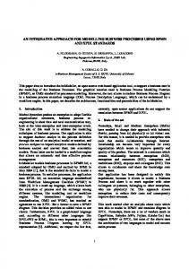
Figure 1: The proposed modelling paradigm. served their purpose, we need to consider another taxonomy that ts more closely with related modelling eorts in the AI and SE communities. The modelling of dynamic systems has become a widespread phenomenon and is no longer speci c to the simulation discipline; we need to embrace these competing areas to derive a common taxonomy or \world view" with regard to system modelling. This alternative taxonomy is based on a set of modelling approaches depicted in gure 1. In g. 1, the rst type of model is the concept model which corresponds to an object model within SE or a system entity structure [91]. The concept model is non-executable, and serves as a knowledge base for the system. From the concept model, one can derive either one of two basic modelling forms: declarative and functional. Declarative models emphasize state transitions, while functional models emphasize operational or event oriented modelling. Declarative and functional model forms are prevalent in all three disciplines. For instance, programming languages are often categorized into either declarative [1, 49] or functional [48, 6] types. The declarative programming languages (such as Prolog) emphasize changes in state where \states" are best coded as particular data structures | a simple variable being the most commonly used form for a state. Functional programming languages concentrate on functional composition while de-emphasizing side eects2. One may combine these forms to synthesize heterogeneous models where model graph nodes may be of dierent types. Finally, the multimodel [33, 57, 37] is the most comprehensive type of model that supports multiple models tied together with homomorphic mappings from one model to another [28]. The multimodel approach is a generalization of combined simulation modelling [18, 71] where models may be of many dierent types | not just a mixture of discrete event and continuous components. The proposed taxonomy is an extension to the object oriented modelling paradigm. While we adhere to the object model as a good basis for conceptual, non-executable models, we depart from the norm 2

The \side eects" for software encoding dynamical system behavior are actually the states of the system.

CIS TR92-006 TBP:


4

when introducing how additional modelling techniques such as production systems, trackbased animation and System Dynamics t within the overall framework. In the usual object oriented modelling approach within SE [79, 16], speci c modelling methods such as FSA modelling and DFDs are promoted. We treat these two types of models as instances of a class rather than a class by itself. Our approach is to stress the utility of having functional and declarative classes of models. In our declarative modelling class, for instance, we list several types of models including FSAs, production rules, and logic based models. We are interested in overviewing the commonalities in the modelling process as well as asking fundamentally interesting historical questions such as \What are the causes or catalysts aiding in the relatively recent convergence in AI, SE and simulation modelling?" and \How, precisely, will modellers and decision makers bene t in this convergence?" The integrated style is being used by several simulation researchers [92, 60, 78, 66, 33, 3]; however, it has not yet penetrated the general simulation textbook literature as a more powerful paradigm for modelling dynamical systems. Although the introduction of new dichotomies, taxonomies and reorganizations is a philosophical issue, we have had rst hand experience in teaching the proposed simulation modelling methodology to college seniors and rst year graduate students at the University of Florida with much success. Students who take, for instance, courses in AI and SE can take a class in simulation that builds upon |rather than replaces| recently learned model forms. Two key aspects of the view shown in g. 1 are the declarative versus the functional perspectives. These two modelling views form a dichotomy in that most modelling methods in simulation are oriented toward one view rather than the other. System Dynamics models [74] and block models, for instance have functional orientations. The term \dichotomy" is used somewhat loosely, though, since there exist several kinds of modelling methods such as Petri nets [70] that have equal shares of declarative (i.e., place) and functional (i.e., transition) sub-representations. We rst overview why we chose these two categories in our attempt to synthesize system modelling techniques in AI, SE and simulation. Within the context of a two jug problem in AI, we then discuss how the jug system can be viewed from these two perspectives. Finally, the multimodel approach is illustrated to demonstrate how models of dierent types may be coupled together to form a multimodel or \model database." We close with some conclusions and research currently underway to extend these ideas.

2 Synthesis of Modelling Techniques 2.1 AI & Simulation Models

Within AI, one is concerned with how to model human thought and decision making. Often, the decision making is heuristically based, and there is incomplete knowledge about the domain [56]. This \incompleteness" should be programmed into the dynamical model where it is present. For the past decade, the interface area between AI and simulation has grown, and several papers and texts have appeared [63, 64, 84, 36, 43]. Simulation models have characteristically been composed of simple entities and objects; however, the introduction of autonomous agents within the queue into a model has suggested that simulationists use AI

CIS TR92-006 TBP:


5

models in places where autonomy is present. While a simple queuing network avoids the use of knowledge based simulation models, a more detailed model would include beliefs, plans and intentions of the autonomous agents |in the queue| at some level of detail. Trajectories of projectiles and three phase motors are comparatively simple to model because these objects operate in accordance with natural laws that are controlled through engineering; the laws and control methods for non-autonomous objects are fairly simple with regard to model complexity. Models of intelligent agents are much more complicated due to the sophisticated reasoning abilities of humans and of robots that are endowed with human-like reasoning. Autonomy has, therefore, spawned the creation of knowledge based models that contain a variety of natural, arti cial and intelligent objects interacting and reasoning in a complex environment. The elds of qualitative reasoning and qualitative physics [83, 13] are evidence of the AI interest in system modelling from the perspective of mathematical reasoning. In addition to autonomy playing a critical role, incomplete knowledge is ever present within models and AI researchers have suggested new ways of representing this type of knowledge. While simulationists have used probability theory for representing abstracted quantities, one can also use heuristic rules and constraint based modelling techniques. These types of techniques have been used for declarative and functional modelling [85]; however, they are most useful within conceptual models that serve to enhance our ability to diagnose symptoms, plan future actions and provide common-sense explanations of device behavior [83, 22].

2.2 SE & Simulation Models

Software engineers are pioneering new and novel methods for building system models; tools such as Foresight [5] provide the modeller with the capability of modelling dynamic systems using nite state automata and block modelling all under the umbrella of object organization. Software engineers have developed a keen interest in simulation; there is an apparent convergence between these two areas [76, 68, 7, 8, 61, 45, 46]. Some of our previous research [31, 30, 32, 37] has suggested the study of model engineering as a direct analog to software engineering. Within the simulation community, Zeigler presents a theory for modelling autonomous agents [92] while implementing a model engineering methodology. The historical reason for the convergence of the SE and simulation elds lies in the area of distributed and real-time design [72] and computing. Technology has seen the computer decrease in size and cost while increasing in power. This combination of circumstances naturally leads to the use of computers in almost every electro-mechanical device. When software engineers had to concern themselves with modelling only mainframe or workstation software, the modelling process dealt with functional decompositional methods: creating hierarchical routines and stubs while gradually expanding the size and complexity of the program. Now, however, with the ever expanding migration of the microprocessor, the structural components of software models are beginning to act and appear like the physical objects in which the processors live. Modelling distributed software, with its emphasis on communication protocols, is similar to modelling the physical objects for which the software is written. Thus, the convergence of SE and simulation models stems largely from distributed computing. There are key dierences, though, between the end results one obtains. Software engineers want an executable program, while simulationists want to model the performance and lumped behavior of the system. While these two avenues appear to diverge, there is

CIS TR92-006 TBP:


6

actually a con uence. The con uence is best seen at a higher level in the decision making process that oversees the use of software engineers and simulationists. That is, the decision maker who wants to create ecient and correct distributed software for his inter-bank transaction project, for instance, is also highly concerned with the eciency of the entire distributed architecture. Whereas, a decade ago, a project might have involved simulation before or during actual construction of hardware, communications pathways and distributed software, now a project can be created while cleanly integrating the tasks of performance analysis with software development. The ultimate simulation is the actual creation of the software which is then executed; lumped statistical behaviors can easily be obtained when one has the lowest level performance traces. The ultimate software development tool is one that permits modelling the software at a variety of abstraction levels | the lowest level providing detailed behavior of the sort normally associated with program input and output traces. Given this view, simulation is the process of creating abstract versions of programs; the nal most detailed simulation is simply the executable program.

3 Terminology

3.1 Using Systems Theory as a Starting Point

For the fundamental building primitives comprising models that represent time-dependent system behavior, we have found systems theory [69, 87, 52, 51] to provide the most mathematically consistent foundation. Systems theory has developed since the early 1960s into a eld that made precise the core components of \systems" regardless of the speci c discipline (i.e., computer science, biology, chemistry, physics, operations research) [12, 4]. The rst formal theories for discrete event simulation [88, 89, 91] were founded upon systems theory, and much recent work has continued this trend. Even though our proposed paradigm is consistent with object oriented modelling, we were surprised at the lack of system theoretic formalism present in AI and SE general; the formal emphasis within SE seems to be within formal veri cation and correctness of programs. AI has many formalisms of which mathematical logic is the most prominent. On the other hand, simulation literature is relatively weak in its use of logic and in its emphasis on correct programs implementing models; however, recently there has been renewed interest within the use of logic to both verify and simulate models [62].

3.2 The Generic Model Structure

A deterministic system < T; U; Y; Q; ; ; > within classical systems theory [69] is de ned as follows: T - is the time set. For continuous systems [19], T = R (reals), and for discrete time systems, T = Z (integers). U - is the input set containing the possible values of the input to the system. Y - is the output set.

CIS TR92-006 TBP:


7

Q - is the state set. - is the set of admissible (or acceptable) input functions. This contains a set of input

functions that could arise during system operation. Often, due to physical limitations,

is a subset of the set of all possible input functions (T ! U ). - is the transition function. It is de ned as: : Q T T ! Q. is the output function, : T Q ! Y . A system is time invariant if its behavior is not a function of a particular interval of time. This simpli es to be of the following form: : Q T ! Q. Here, (s; t; !) yields the state that results from starting the system in s and applying the input ! for a duration of t time units. This formalism, although concise, is quite general. For structural reasons we employ techniques such as level coupling, inter-level coupling and hierarchy to make the overall system more manageable; however, we rst identify some key pieces within the above de nition. Q is also known as the state space of the system. An element s 2 Q is termed the state of the system, where the state represents a value that the state components can assume. The state of an ice hockey puck would be (x; y) whereas the state of a two-queue system would be (q1; q2) where qi represents the number of entities in queue i. Normally the state has a structure of an n-tuple: fs1; s2; : : : ; sng however, it is best generalized as a data structure | a tuple being one type of data structure. Superstates provide exibility in describing some model forms [35]. A superstate is a subset of a state, therefore, \goal" is the subset of the hockey puck state representing the geometrical region where the goal net is located3. A pair consisting of a time and a state (t; s) where s 2 Q is called an event. Events are points in event space just as states are points in state space. Event space is de ned as Q T . Events normally represent values of state that correspond to de nite cognitive or lexical mappings [10, 11]. For instance, in a queueing model we identify an event as an \arrival" but we may not have words to represent the values of other states whose values do not correspond to a cognitive or lexical association. State and Event are critical aspects of any system and by focussing on one or the other, we form two dierent sorts of models: declarative models that focus on the concept of state, and functional models that focus on the concept of event. States represent a \snapshot" of a system, while events, even though they occur at points in time, are naturally associated with functions (i.e, routines, procedures). A change in state is associated with an event, and vice versa; so, there is a duality between states and events. Declarative and functional orientations are discussed widely in both AI and SE, and we propose that they share a common bond with simulation modelling as well. Given basic elements such as states and events, we can structure models in various ways to aid us in better analyzing systems. By coupling functions or states, and by making networks and hierarchies we can simplify the overall model organization. We will call one model an \abstraction level" or a \perspective." Abstraction levels are discussed by many researchers in SE [58], AI [82] and simulation [28, 29]. A model can contain homogeneous or heterogeneous node types; simple modelling constructs are homogeneous (such as FSAs), and more complex constructs are heterogeneous (such as System Dynamics graphs, Petri nets or 3

The concept of superstate in SE is discussed by Davis [21]

CIS TR92-006 TBP:


8

bond graphs). If the hierarchical organization is not purely representational (i.e., all levels can be collapsed into a single model) then we can have multimodels where many models are attached to one another via behavior-preserving homomorphic links.

4 Concept Models Models whose components have not been clearly identi ed in terms of system theoretic categories such as state, event and function are called \concept models" [81]. Conceptual models are a logical rst step to modelling; research in these models has many connections in AI, SE, systems science and simulation. At rst, it would appear that non-executable models should play no part in simulation. Simulationists have historically not spent a considerable amount of time on \model engineering" (with exceptions noted in the previous section); even though the need for iterating through the modelling process is well understood and appreciated, there is little textbook methodology present to aid simulationists in this key area. Model engineering does not lend itself to a nice neat formalism, and therefore the engineering aspect of simulation modelling is often part art and part science [80]. Despite this diculty in formalization, model engineering is a critical task and should be a central activity within the simulation eld; we want to better understand the very nature of modelling including how and why we choose the models that we do during the course of systems analysis. The area of Systems Dynamics [42, 41, 74, 75] focuses, not only on the formalism for a dynamic model but also, on several key steps during the model building process: 1) causal model without signed information, 2) causal model with signed arcs and loops, 3) ow graph, and nally 4) equations (or program). These steps provide clues as to how we might engineer more generic models. This is not to suggest that we should abandon all of our modelling methods in favor of the Systems Dynamics approach. Instead, we note that one success of the approach is its clearly emphasized model engineering steps. The rst type of model that we want to create is a concept model that emphasizes a objects and their relations to one another. From such a model, we can gradually progress to more system theoretic constructs. The concept model in AI is termed a semantic network [86, 27, 17], while equivalent model in SE is the object model with attribute de nition [79, 15, 16, 14]. Most work in simulation, concerning concept models, has been performed along the lines of model speci cations [59, 68] and the system entity structure [89, 92]. Since simulation has its formal roots in systems theory and science, we nd work relating to conceptual modelling in these areas as well [20, 52, 38]. The semantic network, even though it can serve as a rough cut of a simulation model, was often built as an end in itself, or to facilitate qualitative reasoning via link traversal. Semantic networks are traversed to answer simple questions about a system. Simulationists need such models |to augment their mathematical system models| since there is often a need to ask more than simply \predict when object XYZ reaches point B" or \give the mean idle time for the cashier." It would also be useful for simulationists to be able to ask more abstract questions about a system, and furthermore, to obtain abstract answers that serve in forming a causal explanation of system behavior [77]. The typical AI semantic network would be very weak at producing precise quantitative answers; however, similar claims can be made against an equational simulation model | it produces precise answers but cannot produce simple explanations of behavior in \close-to"

CIS TR92-006 TBP:


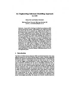
Jug A 3 gallons

9

Jug B 4 gallons

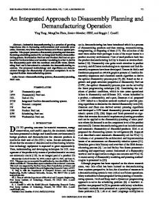
Figure 2: Two jug system. natural language expression. Therefore, concept models not only provide a \speci cation" for a simulation model, they are simulation models at high levels of abstraction. The object modelling approach in SE has produced the equivalent of the AI semantic network, but for a dierent purpose: to permit a software engineer to prototype a large software system. Our approach is similar to object oriented design principles espoused in SE: begin with an object representation and then produce declarative and functional model types. Let's consider the water jug problem in AI [53, 73]. In the water jug problem, there are two water jugs (one with a three gallon capacity, and the other with four gallons). Jug A is the three gallon jug and jug B is the four gallon jug (see gure 2). There are water spigots and no markings on either jug. There are three basic operations that can be performed in this system: emptying a jug, lling a jug, or transferring water from one jug to the other. A concept model can be created by concentrating on key objects, concepts and actions within the system. Rumbaugh et al. [79] present a useful checklist for deriving the object model: 1. Identify objects and classes. 2. Prepare a data dictionary. 3. Identify associations and aggregations among objects. 4. Identify attributes and objects and links. 5. Organize and simplify object classes using inheritance. There are no hard rules for developing an object model; however, this checklist serves as a starting point by suggesting guidelines. The complete process would involve iterative re nement of the rules. Let's consider each guideline with respect to the two jug system. An object graph will be composed of vertices and arcs, so we start by de ning the nodes. Objects will be considered either classes, which de ne broad categories, or instances, which de ne examples within classes. Nouns are often a good place to start when identifying classes. For instance, the noun \tap" is a good class since there are many dierent types of taps including the two used in the system. If we use the statement of the system description, we arrive at the following classes: tap and container. We consider tapA and tapB to be examples of

CIS TR92-006 TBP:

ACM Transactions on Modeling & Computer Simulation, V2, N4 10 controls (fill)

Agent Name

controls (empty,xfer)

Tap

Container

Rate

Capacity

Jug

Barrel

Level

Dimensions xfer

empty Ground Elevation

Figure 3: Class model: two jug system. a tap, and jug and barrel to be sub-classes of container. JugA and JugB compose every known jug in this closed \world." We can then create a data dictionary where encyclopedic information about the classes and instances are stored. Our associations often take the form of verbs or operations associated with the system; therefore, ll, empty and transfer are natural selections for associations. The choice of attributes depends on the kinds of questions that we will be asking of the system. If we will |in the section on declarative modelling| de ne the operations in terms of integral amounts of water, then level of water and rate of water ow will be key attributes. After some additional iteration we arrive at the concept and instance models depicted in gures 3 and 4.

5 Declarative Models In declarative modelling, we build models that focus on state representations and state-tostate transitions: given a state and a transition, the model will provide the next state. This

CIS TR92-006 TBP:

control (fill)

ACM Transactions on Modeling & Computer Simulation, V2, N4 11

Tap B

Tap A

rate

rate fill B

fill A

control (xfer,empty)

control (fill)

Jug A level

Xfer

Jug B level

Xfer

empty A

empty B

Ground

Figure 4: Instance model: two jug system.

control (xfer,empty)

CIS TR92-006 TBP:


simple metaphor provides for a whole class of models. The FSA and Markov models in simulation are the most basic declarative model types.4 In SE, the state transition model is termed the \dynamic" or \state" model. Harel [44] extends the basic state model to form state charts containing embedded hierarchies of FSA levels. The use of the word \dynamic" is somewhat unusual from a simulationist's perspective since data ow diagrams are also a valid form of dynamic model representing input, transfer functions and outputs coupled within a block network diagram. On the other hand, in SE, the reference to \dynamic" re ects that state change is at the heart of dynamics. This is in agreement with systems theory and all three disciplines although memoryless functions can also represent dynamical systems. Moreover, if FSAs are embedded within another formalism (such as a data ow diagram) then that formalism is also considered dynamic. In AI, the declarative approach to system modelling is quite advanced since there are several AI declarative representations that can be useful in modelling. From AI, we can enrich the state-oriented declarative modelling approach to include logic, rules, and production systems. The declarative approach need not be limited to simple state to state transitions. For instance, in AI we often nd pattern matching or constraint approaches in the uni cation process present within logic programming; pattern matching over a state space Q provides a convenient method of de ning superstates (i.e., subsets of state space). For instance, if Q = X1 X2 for a two dimensional hockey rink then the goal net location could be speci ed by the constraint f(X; Y )jY 10g. Logic programming and, especially, constraint based programming [55, 47] typify the declarative approach to modelling using state space partitions to create superstates. The production system, constraint and logic approaches utilize uni cation and pattern matching to aord declarative methods the capability of representing complex behaviors with a modicum of mathematical notation. Methods of production systems [23] and formal logic [26] (either standard or temporal) may be used as a basis for simulation modelling. We need to de ne the concept of state, input and time with respect to these models: State is de ned as the current set of facts or truths in a formal system. For predicate logic this equivalences to a set of predicates. For expert systems, the rule or \knowledge" base is the state of the system. For production systems, inputs are known as \operators" which are executed by the controlling agent. A sequence of parameterized calls to the operators serve as the input stream that controls the system. We will associate time durations with input events by saying that whenever an input event occurs (which causes a change in state), the ensuing state will last for some speci ed period of time. Time can be assigned to each production or inference so that the process of forward chaining produces a temporal ow. We could make state variables vary continuously or discretely. The state of the water jug model will be identi ed by a set of predicates. Note that predicates and arguments are both in lower case. The state is de ned as (X; Y ) where X is the amount of water (in gallons) in the 3 gallon jug, and Y is the amount of water in the 4 4

In systems theory, the the FSA is sometimes termed a \local transition function."

CIS TR92-006 TBP:


gallon jug. We de ne states to vary using discrete jumps so that lling an initially empty jug A, for instance, would cause a jump from state (0; 0) to (3; 0). We will assume an initial state of (0; 0) (i.e. both jugs are empty). Time will be measured in minutes, therefore rates are measured in terms of gallons per minute. Filling is somewhat slow and proceeds at a rate of 2 gallons per minute. All other operations take 10 gallons per minute. There are 4 operators de ned as follows: The operator and description. Conditions for the operator to be applied (i.e., re). The time duration T of the operator if it is applied. The duration is associated with the current state. 1. OPERATOR 1: empty(J ). (a) Empty jug J 2 fA; B g. (b) For J = A, (X; Y jX > 0) ! (0; Y ) and T = X=10. (c) For J = B , (X; Y jY > 0) ! (X; 0) and T = Y=10. 2. OPERATOR 2: fill(J ). (a) Fill jug J 2 fA; B g. (b) For J = A, (X; Y jX < 3) ! (3; Y ) and T = (3 ? X )=2. (c) For J = B , (X; Y jY < 4) ! (X; 4) and T = (4 ? Y )=2. 3. OPERATOR 3: xfer all(J 1; J 2). (a) Transfer all water from jug J 1 to jug J 2. (b) For J 1 = A, (X; Y jX + Y 4 ^ X > 0 ^ Y < 4) ! (0; X + Y ), and T = X=10. (c) For J 1 = B , (X; Y jX + Y 3 ^ Y > 0 ^ X < 3) ! (X + Y; 0), and T = Y=10. 4. OPERATOR 4: xfer full(J 1; J 2). (a) Transfer enough water from jug J 1 to ll J 2. (b) For J 1 = A, (X; Y jX + Y 4 ^ X > 0 ^ Y < 4) ! (X ? (4 ? Y ); 4), and T = (4 ? Y )=10. (c) For J 1 = B , (X; Y jX + Y 3 ^ Y > 0 ^ X < 3) ! (3; Y ? (3 ? X )), and T = (4 ? Y )=10. The application of various operators will change the current state to new state. For instance, given the initial system state as being (0; 0) we see that we can apply only operator fill. Speci cally, we can do either fill(A) or fill(B ). Both operations take a certain amount of time T . The T is associated with the current state. Let's look at the time taken to ll jug A. We note that the production rule associated with this operation is: \For J = A, (X; Y jX < 3) ! (3; Y ) and T = (3 ? X )=2." To go from state (0; 0) to (3; 0), for instance,

CIS TR92-006 TBP:


will take a total time of T = (3 ? 0)=2 or T = 1:5. This is interpreted as: \if the system is in the state (0; 0) and the operator ll is input to the system then the system will enter state (3; 0) in 1:5 minutes." In other words, the system remains in state (0; 0) for 1:5 minutes before immediately transitioning to state (3; 0). If we consider each operator as representing an external, controlling input from outside the jug system, then we can create a an FSA that represents the production system. Figure 8 displays this FSA where the following acronyms are de ned: 1. Ex: Empty jug x. 2. Fx: Fill jug x. 3. TAxy: Transfer all water from jug x to jug y. No over owing of water is permitted. 4. TFxy: Transfer all water from jug x to jug y. until jug y is full. Even though the state space contains 20 states there are only 14 possible states in the FSA. The two jug system dynamics are quite complex; this attests, primarily, to the power of production rules (with pattern matching) over simple FSAs (without pattern matching). We can simplify the system by partitioning state or event space. There is no automatic method for state space partitioning; however, we can use a heuristic to help us: form new states using participles created from the object model. That is, the present participle form of \ ll" is \ lling." A similar approach creates the state \emptying." We can combine both the emptying state and lling state to form a stated called In-between or Emptying-or- lling. Figures 5 through 7 suggest a partitioning of state space that provides a lumped, more qualitative model. Since these segments overlap, and do not form a minimal partition, we must combine substates |re ecting levels in jugs A and B| to form 9 new states. The greatest \lumping" eect is contained in the state (Jug A lling, Jug B lling) where the term \ lling" means neither empty nor full. It is important not to underestimate the lumping eect when considering other possible, but similar, systems. For instance, if the jugs could contain arbitrarily large amounts then the state space for g. 8 would also be large, but the state space for the lumped model would remain the same (9 states). It is possible to further reduce the number of states by mapping and partitioning state or event space in accordance with natural language terminology; state space could easily be broken into \wet" and \dry" where dry corresponds to both jugs being empty, and wet covering the remainder of state space. Models at varying levels of abstraction [29] are created in response to the questions asked of them [37].

6 Functional Models We will use a liberal interpretation of the word \functional" to include modelling approaches that stress procedural or \process-oriented" models [34]. A purely functional model is termed \memoryless" since there is no state information; so we de ne a functional model as one that focuses on \function" rather than state to state transition. Functional models, therefore, will often contain FSAs embedded within the de nition of a functional block; the model is considered \functional" if this view dominates any subsidiary declarative representations. A

CIS TR92-006 TBP:


Jug B

Jug B

4

4

3

3

2

2

1

1

0 0

1

2

3

Jug A

0 0

1

(a) Jug A full.

2

3

Jug A

(b) Jug B full.

Figure 5: Full phase.

Jug B

Jug B

4

4

3

3

2

2

1

1

0 0

1

2

3

Jug A

0 0

(a) Jug A empty.

1

2

3

(b) Jug B empty.

Figure 6: Empty phase.

Jug A

CIS TR92-006 TBP:


Jug B

Jug B

4

4

3

3

2

2

1

1

0 0

1

2

3

(a) Jug A In-between.

Jug A

0 0

1

2

3

Jug A

(b) Jug B In-between.

Figure 7: In-between phase. function will be represented as a block with inputs and outputs. Inputs and outputs can represent data ows or control ows, and they are de ned as such within SE [5]. From our perspective, these ows are all data ows regardless of whether a function treats its input data from a control perspective. The functional SE box structuring techniques of Mills [58] bear remarkable resemblance to those of systems and simulation theory [69, 88]. This further demonstrates a convergence in model theory between SE and simulation. If we consider each tap and each jug to be a function then we can create a functional block model illustrated in gure 9. This dynamical model could be simulated as it is represented; that is, messages would be input to blocks that would delay the corresponding outputs to represent the passage of time. Use of a delay, therefore, represents a simple way to create an abstract model. If we want to increase model detail, the delay can be further decomposed into an FSA. For the tap dynamics, we use a delay; however, for the jug dynamics, we choose an FSA. The dynamics for jug A are shown in gure 10. The entire functional model shown in g. 9 has four functional blocks with two of the blocks (jugs A and B) having an internal FSA to further re ne state to state behavior. It is worthwhile to contrast this model with the declarative model in g. 8. In the declarative model, each state represents the state of the entire system whereas, for the functional model, states are \local" to the speci c function. In the object oriented sense, these states are hidden or encapsulated within the block. The aspect of locality is what has made the functional approach more acceptable to the systems community | a system is broken into functional blocks, each of which represents a physical subcomponent of the system, and each subcomponent has its own dynamics. The declarative approach of a rule-based production system |while it accurately represents the jug system


CIS TR92-006 TBP:

E1 3,0

TA21

F2

0,0

E2

F1

0,4

TF21

F1

TA12

F2 0,3

E1

T12 E2

E1 F1

3,4 F2

E2

3,3 TF21

E2

E1

3,1

F2

TF12

E1

E1

E1

F2

2,4 F2

2,0

0,1

E2

E2

TA12 TA21

F2

1,0

TA12 E2

TA21 0,2

F1 E1

TF12

1,4

3,2 TF21

Figure 8: FSA for the jug system.

F2

E2

CIS TR92-006 TBP:


Control (Fill)

Tap A

Tap B Fill B

Fill A

Control (Xfer,Empty)

Control (Fill)

Xfer

Jug B

Jug A

Control (Xfer,Empty)

Xfer Empty A

Empty B

Figure 9: Functional model of two jug system. Fill(A)

Jug A X=0

Xfer(A,B) Empty(A)

(0,Y) Empty

(X,Y) Empty(A) 0