from reaching the wall and cooling. The closed geometry ..... the-fly parameter culling, we can specifically select a small subset of particles to .... coordinates and the grand tour,â Computing Science and Statistics 28, pp. 361â368, 1997.
1
An Integrated Exploration Approach to Visualizing Multivariate Particle Data Chad Jones, Kwan-Liu Ma, Stephane Ethier, and Wei-Li Lee
Abstract—Particle simulations are powerful tools for understanding the complex phenomena associated with many areas of physics research, including confined plasma and high energy particle beams. Analyzing the data, however, presents a challenge due to the large quantity of particles, variables, and time steps. In this paper we describe a data exploration system that visualizes time-varying, multivariate point-based data from gyrokinetic particle simulations. By utilizing two modes of interaction (physical space and variable space) the system allows scientists to explore collections of densely packed particles and discover interesting aspects of the data. We employ a parallel-coordinate interface for interactively selecting particles in multivariate space. In this manner, particles with deeper connections can be separated from the rest of the data. From the results of this system, we are able to identify features of interest, such as the location and motion of particles that become trapped in turbulent plasma flow. Index Terms—Particle visualization, multivariate visualization, information visualization, user interfaces, parallel coordinates.
I. I NTRODUCTION When studying complex phenomena, scientists often employ numerical simulations or experiments to isolate and understand possible contributing factors. Depending on the needs of the simulation, various types of data (such as scalar, particle, or vector fields) may be collected. Our application focuses on exploring particle data, which is often used to capture time-dependent changes in simulations from many fields of study, including material science and physics. The features of our approach are demonstrated using data from plasma physics simulations. Plasma physics is rich in complex, collective phenomena and encompasses major areas of research including plasma astrophysics and fusion energy science. As part of their mission to develop practical fusion energy, the scientists at the Princeton Plasma Physics Laboratory (PPPL) have made extensive use of particle-in-cell simulations to advance the understanding of energy and particle transport in fusion devices called tokamaks [1], [2]. The loss of energy due to transport out of the hot plasma core is believed to be due to microturbulence that develops under driving pressure gradients, and simulations can lead to the discovery of new ways to control and prevent these losses. This complex phenomenon is best simulated by the particle-in-cell method. Positions and velocities of sample particles are followed in time as they interact with the self-consistent field that they produce and C. Jones and K.-L. Ma are with the University of California at Davis and the SciDAC Institute for Ultrascale Visualization., E-mail: {cejjones, ma}@ucdavis.edu. S. Ethier and W.-L. Lee are with Princeton Plasma Physics Laboratory, E-mail: {ethier, wwlee}@pppl.gov.
with the externally imposed confinement magnetic field. With simulations using over a billion particles, the amount of data produced can truly be overwhelming. Traditional analyses for these simulations have been limited to the evaluation of macroscopic quantities such as the heat and particle fluxes in different regions of the plasma, the field energy, the flows, and other derived quantities calculated using the moments of the particle distribution functions. The resulting visualizations have been mainly X-Y plots, with a few contour plots being evolved in time. Modern, multidimensional visualizations of fundamental particle quantities, such as the ones being introduced in this paper, elevate the analysis to a whole new level for the fusion scientists. Although unfamiliar with these new ways of exploring data, scientists can more effectively confirm or discover properties of their data that could not be seen before. To solve the challenges that data exploration poses, an application must provide an understanding of the particles on both global and refined scales. Traditional scientific visualization techniques for rendering particles in physical space provide an understanding of key spatial relationships among variables, but a global understanding of multivariate connections is difficult to convey as no intuitive representation of multidimensional data exists with physical 3D rendering. By integrating multiple representations of the data, including techniques developed for information visualization, we can alleviate the limitation on expression and control. From a top level view of the data, scientists can interact with various parts of the visualization to select groups of particles with specific multi-dimensional connections. The multivariate aspect of selection is handled via parallel coordinates; selected variables are highlighted, combined with logical operators, or modified across time. Based on the mode of selectionlock, the group of particles examined across time may differ. Scientists, in turn, obtain the ability to examine multiple timedependent features. Physical space visualization remains an important way to discover properties of particles based on location and motion. All of these views culminate in a final data exploration interface. A modification to any one particular view updates the appearance of all views, which focuses the visualization on the subset of interest. Linking the views is essential for revealing properties of the particles that may be illusive through previous means of particle visualization. Based on initial results, our system has provided scientists at PPPL the ability to explore connections between multiple particle variables, both fundamental and derived. Complicated groupings that would be otherwise difficult to isolate become easy to discover using a multiple-view approach of visualiza-
2
tion and interaction. With this system, visualization enhances the study of new particle simulations, and scientists concerned with particular phenomena can quickly uncover and display particles of interest. II. BACKGROUND AND R ELATED W ORK Our system builds from several areas of visualization research, including particle rendering, multivariate visualization, and parallel coordinates. This section discusses relevant background and related work. A. Particle Visualization Several research areas take advantage of particle representations for numerical simulations, and important advancements have been made to better visualize such point-based data. Ma et al. [3] used terascale neutron particle accelerator data to introduce techniques for visualizing both particle beam data and magnetic field lines. In order to improve interactivity of the particle visualization, they created a hybrid approach that combined texture-based volume rendering in areas of low interest and point-based rendering in areas of high interest. Particles are normally rendered by small glyphs, such as spheres. Kruger et al. [4] implemented a particle engine that uses the GPU for sorting and rendering particles as shaded points and oriented texture splats, which are then applied to 3D flow fields on uniform grids. Improvements have also been made to the perception of particles by more effective shading and illumination [5]. Our analysis of particles requires the ability to easily filter with color, opacity, or selection culling. We thereby utilize techniques that simplify the identification of individual particles, even out of dense clusters. B. Parallel Coordinates For the purpose of visualizing multiple variables, our system takes advantage of parallel coordinates. Since being introduced by Inselberg [6], they have been widely used for visualizing relationships among multiple variables. The technique creates a vertical axis for each data dimension. For each data element, a polyline is drawn to intersect every axis based on the element’s value for that variable. Many of the advantages, such as conveying patterns, outliers, and features, are lost when the parallel coordinates are applied to large scientific data. One way to reveal clusters in a cluttered parallel coordinates was proposed by Wegman and Luo [7]. They used translucent lines to fade away sparse areas while highlighting dense areas. Novotny and Hauser [8] addressed the issue of outlier preservation for parallel coordinates by handling outliers and trends separately. Their technique has successfully helped visualize up to 3 million elements. We use parallel coordinates to handle the selection of particles based on multivariate conditions via range selection and combination operators. Different locking mechanisms provide the ability to see changes over time or modify the existing selection at another time step.
C. Multivariate Interfaces One common approach to addressing the challenge of multivariate data exploration is the integration of several views into a single interface. In this area, two recent works have utilized parallel coordinates to provide a multidimensional means for exploring complex data. The work presented by Akiba et al. [9] provided an interface for exploring multivariate, time-varying volume data. Their interface used parallel coordinates and time histograms to specify multivariate and time-varying transfer functions. Rubel et al. [10] developed an application called PointCloudXplore, which links physical views with parallel coordinates to study 3D gene expression data. Unlike the previous work, our interface focuses on the exploration of particle data based on multi-dimensional inquiry. Similar to recent work, however, our approach takes advantage of parallel coordinates to handle multiple variables and provides ways of combining, locking, and brushing multiple ranges to actively drill down into data. The drawbacks of individual visualizations are overcome by linking multiple views of the data together. III. G YROKINETIC PARTICLE S IMULATIONS The main goal of gyrokinetic particle simulations is to study anomalous energy transport associated with plasma microturbulence. By employing 3D gyrokinetic particle-incell simulation code, studies of plasma microturbulence have dramatically improved the knowledge of instabilities and their effect on plasma confinement. To sustain the required high temperature for fusion reactions, the plasma particles must be confined using a strong magnetic field, which prevents them from reaching the wall and cooling. The closed geometry containing the necessary properties for plasma confinement is the torus, which is the geometry of all current fusion devices. Gradients of temperature, density, and the magnetic field thereby generate complex particle motions and drive turbulence in the plasma. PPPL’s Gyrokinetic Toroidal Code (GTC) is a full-torus, global gyrokinetic code developed to study these phenomena and has already lead to many new insights [2]. One type of data set that is outputted by the simulation is a Maxwell potential data in a scalar volume. Crawford et al. [11] developed a hardware accelerated volume visualization approach to render the scalar potential data of gyrokinetic simulations. Their key insight was to introduce a transform from the irregular torus shape into an unwrapped square-toroid texture. The ability to explore the time-varying, multivariate particle data, however, is an area of great interest that can benefit from new visualization techniques and user interfaces. Besides providing a global view of the data, isolating subsets of particles based on multivariate properties is a highly desirable feature when only a small number of particles represent the aspect of interest. For example, the concept of particle trapping in magnetic confinement devices is crucial for understanding energy and particle transport. As particles move along the magnetic field lines in a fast spiral motion, they go through regions of increasing magnetic field strength and energy is transferred from parallel motion to perpendicular
3
motion. When the particle energy is below a certain threshold, the parallel velocity approaches zero in the strong field region and the particle changes direction, exhibiting a back-and-forth motion characteristic of a trapped particle. Above the energy threshold, the so-called passing particles continually circulate around the torus without changing direction. The magnetically trapped particles have a much greater impact on transport than the passing particles. Studying this property in a visualization system would be difficult without a way to separate those particles from the larger set. IV. PARTICLE E XPLORATION S YSTEM Unlike analytical and numerical calculations, which are the traditional methods for studying simulation data, a visualization system can provide a visual means to explore and understand the data. The tool must adapt to changing scientific inquiries by providing a way to isolate subsets of the data, reduce the dimensionality of the visualization, and present it in a more familiar fashion. Our system addresses the multivariate problem by providing both variable and physical views of the data. The variable visualization is not only used to show the relationships and trends among the many variables, it also provides an intuitive interface for selecting data items. The physical visualization, however, shows a spatial representation of the data via advanced rendering techniques. Sections IV-A and IV-B describe the representations of the particle data, and section IV-C explains linking and interaction of the views. A. Particle Visualization The physical view is represented using either spherical glyphs for a single time step or illuminated pathlines for a range of time steps. In both cases, a single scalar variable, chosen interactively by the user from a list, is mapped to color and opacity for that primitive using a one-dimensional transfer function. 1) Particle Rendering: We have provided the ability to render points with a spherical shape, which improves rendering quality and depth cues over normal point rendering. To sustain interactive rates, we utilize view-aligned billboards using hardware-supported point sprites, which has previously been used for flow particles and material point method data [4], [5]. Particles are still represented by a single vertex position, but the glyph shape can be controlled via a two dimensional texture, which is typically a circle. Hardware shaders provide this circle with a spherical appearance by applying sphere lighting calculations to the surface. As Figure 1 shows, the color and opacity for each particle are controlled by a 1D transfer function. A standard freeform transfer function widget allows the user to view a histogram of the data, draw an opacity function, and define multiple color nodes over the data values. Since we utilize transparency, the particles must be sorted before rendering [4]. In terms of memory usage, point sprites do not require any additional storage because the particle positions can be used directly during the rendering stage. The size of the glyphs can be interactively increased or decreased depending on user preference or to reduce overlapping problems. The user may
also define the size of a particle to vary with some condition, such as statistical weight. 2) Illuminated Pathlines: Shaded point sprites provide a detailed view of static particles at a single time step. Animating the particles over time can provide a basic understanding of motion, but tracking individual particles trajectories beyond a few time steps is difficult. Rendering particle trajectories as pathlines is another potential solution. To be effective, this rendering style must be both visually informative and interactive. As a result, we utilized the current advancements in illuminated line rendering [12], which is an acceptable tradeoff between rendering quality and performance. To show changes in value over time, pathlines are colored by the same transfer function that is used for particles. Less important values can be made more transparent to hide unwanted visual information. The illuminated pathlines are sorted amongst themselves to provide correct blending [12]. Significant speedups are achieved by storing the vertex and color information in vertex buffer objects. The user can interactively adjust the forward and backward length of the lines to help reduce pathline clutter. Animating through the time steps provides further cues on motion and location, allowing the user to visually follow the particle and its trace. B. Variable Visualization The physical view is useful for exploring a single variable, but multivariate exploration requires more than a mere color selection. The user needs to actively select specific particles based on scientific criteria, which effectively reduces the number of particles rendered and allows the particles to be seen. We turn to the popular information visualization technique of parallel coordinates and more general 2D data graphs to assist in finding and selecting particles. Along with an interactive selection scheme, the interface provides valuable information about variable relationships that are not visible in physical space. 1) Multivariate Selection: Parallel coordinates are often used in multivariate studies to display relationships and trends between multiple variables. To improve the quality of our parallel coordinates and avoid oversaturation issues, we utilize 2D binning to create bin maps, which have been previously used by Novotny and Hauser [8]. A 2D bin map exists between every pair of axes on the parallel coordinates plot. These bin maps act as 2D histograms that record the frequency of lines between locations. A global overview of the multivariate data is then rendered on the parallel coordinates plot and provides more context information than typical line rendering. Scalability is also a useful consequence of this approach because no matter how many data points we process, the bin maps are used directly to render the parallel coordinates without heavy memory demands. Furthermore, the binning only has to take place when the user changes to a new time step. Selecting specific particles now becomes as easy as any brushing operation, and from the parallel coordinate plot, the user can select or deselect regions of each axis using the
4
Fig. 1. Particles are rendered using semi-transparent shaded point sprites. The left image shows opaque imposter spheres. Due to the density
of particles viewing particles of interest can be difficult. By coloring particles based on parallel velocity from negative (blue) to positive (orange), a transfer function is applied to the image on the right to reveal particles of high velocity. This is one way our system can help reduce clutter in the visualization.
mouse. As ranges are selected, the corresponding particles become the focus in the parallel coordinates by being rendered as red lines on the forefront of the plot. Unlike the global information, which is drawn from bin maps as green quads, the selected particles are drawn with line strips directly from the data values. The combination of an individual range selection with selections from other axes is controlled by a simple toggle operator, either union or intersection. The default behavior is the union operator, or equivalently a logical inclusive OR. In union mode, the particles selected by that axis are simply added to the collective selection. If an axis uses the intersection operator, or a logical AND, all selected particles must fall into the intersecting range. Intersecting selections force multiple criteria, which help to refine the parameter subset to precise selections. In addition to selection operators, zoom and scale operations can help provide a view that is relevant for every variable. The ability to refine a selection of particles by specific scientific inquiry is a powerful tool for exploring data. Since the selection meets a certain criterion, hypotheses can be tested to see how these particles correlate with other conditions. In addition, the user focus the physical view by choosing to cull away or fade out the unselected particles. 2) Time-varying Variables: Because each parallel coordinate plot only looks at a single time step, we also want to show how particle values change over time. Therefore, the user can also view a 2D XY plot of any variable. As with the parallel coordinates, the selected particles are drawn as red lines with semi-transparency. The vertical axis represents the variable while the horizontal axis represents time. The scientists can locate time dependant patterns, groupings, or oddities, which may, in turn, reveal a time frame of interest. Since the parallel coordinates plot only displays information about a single time step, we provide two ways of locking the current selection before moving to a new time frame. At each new time step, the user can still brush the parallel coordinates to alter the collection of particles, but the behavior depends on the current locking mode. Using particle selection lock, the same collection of particles is kept with each time change, regardless of whether the particles’ values stay in the previously selected ranges or not. This locking mode allows the user to observe and animate a specific set of particles over
time. The collection can also be modified at different time steps by selecting or deselecting particles from the parallel coordinates. Using range selection lock, the collection of particles always reflects the set of variable ranges that were brushed. The number of particles at each time step can change in this mode because particles may leave or enter the locked parameter ranges. The locked ranges can be altered at any time step using the parallel coordinates plot to create a new selection. C. Interaction with Linked Views The two types of visualization, physical and variable, are presented as separate windows within the same application, in addition to a small control panel for various program options. With the ability to view the data in several different views simultaneously, the user gains a better understanding of the data itself. The real benefit of the system, however, is the ability to interactively explore the data by using the visualizations themselves as a user interface. Whenever a change is made to any one view, the effects are propagated to others. In this fashion, the user can use some tools to overcome the shortcomings of others. For example, a transfer function is limited in its capacity to reveal multivariate connections, and as such, the parallel coordinates view can be used to focus on particles with deeper connections. As another example, both 2D time plots and 3D colored pathlines can convey changes of a variable over time, but only pathlines can provide an intuitive understanding of complex particle trajectories. The flexibility of the parallel coordinates to handle additional dimensions with ease is an important aspect of the system. Any scientist is able to continuously modify and expand the set of formulas used within the application, and with each new formula, the user gains an additional dimension with which to control the exploration. Certain functionality, such as culling in toroidal coordinate space, can be added as a variable and controlled by either parallel coordinates or transfer function. V. R ESULTS AND D ISCUSSION Numerical calculations on plasma particle data have led to many interesting observations, as Section III describes, but such calculations do not benefit from visual comprehension
5
(a)
(c)
(b)
(d)
From the first time step of the data, particles in (a) are chosen to be close to the center and far from the center using the parallel coordinates. The transfer function colors the particles based on the center distance from green (close) to blue (far). After progressing to time step 10, image (b) shows how range selection lock creates a new selection of particles that is close and far from the center. If we progress to time step 10 with particle selection lock in (c), we can see the new locations of the particles that were originally selected in (a). Image (d) shows the pathlines of the particles chosen in (a) between time steps 1 and 20. Fig. 2.
or interactive exploration. This section discusses several examples of how this system can be used to explore particle data along with some significant findings.
For these examples, we use a numerically simulated plasma dataset containing one million particles and 1500 time steps, totaling over 40 gigabytes worth of data. A particle is represented by its position in 3D, its velocity parallel to the field, its magnetic moment, and its statistical weight. For each example, the parallel coordinates are as follows from top to bottom: toroidal radial distance, trapped condition, parallel velocity, statistical weight, magnetic moment, and distance from center. Part of the future work for this system is performance optimization. Though even in its current state, it can render all one million particles at over 5 frames per second with a 2.33 GHz CPU and an Nvidia GeForce 8800. As the number of data items increases, more emphasis will need to be placed on multi-thread and multi-processor support.
A. Particles vs. Pathlines Figure 2 shows the differences between particle glyphs and pathlines. Viewing a single time step is only possible with the glyph rendering, but the view also allows a user to step forwards or backwards through time to see particle movement. This approach is useful for seeing how a selection at one time step differs from another with range selection lock (Figure 2(b)), and for seeing the discrete changes of specific particles at different time steps (illustrated by particle selection lock in Figure 2(c)). Figure 2(c) shows the change in the location of particles between time step 1 (Figure 2(a)) and time step 10. Pathline rendering, on the other hand, can provide a more general understanding of motion and changes over a specified interval. Using the same selected particles, Figure 2(c) shows their paths between time steps 1 and 20. We can see how the particles disperse as the simulation begins. B. Exploring Multiple Variables Using a 1D transfer function, we cannot represent more than one variable on each particle. However, we are able
6
(a)
(b)
(c)
(d)
We color the particles by magnetic moment from blue to white to orange for increasing value. Each axis of the parallel coordinates can be brushed to select and deselect particles based on specific ranges of values. In (a) the plot begins without any particles selected. A range of high magnetic moment, located on the fifth axis, is selected in (b). In (c) a portion of outer radius particles are added to the last selection by brushing the bottom axis. The two selections are then intersected in (d) using the axis operators. The resulting particles have high magnetic moment are located at the outer edge of the torus. Fig. 3.
to restrict this single value by a range of other variables, including derived values. For example, the bottom variable in the parallel coordinate plot shown in Figure 3(a), is the projected distance from the center of the torus, which is calculated using a combination of the x and y coordinates. Figure 3 illustrates the process of exploring particles using the parallel coordinates as a guide and tool. The system begins with no particles selected. The user selects magnetic moment as the particle coloring variable. In Figure 3(b) the high values of magnetic moment are selected on the parallel coordinates interface, and the selected particles become visible in both views. An additional set of particles are shown in Figure 3(c) by brushing particles that are positioned far from the center of the torus. By changing both axes to the intersection operator in Figure 3(d), the result is a selection of particles that has the
properties of both previous selections. The interface provides an interactive method of data exploration that can be coupled with numerical calculations. The researchers can study several different conditions at various time steps, or they can specify a single condition and track the particles as they move in and out of it. By using onthe-fly parameter culling, we can specifically select a small subset of particles to visualize and the need to preprocess data is eliminated or reduced. This process becomes exceedingly important as the number of particles, and subsequently the data size, increases. C. Exploring Pathlines Pathline rendering aids in the understanding of timedependent changes because it relates motion, location, and
7
(a)
(b)
(c)
(d)
Here we explore a dense collection of pathlines using a transfer function that is mapped to radial distance. We selected certain low velocity particles and generated their paths over a small, interesting time interval. The image (a) shows the complex lines colored by parallel velocity. By changing this transfer function to some culling parameter, such as the radial coordinate r, we can explore the lines one layer at a time, which is shown in images (b) through (d). Fig. 4.
changes of value. The pathlines of plasma particles can sometimes become cluttered due to dense particles and overlapping trajectories. However, any of the defined variables can be mapped using the transfer function, and as a result, our system allows the user some control over interactively finding regions of interest. Figure 4 illustrates one possible scenario wherein the transfer function assists in pathline exploration. The trapped particles in this example were discovered to have short, complicated paths, which are shown in Figure 4(a). The first image displays all of the pathlines using parallel velocity as the coloring variable. The particles seem to exhibit interesting paths, but the high amount of clutter obstructs much of the information. Therefore, we instead map the transfer function to the radial distance coordinate, which will let us effectively see the patterns of trajectories at different layers of the torus by gradually increasing the opacity over increasing values. In Figure 4(b), the inner most line portions are shown with full opacity while the surrounding areas are mapped to semitransparent. The trajectories in this location become more apparent, so to further our investigation, we then add an additional layer in Figure 4(c). This exploration continues until, finally in Figure 4(d), we see the outer layer in detail while hiding the ones underneath. This example shows how to find spatially important features, such as pathlines disturbed by turbulent flow, in a dauntingly complex collection of rendered objects. D. Trapped Particles One interesting feature within plasma simulations is the trapping of particles due to turbulent flow. To better understand this effect, we isolate trapped particles with the parallel coordinates and trace their paths. In order to identify trapped particles, the system uses a derived formula such that particles with values between -1 and 1 are classified as trapped. The pathlines of trapped particles exhibit a sudden change in direction as the parallel velocity changes sign.
In Figure 5(a), we can see the extended trajectories of several trapped particles. Beginning with a large set, the collection of trapped particles is refined over a period of 50 time steps by removing any particles that no longer exhibit the trapped property. Thus, the result is a a small set of particles that are constantly changing direction during the same interval. By coloring the pathline based on parallel velocity, the sudden change in direction is highlighted by white, or near zero parallel velocity. One interesting application of particle selection lock with the parallel coordinate view is to create an animation that follows a specific collection of particles. In the context of trapped particles, it is possible select particles that are trapped at a particular time step within the data, and after turning on the particle selection lock, we are able to study how the particles stay correlated and see what waves they are riding by animating the particles and their trailing pathlines. In addition, further changes can be made to the selection at another time step to study other time-varying features, such as trapped particles that stay consistently near zero parallel velocity. When looking for specific values, it is useful to focus directly on that range of interest. In Figure 5(b) the trapped particle value, shown on the second axis of the parallel coordinates, has been modified to clamp values outside of the desired range to the edges of the axis. By doing this, the focus of the axis becomes the particles that are trapped, making it easier to identify trapped from not trapped. Besides making the selection easier, the variable can also be used to color the particles and pathlines. For example, in Figure 5(b), trapped particles are mapped to red/yellow and particles that are not trapped are mapped to green. By observing the pathline color, it is easy to identify when the particles are in a trapped state. At the forefront of the figure, one can observe that several of the particles entering trapped states within a small neighborhood of each other, which indicates a possible commonality.
8
VI. C ONCLUSION As the Gyrokinetic Toroidal Code continues to be improved by adding more physics and new algorithms, even more challenging simulations will be undertaken. Such simulations continue to increase the understanding of fusion device properties and could ultimately lead to predictive capability. GTC is also a frontrunner on the road to petascale computing and the extremely large data sets generated by such simulations will greatly benefit from the advanced visualization tool described in this paper to navigate the multiple dimensions of the particle data. We have presented a system for visually exploring particle data on a desktop PC. By linking multiple views of the data in both physical and variable space, scientists have gained the ability to visually study complex, multivariate conditions affecting magnetically confined plasma simulations. The shortcomings of transfer functions are alleviated by using parallel coordinates to select multivariate particles. Refinement operations, such as combining axis selections and locking selections over time, allow for a clear definition of the multivariate condition being scrutinized. The ability to actively cull away particles becomes of even greater importance as particle simulations extend into billions of elements. By selecting specific particles within a multi-dimensional space, troublesome particles can be singled out for detailed study. For example, our interface allows for selection, rendering, and examination of trapped particles over time. The understanding provided by our system may lead to discovering solutions to problems facing turbulent plasma flow. In the future, we will optimize and apply our system to much larger examples in an effort assist more recent simulation runs. In addition, we will investigate new approaches to visualizing multivariate information in the context of 3D exploration. One key issue is to improve selection of particles in the time dimension as this may reveal more information about particle properties. An additional aspect of importance is the ability to explore and correlate data from both volume scalar fields and particle point data. ACKNOWLEDGMENT This work is sponsored in part by the U.S. Department of Energy’s SciDAC program and National Science Foundation’s ITR program. R EFERENCES [1] W. W. Lee, “Gyrokinetic particle simulation model,” J. Comput. Phys., vol. 72, no. 1, pp. 243–269, 1987. [2] Z. Lin, T. S. Hahm, W. W. Lee, W. M. Tang, and R. B. White, “Turbulent transport reduction by zonal flows: Massively parallel simulations,” Science281, pp. 1835–1837, 1998. [3] K.-L. Ma, G. Schussman, B. Wilson, K. Ko, J. Qiang, and R. Ryne, “Advanced visualization technology for terascale particle accelerator simulations,” in ACM/IEEE SC’02, Los Alamitos, CA, USA, 2002, pp. 1–11. [4] J. Kruger, P. Kipfer, P. Kondratieva, and R. Westermann, “A particle system for interactive visualization of 3d flows,” IEEE TVCG, vol. 11, no. 6, pp. 744–756, 2005. [5] C. P. Gribble, A. J. Stephens, J. E. Guilkey, and S. G. Parker, “Visualizing particle-based simulation datasets on the desktop,” in Workshop on Combining Visualization and Interaction to Facilitate Scientific Exploration and Discovery, 2006.
[6] A. Inselberg, “The plane with parallel coordinates,” The Visual Computer, vol. V1, no. 4, pp. 69–91, December 1985. [7] E. J. Wegman and Q. Luo, “High dimensional clustering using parallel coordinates and the grand tour,” Computing Science and Statistics 28, pp. 361–368, 1997. [8] M. Novotny and H. Hauser, “Outlier-preserving focus+context visualization in parallel coordinates,” IEEE TVCG, vol. 12, no. 5, pp. 893–900, 2006. [9] H. Akiba, K.-L. Ma, J. H. Chen, and E. R. Hawkes, “Visualizing multivariate volume data from turbulent combustion simulations,” CISE, vol. 9, no. 2, pp. 76–83, 2007. [10] O. Rubel, G. Weber, S. Keranen, C. Fowlkes, C. L. Hendriks, L. Simirenko, N. Shah, M. Eisen, M. Biggin, H. Hagen, D. Sudar, J. Malik, D. Knowles, and B. Hamann, “Pointcloudxplore: Visual analysis of 3d gene expression data using physical views and parallel coordinates,” Eurographics/IEEE-VGTC Symposium on Visualization Proceedings, pp. 203–210, 2006. [11] D. Crawford, K.-L. Ma, M.-Y. Huang, S. Klasky, and S. Ethier, “Visualizing gyrokinetic simulations,” IEEE Vis’04, 2004. [12] O. Mallo, R. Peikert, C. Sigg, and F. Sadlo, “Illuminated lines revisited,” in IEEE Vis’05, 2005, p. 3.
9
(a)
(b) Fig. 5. (a) A subset of the particles that meet the trapped particle condition with low parallel velocity have been selected. For these particles,
pathlines of 50 time steps in length are drawn using parallel velocity as the color where blue is negative, white is near zero, and orange is positive. We can identify where the parallel velocity changes sign, e.g. from blue to orange and vice versa, and thus, where the particles change direction in the simulation. (b) We clamp the trapped particle equation to the desired range of (-1, 1) for easier selection. The transfer function is mapped to the trapped particle condition itself, where red/yellow indicates being trapped and green indicates not trapped. We can observe the location and length of several trapped particles over 100 time steps.