An integrated particle model for fluid-particle-structure interaction problems with free-surface flow and structural failure Ke Wu1, Dongmin Yang1,*, Nigel Wright2, Amirul Khan1 1
School of Civil Engineering, University of Leeds, LS2 9JT, UK
2
Faculty of Technology, De Montfort University, LE1 9BH, UK
Abstract Discrete Element Method (DEM) and Smoothed Particles Hydrodynamics (SPH) are integrated to investigate the macroscopic dynamics of fluid-particle-structure interaction (FPSI) problems. With SPH the fluid phase is represented by a set of particle elements moving in accordance with the Navier-Stokes equations. The solid phase consists of physical particle(s) and deformable solid structure(s) which are represented by DEM using a linear contact model and a linear parallel contact model to account for the interaction between particle elements, respectively. To couple the fluid phase and solid particles, a local volume fraction and a weighted average algorithm are proposed to reformulate the governing equations and the interaction forces. The structure is coupled with the fluid phase by incorporating the structure’s particle elements in SPH algorithm. The interaction forces between the solid particles and the structure are computed using the linear contact model in DEM. The proposed model is capable of simulating simultaneously fluid-structure interaction (FSI), particle-particle interaction and fluid-particle interaction (FPI), with good agreement between complicated hybrid numerical methods and experimental results being achieved. Finally, a specific test is carried out to demonstrate the capability of the integrated particle model for simulating FPSI problems with the occurrence of structural failure. Keywords: Discrete Element Method; Smoothed Particle Hydrodynamics; Fluid-Particle-Structure Interaction; Free Surface Flow; Structure Failure.
Mathematical notation for subscripts 𝑓
Fluid particle element
𝑝
Solid particle element
𝑠
Structure particle element
𝑚𝑎𝑥 𝑖
Particle element 𝑖
𝑗
Particle element 𝑗
𝑏𝑒𝑛𝑑
*
Maximum value of parameter
Bending value of parameter
Corresponding author. Email:
[email protected]
𝑡𝑤𝑖𝑠𝑡 𝑒𝑥𝑡
Twist value of parameter External value of parameter
Mathematical notation for superscripts 𝑐
Direct contact force between solid particles
𝑙
Lubrication force
𝑑
Drag force
𝑏
Buoyancy force
𝑝𝑠
Interaction between solid particle and structure particle
𝑓𝑠
Interaction between fluid particle and structure particle
𝑝𝑓
Interaction between solid particle and fluid particle
𝑛𝑜𝑟𝑚𝑎𝑙
1.
Normal component of parameter
𝑠ℎ𝑒𝑎𝑟
Shear component of parameter
𝑑𝑎𝑠ℎ
Dashpot in linear contact model
𝑐𝑟𝑖𝑡
Critical value of parameter
Introduction
Fluid-particle-structure interaction problems have been frequently encountered in the flooding events with the collapse of infrastructures (e.g. buildings and bridges), where the particles could be soil, sediment and/or debris. Particularly, stone bridges which are one of the most common masonry bridges in the UK were widely built in the past due to the availability of stone and easy construction, and many of those historic and listed masonry bridges are still in service in the UK. Masonry bridges were built through the application of rock blocks with high compressive strength to transmit the loads to the ground. In fact, masonry bridges cannot resist a high amount of the shearing load in comparison with modern concrete bridges, therefore they are at risk of being damaged and even collapsed due to the occurrence of flooding, which imposes enormous impacts on local transportation, and it is costly to get them repaired/rebuilt. Preventing or mitigating such unexpected accidents could be attained through proactive reinforcing or strengthening techniques which are preferred in order to make the bridges more resistant to scouring and buoyancy effects caused by flooding. To address this challenging problem, a combination of interdisciplinary knowledge of geotechnical, hydraulic and structural engineering are required to better understand the complicated interaction mechanism among bridges, flood water and soil/sediment/debris. This also raises a demand for a robust and reliable computer model to fulfil the requirement of large-scale simulation in order to predict the simultaneous interaction between soil/sediment/debris, flood and bridges/buildings. Up to now, there are various computational or numerical models for fluid-structure interaction (FSI) [1-3] or fluid-particle interaction (FPI) [4-6], and they have been extensively studied in terms of problem scales and numerical methods. However,
to the authors’ best knowledge, computational models that are capable of handling the simultaneous interaction between fluids, particles and structures are rarely reported. One of the challenging issues involved in FPSI problems is the contact detection and subsequent collision and separation between two particles or between a particle and a structure/boundary. It becomes even more complicated when a fracture of the structure is allowed to create new surfaces which may interact with the particles and fluids. Therefore an explicit Lagrangian method to capture the movement of individual particles is required. Although both Eulerian and Lagrangian methods have been well developed for fluid flow and structural analysis, but to integrate particles with fluid and structure a single Lagrangian computational framework would usually be preferred. When simulating a discontinuous system of particles, discrete element method (DEM) is usually considered due to its simplicity and capability of handling the contact and interaction between particles. The interaction forces at the contacts are governed by a force-displacement law driven and used to determine the movement of each individual particle according to the Newton’s Second Law. In addition, DEM can model the deformation (and failure) of a structure by simply adding a bond at the contact between a pair of particles to represent the material properties (elasticity and strength) of a structure. Comprehensive applications of DEM have been reported in modelling mixing processes of particles [7, 8] and fracture of various engineering materials and structures such as rock [9], ceramics [10], concrete [11] and composites [12], etc. For the Lagrangian simulations of fluid flow, there are two widely-used mesh-free methods, e.g. Smoothed Particles Hydrodynamics (SPH) [13] and Moving Particle Simulation (MPS) [14]. In these two methods, Navier-Stokes equations, which are partial differential equations (PDEs), are transformed into ordinary differential equations (ODEs) through kernel approximation and particle approximation respectively, and the fluid domain is consequently dissolved into discrete particles with certain particle spacing. Both SPH and MPS provide approximations for partial differential equations (e.g. NavierStokes equations), but a weighted averaging process applied in MPS is different from taking the gradient of the kernel function in SPH. It should be noted that another meshfree but Eulerian method, Lattice Boltzmann method (LBM) [15] solves Newtonian fluid flow with collision and separation models on a fixed space grid/lattice. As SPH and MPS methods are intended to approximate mathematical equations in the domain only by nodes without being connected by meshes, each discrete particles move continuously in accordance with surrounding particles, thus complex boundary flow and free surface flow can be easily accounted for. Due to this benefit, they have been popular in hydraulic engineering, for example, coastal erosion [16], sedimentation [17], sloshing and flooding [18]. In this paper, SPH and DEM are coupled together to form an integrated particle model to simulate the interactions among fluid, particles and structure. As SPH and DEM are both meshfree particle methods under the Lagrangian scheme, the identification of free surfaces, moving interfaces and deformable
boundaries can be handled straightforwardly [19]. Coupled SPH-DEM modelshave been developed and applied to multiphase flow problems with FPI in [20-22] and FSI problems in [23]. Other similarly coupled particle models in the Lagrangian framework such as SPH-SPH [24] and MPS-MPS [25] have also been applied in either FSI or FPI problems, but the kernel functions used in SPH or MPS for particles and structures lack physical representations of particle-particle contact and structural failure. In other mesh-based coupled models for either FSI or FPI in Eulerian-Lagrangian scheme (e.g. CFDFEM model [26-29] and the Arbitrary Lagrangian-Eulerian method [30, 31]) and Eulerian-Eulerian scheme (e.g. Finite volume method [32]), the accuracy of the solution is generally limited by large translation and rotation of the solid particles or significant deformation of the structure, consequently the mesh cells for fluid elements in those mesh-dependant models tend to become ill-shaped. Therefore remedies such as mesh regeneration and adaptive meshing have to be adopted to improve the mesh quality at the expense of sharply increased computational cost. When dealing with the interface between fluid and particles, two approaches have been developed so far. One is the direct numerical simulation (DNS) [25] and the other one is locally averaged NavierStokes equation associated with local volume fraction [21]. In DNS approach, the drag force acting on particle phase is directly computed from the Navier-Stokes equations with assigned dynamic viscosities of the fluid and the particle, but when the same theory is applied to compute the interaction forces between particle phases it lacks physical representation of the collisions between particles. Whilst in the second approach, an empirical equation subjected to specific problems (e.g. the transport of sediment-induced by the movement of fluid flow) is required to evaluate the drag force, and the interaction forces between particle phases can be independent of the Navier-Stokes equations. In this study, an improved integrated particle model coupling SPH and DEM with a local averaging technique is proposed for the fluid-particle-structure interaction problems. In our previous study [23], the integrated model only dealt with fluid-structure interaction with the failure of the structure. As a further model improvement, the solid particle has been integrated into the current model to consider more complex engineering problems with fluid-particle-structure interaction. Validation tests for fluidstructure interaction have been carried out in our previous work (e.g. fluid-structure interaction) [23] and validation tests for fluid-particle interaction are validated (e.g. fluid-particle interaction and particle-particle interaction) in the current study. Finally, a special case with the free-surface flow and structural failure is used to demonstrate the capability of the newly developed model in modelling fluidparticle-structure interaction (FPSI) problems. 2.
Overview and Strategy
2.1 Interaction forces The model proposed in this paper is essentially dependent on the definition of interaction forces existing among the particles, fluid and structure(s). When considering interaction forces amongst two identical
phases (e.g. fluid-fluid, particle-particle, structure-structure), it is straightforward to handle them in either SPH or DEM scheme. To avoid confusion, ‘solid particle’ and ‘particle element’ are used thereafter to distinguish a real particle (which although is represented by a particle element in DEM) and a particle element in DEM or SPH. For interaction between a solid particle and fluid, hydrodynamic force is the only force transferred to the surrounding fluid which is represented by SPH particle elements. When a pair of solid particles are in contact, the overlap and friction determine the amount of contact force. The interaction between particle elements in a structure is dominated by the addition of a bond as a glue to stick the particle elements together and represent the material properties of a structure. However, more forces should be taken into consideration for interactions between two different phases. When solid particles are fully or partially immersed within a fluid, drag force and buoyancy force from fluid particle elements physically act on the solid particles and the interaction forces between the solid particles include direct contact force as well as lubrication force due to the wet surfaces around the solid particles. By following Newton’s Third law, the drag and buoyancy forces will be returned to fluid particles in equal amount but in opposite directions. As the structure is inherently built with bonded particle elements, the interaction between a particle element of the structure and a solid particle (which is actually represented by single particle element in this study) is naturally the same as the interaction between two solid particles. The interaction between particle elements of the fluid and structure are simplified by introducing particle elements of the structure into the SPH computation algorithm to hydrodynamically interact with the particle elements of the fluid. An illustration of the integrated particle model is shown as below in Fig.1. Formulation and implementation of these interaction forces will be explained in detail in the next section along with a brief introduction of SPH and DEM theories.
Fluid (SPH particle elements) Hydrodynamic force F F
F
Contact force dd
Bond force
Contact force F
F
F
Lubrication force
Particles
Structure
(DEM particle elements)
(DEM particle elements)
Fig.1 Schematic diagram of interaction forces in the integrated particle model 2.2 Local averaging technique and governing equations When dealing with a large amount of closely packed particles suspended within the fluid, it is too complicated to obtain direct solutions of the Navier-Stokes equations and the Newtonian equations of motion. Therefore, Anderson and Jackson [33] established a local averaging technique to replace mechanical variables (e.g. fluid density, fluid velocity or velocity of solid matters) by defining local mean variables over fluid regions or solid regions, which are smoothed out by a radial smoothing function. The local average of any field 𝑎́ over a fluid domain can be derived by the convolution with the smoothing function as follow: 𝜖(𝑥1 )𝑎(𝑥1 ) = ∫ 𝑎́ (𝑥2 )𝑔(𝑥1 − 𝑥2 )𝑑𝑉
(1)
𝜖(𝑥1 ) = 1 − ∫ 𝑔(𝑥1 − 𝑥2 )𝑑𝑉
(2)
𝑣𝑓
𝑣𝑝
Where 𝑥1 and 𝑥2 are coordinates of position and one dimension is assumed here for simplicity, ϵ is the local mean voidage, 𝑔 is the smoothing function and 𝑣𝑓 and 𝑣𝑝 are volumes of fluid and solid particle, respectively. The integral is taken over the volumes of fluid or solid particle. In a similar fashion, the local average of any field 𝑎 over solid domain can be derived by integrating over the volume of solid particles:
(1 − 𝜖(𝑥1 ))𝑎(𝑥1 ) = ∫ 𝑎́ (𝑥2 ) 𝑔(𝑥1 − 𝑥2 )𝑑𝑉
(3)
𝑣𝑠
where the integral is taken over the volume of solid particle. As the local volume fraction of fluid phase is mathematically important to define the spatial distribution of phase density, the locally averaged fluid density 𝜌̅𝑓 is then the product of the actual fluid density 𝜌𝑓 and the local mean voidage of fluid 𝜖: 𝜌̅𝑓 = 𝜖 × 𝜌𝑓
(4)
The derived locally averaged fluid density is subsequently applied in the Navier-Stokes equations without considering the energy equation of the fluid phase and it is written as: 𝐷𝜌̅𝑓 + 𝜌̅𝑓 ∇ ∙ 𝑣𝑓 = 0 𝐷𝑡 𝜌̅𝑓
(5)
𝐷𝑣𝑓 𝑓𝑠 = −𝜖∇p − 𝐹𝑓𝑑 − 𝐹𝑓 + ∇ ∙ 𝜏 + 𝜌̅𝑓 𝑔 𝐷𝑡
(6)
where 𝑣𝑓 is the fluid velocity, pis the fluid pressure, 𝐹𝑓𝑑 is the fluid-particle interaction force per unit 𝑓𝑠
volume acting on fluid ‘particles’ due to drag force acting on solid particles, 𝐹𝑓 is the fluid-structure interaction force per unit volume, and 𝜏 and 𝑔 stand for the stress deviator tensor and gravitational acceleration, respectively. The motion of each solid particle is governed by various forces (e.g. drag force, lubrication force due to wet surfaces between particle pair and buoyancy force) which can be taken into consideration as follows: 𝑚𝑝
𝑑𝑣𝑝 𝑝𝑠 = ∑ 𝐹𝑝𝑐 + ∑ 𝐹𝑝𝑙 + 𝑚𝑝 𝑔 + 𝐹𝑝𝑑 + 𝐹𝑝𝑏 + 𝐹𝑝 𝑑𝑡
(7)
where subscript 𝑝 in this study is used to define the solid particle, 𝑣𝑝 is the velocity of solid particle, 𝐹𝑝𝑐 is the sum of direct contact forces between the solid particles. 𝐹𝑝𝑙 is the sum of lubrication forces arising between particles immersed in the fluid phase, 𝑚 is the mass of solid particle and it vanishes in x direction, 𝐹𝑝𝑑 is the drag force acting on solid particle from surrounding fluid ‘particles’, 𝐹𝑝𝑏 is the 𝑝𝑠
buoyancy force and 𝐹𝑝 is the particle-structure interaction force. The structure is constructed through densely packed particle elements connected by bonds which represent the material property of the structure. More details of the bonds will be given in a later section. The forces acting on the structure are primarily the internal forces arising from interparticle bonds and the external forces from fluid and solid particles: 𝑚𝑠
𝑑𝑣𝑠 𝑓𝑠 𝑝𝑠 = ∑ 𝐹𝑠𝑏 + 𝑚𝑠 𝑔 + ∑(𝐹𝑠 + 𝐹𝑠 ), 𝑑𝑡
(8)
where subscript 𝑠 stands for structure, 𝐹𝑠𝑏 is the sum of force transferred among bonds, 𝑚𝑠 is the mass 𝑓𝑠
of a single particle element in the structure and it vanishes in x direction, and 𝐹𝑠
𝑝𝑠
and 𝐹𝑠 are fluid-
structure interaction force and particle-structure interaction force, respectively. 3.
Discrete Element Method
Discrete element method (DEM) as a Lagrangian method, was initially proposed by Cundall [11] to study the discontinuous mechanical behaviour of rock by assemblies of particle elements, i.e., discs in 2D and spheres in 3D. Each particle element directly interacts with its neighbour and the contact force between two particle elements is determined through the overlap and the relative movements of particle pair according to a specified force-displacement law. Moreover, two particle elements can be considered as in indirect (or distance) contact when their distance is within a certain range [34]. The indirect contact enables long-range interaction between particle elements in a way similar to the Van der Waal’s forces between molecules according to a potential function in Molecular Dynamics (MD). The contact between two particle elements in DEM is typically represented by a spring and a dashpot in both normal and tangential directions, as well as a frictional element as shown in Fig.2.
Spring element Dashport element Frictional element
Fig.2 2D representation of a contact between two particle elements in DEM In this study, the interactions between the solid particles, solid particles with the bulk particle elements of the structure and solid particles with the boundary particle elements are modelled through a linear contact model which provides linear and dashpot components that act in parallel with one another. The linear component provides linear elastic (no tension) and frictional behaviour, while the dashpot component provides viscous behaviour [34]. In addition to modelling the movement of discrete solid particles, DEM also allows particle elements to be bonded to represent a deformable structure. The linear parallel bond highlighted in Fig.3 in red dashed square glues two particles together and the thresholds of the bond (e.g. normal strength and shear strength) determine the breakage of the bond. When the stress exceeds the threshold value of strength, the bond is broken and the particles are separated and move as normal discrete particles. The linear parallel bond model can be decomposed into linear model and parallel bond model which are acting in parallel. More details will be discussed later in Section 3.2.
Fig.3 DEM particle elements with a parallel bond In this study, particle flow code PFC2D 5.0 [34], which is principally based on DEM theory, is adopted as the simulation platform. The code has many features such as particle searching algorithm and time integration that can be directly utilised for SPH. Thus SPH can be written in C++ and implemented into PFC2D 5.0 without too much coding work. The particle search scheme is based on a linked-list algorithm, in which the particle elements are sub-divided within different cells and identified through a linked list. PFC2D 5.0 uses a leapfrog technique for numerical integration to update field variables of each particle element. 3.1 DEM model for solid particle(s) In FPSI problems, forces acting on solid particles include direct contact forces (from structures and other solid particles), drag force, lubrication force and buoyancy force (from fluid). The motion of a solid particle, which is represented by a single particle element in DEM, is governed by the resultant force as computed by Eq. (7). Equations for computing these forces are described below. 3.1.1 Contact force The contact force acting on a solid particle is due to its contact with other solid particles and/or the particle elements of a structure. It is computed using force-displacement law and law of motion in DEM theory. A typical direct contact of particle pair is shown in Fig.4. B
contact plane A
d
xi[A]
xi[B] R[B]
ni R[A]
xi[C] Un
Fig.4 Two particle elements in direct contact with an overlap The contact force vector at the contact is further resolved into normal and shear components with respect to the contact plane (as shown in Fig.4) [34]: 𝐹 = 𝐹 𝑛𝑜𝑟𝑚𝑎𝑙 + 𝐹 𝑠ℎ𝑒𝑎𝑟 where 𝐹 𝑛𝑜𝑟𝑚𝑎𝑙 and 𝐹 𝑠ℎ𝑒𝑎𝑟 denote the normal and shear components, respectively.
(9)
The magnitude of the normal force is the product of the normal stiffness at the contact and the overlap between the two particle elements, i.e., 𝐹 𝑛𝑜𝑟𝑚𝑎𝑙 = 𝐾 𝑛𝑜𝑟𝑚𝑎𝑙 𝑈 𝑠ℎ𝑒𝑎𝑟
(10)
where 𝐾 𝑛𝑜𝑟𝑚𝑎𝑙 is the normal stiffness and 𝑈 𝑛𝑜𝑟𝑚𝑎𝑙 is the overlap. The shear force is calculated in an incremental fashion. Initially, the total shear force is set to zero upon the formation of contact and then in each timestep, the relative incremental shear-displacement is added to the previous value in the last time step: 𝐹 𝑠ℎ𝑒𝑎𝑟 = 𝐹 𝑠ℎ𝑒𝑎𝑟 + 𝛥𝐹 𝑠ℎ𝑒𝑎𝑟
(11)
𝛥𝐹 𝑠ℎ𝑒𝑎𝑟 = −𝐾 𝑠ℎ𝑒𝑎𝑟 𝛥𝑈 𝑠ℎ𝑒𝑎𝑟
(12)
𝛥𝑈 𝑠ℎ𝑒𝑎𝑟 = 𝑉 𝑠ℎ𝑒𝑎𝑟 𝛥𝑡
(13)
where 𝐾 𝑠ℎ𝑒𝑎𝑟 is the shear stiffness at the contact, 𝛥𝑈 𝑠ℎ𝑒𝑎𝑟 is the shear component of the contact displacement, 𝑉 𝑠ℎ𝑒𝑎𝑟 is the shear component of the contact velocity and 𝛥𝑡 is the timestep. In addition, the maximum allowable shear contact force is limited by the slip condition: 𝑠ℎ𝑒𝑎𝑟 𝐹𝑚𝑎𝑥 = µ|𝐹 𝑛𝑜𝑟𝑚𝑎𝑙 |
(14)
where µ is the friction coefficient at the contact. In cases where a steady-state solution is required in a reasonable number of cycles, the dashpot force acting as viscous damping is grouped into the force-displacement law to account for the compensation of insufficient frictional sliding or no frictional sliding. In line with spring forces, the dashpot force is also resolved into normal and shear components at the contact: 𝐹 𝑛𝑜𝑟𝑚𝑎𝑙,𝑑𝑎𝑠ℎ = 2𝛽 𝑛𝑜𝑟𝑚𝑎𝑙 √𝑚𝐾 𝑛𝑜𝑟𝑚𝑎𝑙 𝛿 𝑛𝑜𝑟𝑚𝑎𝑙
(15)
𝐹 𝑠ℎ𝑒𝑎𝑟,𝑑𝑎𝑠ℎ = 2𝛽 𝑛𝑜𝑟𝑚𝑎𝑙 √𝑚𝐾 𝑠ℎ𝑒𝑎𝑟 𝛿 𝑛𝑜𝑟𝑚𝑎𝑙
(16)
𝑚=
𝑚𝑖 𝑚𝑗 𝑚𝑖 + 𝑚𝑗
(17)
where dash in superscript denotes dashpot, i and j in subscript denote the two particle elements in the contact pair, 𝛽 is the critical damping ratio and 𝛿 is the relative velocity difference between two particle elements in contact. 3.1.2 Drag force The drag force acting on solid particles arises due to the resistance provided by the surrounding fluid which is represented by SPH particle elements. It mainly depends on both the relative fluid flow velocity and the local density of neighbour solid particles. The local density is derived through the local mean voidage of fluid SPH particle element, 𝜖, which smooths out the nearby values of fluid SPH particle elements [20]:
𝜖𝑝 =
∑ 𝜖𝑓 𝑉𝑓 𝑊𝑝𝑓 , ∑ 𝑉𝑓 𝑊𝑝𝑓
(18)
where 𝑉𝑓 is the volume associated to the fluid particles, 𝑊𝑝𝑓 is the kernel function used in SPH approximation, which is denoted by 𝑊𝑝𝑓 = 𝑊(𝑟𝑝 − 𝑟𝑓 , ℎ), where 𝑟 is the position vector and h is the smoothing length. The drag force is formulated as follows [20]: 𝐹𝑝𝑏 =
𝛽𝑝 (𝑣 ̅̅̅ − 𝑣𝑝 )𝑉𝑝 1 − 𝜖𝑝 𝑓
(19)
where 𝛽𝑝 is the interphase momentum transfer coefficient, ̅̅̅ 𝑣𝑓 is the average fluid flow velocity around solid particle 𝑝. In accordance with the threshold value of 𝜖𝑝 , the value of 𝛽𝑝 is divided into two regimes by combining equations of Ergun [35] and Wen and Yu [36]: 150 𝛽𝑝 = {
𝜌𝑓 (1 − 𝜖𝑝 )2 𝜇𝑓 + 1.75(1 − 𝜖𝑝 ) |𝑣 ̅̅̅ − 𝑣𝑝 | 𝜖𝑝 ≤ 0.8 2 𝜖𝑝 𝑑𝑝 𝑓 𝑑𝑝 𝜖𝑝 (1 − 𝜖𝑝 ) 7.5𝐶𝑑 𝜌𝑓 |𝑣 ̅̅̅𝑓 − 𝑣𝑝 |𝜖𝑝−2.65 𝜖𝑝 > 0.8 𝑑𝑝
(20)
where 𝜇𝑓 is the viscosity of fluid, 𝜌𝑓 is the reference density of fluid, 𝐶𝑑 is the drag coefficient of a single solid particle and 𝑑𝑝 is the diameter of solid particle. The velocity of surrounding fluid flow is approximated using Shepard filter: |𝑣̅𝑓 | =
∑ 𝑣𝑓 𝑉𝑓 𝑊𝑝𝑓 ∑ 𝑉𝑓 𝑊𝑝𝑓
(21)
where 𝑣𝑓 is the velocity of fluid particle. The drag coefficient 𝐶𝑑 is relevant to Reynolds number and given by: 24 (1 + 0.15𝑅𝑒𝑓0.687 ) 𝑅𝑒𝑝 ≤ 1000 𝐶𝑑 = {𝑅𝑒𝑝 0.44 𝑅𝑒𝑓 > 1000
(22)
The Reynolds number of a fluid ‘particle’ is formulated as follow: 𝑅𝑒𝑓 =
|𝑣̅𝑓 − 𝑣𝑝 |𝜖𝑝 𝜌𝑓 𝑑𝑝 𝜇𝑓
(23)
3.1.3 Lubrication force When solid particles are immersed within the fluid, the surfaces of particles become wet and the friction between wet surfaces are reduced in comparison to dry surfaces. The formula of lubrication force between two wet solid particles is derived from [37] as follows:
2 3𝜋𝜇𝑓 𝑑𝑖𝑗
𝐹𝑝𝑙
𝑣𝑖𝑗 ∙ 𝑥𝑖𝑗 − 𝑥𝑖𝑗 2 = { 8(|𝑥𝑖𝑗 | − 𝑑𝑖𝑗 ) 𝑥𝑖𝑗 0 𝑥𝑖𝑗 > 2𝑑𝑖𝑗
𝑥𝑖𝑗 ≤ 2𝑑𝑖𝑗
(24)
where 𝑖 and 𝑗 stand for solid particle i and solid particle j, 2𝑑𝑖𝑗 = (𝑑𝑖 + 𝑑𝑗 )/2 is the cut-off distance and 𝑑𝑖 /𝑑𝑗 is the diameter of solid particles, 𝑣𝑖𝑗 = 𝑣𝑖 − 𝑣𝑗 and 𝑥𝑖𝑗 = 𝑥𝑖 − 𝑥𝑗 . 3.1.4 Buoyancy force The buoyancy force generated by density differences is given by the following formula: 𝐹𝑝𝑏 = 𝜖𝑝 𝜌𝑓 𝑉𝑝 ∙ 𝑘
(25)
where 𝑘 is the unit vector parallel to the direction of the gravitational force acting on the solid particle. 3.1.5 DEM modelling of particulate flow Particle-particle interaction in particulate flow is fully accounted for by DEM in this integrated particle model. Validation is carried out using the dry dam break test and the results are compared with previous modelling [38, 39] and experiments [38]. In the experiment from [38], solid cylinders with a diameter of 1 cm and a length of 9.9 cm are initially stacked in 6 layers with a hexagonal distribution. The cylinders are made of aluminium with a density of 2700 kg/m3, a Poisson’s ratio 0.3 and a Young’s Modulus of 69 GPa. The dimension of the tank is 26 cm in length, 10 cm in width and 26 cm in height. A plate is placed on the right-hand side of the stacked cylindrical columns and is quickly moved upward to trigger the movement of the cylinders under gravitational acceleration. A high-speed camera is used to record the transient behaviour of solid cylinders. A numerical model is constructed according to the initial configuration of dry dam break with a stack of solid cylinders, as shown in Fig.5. The friction coefficient of aluminium is set as 0.45, time step is 0.000001 and total simulated time is 0.5 s. Fig.5 shows the obtained numerical results which are compared with previous experimental and DEM results available in the literature. The present numerical results seem to accurately capture the positions of the cylinders throughout the collapse process. It can be concluded that the present unified particle model is capable of simulating the particle-particle interaction with a high accuracy. Time
t=0.0s
Experiment [38]
DEM [39]
DEM (Present)
t=0.1s
t=0.3s
t=0.5s
Fig.5 Dry dam break test for a time period 0.5 s. 3.2 DEM model for structure(s) 3.2.1 Contact stiffness The structure in the current study is modelled by DEM particle elements with identical sizes packed in a hexagonal form in plane stress condition. Each pair of particle elements in contact with each other are bonded together using a linear parallel bond. A theoretical formula derived previously [40] has been used to correlate the contact stiffness 𝐾𝑖𝑗 and the elasticity of the structure. Upon the use of a linear parallel bond model, the contact stiffness is the result of the combined effect of both particle elements’ stiffness and bond stiffness according to the following formulation [34]: ̅̅̅̅ 𝐾𝑖𝑗 = 𝐴𝑘 𝑖𝑗 + 𝑘𝑖𝑗
(26)
𝐴 = 2𝑅̅ 𝛿
(27)
𝑘𝑖𝑗 =
𝑘𝑖 𝑘𝑗 𝑘𝑖 + 𝑘𝑗
(28)
where 𝑅̅ and 𝐴 are the radius and cross-sectional area of the bond, respectively, ̅̅̅̅ 𝑘𝑖𝑗 is the parallel bond stiffness and 𝑘𝑖𝑗 is the equivalent stiffness of two contacting particle elements. In this study the radius of the bond is the same as the radius of the particle elements. If two particle elements have the same normal and shear stiffness, 𝑘𝑖 is then simplified as:
𝑘𝑖𝑗 =
𝑘𝑖 𝑘𝑗 = 2 2
(29)
It is assumed that the internal forces within the structure are mainly passed through bonds rather than the direct contact between particle elements, e.g. 𝑘𝑖𝑗 = 0.01𝐴𝑘̅𝑖𝑗 , 𝐾𝑖𝑗 ≈ 𝐴𝑘̅𝑖𝑗
(30)
Thus the parallel bond stiffness is determined by combining Eqs. (26) and (27) with Eq.(30). 3.2.2 Fracture criteria As the mechanical behaviour of a structure is dominated by the bonds in DEM, the failure of the structure is determined by the strength of the bonds. In the present study, the DEM particles for the structure are regularly packed in a hexagonal form thus there is a theoretical relationship between the bond strength and the failure strength of the structure. A linear fracture criteria until the contact normal and shear stresses reach critical values was given by [41]: 𝑓 𝑛𝑜𝑟𝑚𝑎𝑙,𝑐𝑟𝑖𝑡 = 𝑓 𝑠ℎ𝑒𝑎𝑟,𝑐𝑟𝑖𝑡 = 𝜎
𝑅̅ 𝛿𝜎𝑢𝑙𝑡 𝜈 (√3 − ) 2(1 − 𝜈) √3
(31)
𝑅̅ 𝛿𝜎𝑢𝑙𝑡 (1 − 3𝜈) 2(1 − 𝜈)
(32)
𝑓 𝑛𝑜𝑟𝑚𝑎𝑙,𝑐𝑟𝑖𝑡 = 2𝑅̅ 𝛿
(33)
𝑓 𝑠ℎ𝑒𝑎𝑟,𝑐𝑟𝑖𝑡 = 2𝑅̅ 𝛿
(34)
𝑛𝑜𝑟𝑚𝑎𝑙,𝑐𝑟𝑖𝑡
𝜎
𝑠ℎ𝑒𝑎𝑟,𝑐𝑟𝑖𝑡
where 𝑓 𝑛𝑜𝑟𝑚𝑎𝑙,𝑐𝑟𝑖𝑡 and 𝑓 𝑠ℎ𝑒𝑎𝑟,𝑐𝑟𝑖𝑡 are maximum normal and shear forces acting on the parallel bond, 𝜎 𝑛𝑜𝑟𝑚𝑎𝑙,𝑐𝑟𝑖𝑡 and 𝜎 𝑠ℎ𝑒𝑎𝑟,𝑐𝑟𝑖𝑡 are critical tensile and shear stresses. It should be noted that the above derivation is only valid for 2D simulations in plane stress condition. During the simulation, the parallel bond forces in normal and shear directions are updated at each time step through the force-displacement law:
𝜎 𝑛𝑜𝑟𝑚𝑎𝑙 = 𝜎
̅ 𝑛𝑜𝑟𝑚𝑎𝑙 𝛥𝛿 𝑛𝑜𝑟𝑚𝑎𝑙 𝑓 𝑛𝑜𝑟𝑚𝑎𝑙 = 𝐴𝐾
(35)
̅ 𝑠ℎ𝑒𝑎𝑟 𝛥𝛿 𝑠ℎ𝑒𝑎𝑟 𝑓 𝑠ℎ𝑒𝑎𝑟 = −𝐴𝐾
(36)
𝑓 𝑛𝑜𝑟𝑚𝑎𝑙 𝑀𝑏𝑒𝑛𝑑 𝑅̅ 𝑀 𝑅̅ ̅ 𝑛𝑜𝑟𝑚𝑎𝑙 𝛥𝛿 𝑛𝑜𝑟𝑚𝑎𝑙 + +𝛽̅ 𝑏𝑒𝑛𝑑 + 𝛽̅ =𝐾 𝐴 𝐼 𝐼
𝑠ℎ𝑒𝑎𝑟
0, (2𝐷) |𝑓 𝑠ℎ𝑒𝑎𝑟 | = + { 𝑀𝑡𝑤𝑖𝑠𝑡 𝑅̅ 𝐴 𝛽̅ , (3𝐷) 𝐼 0, (2𝐷) ̅ 𝑠ℎ𝑒𝑎𝑟 𝛥𝛿 𝑠ℎ𝑒𝑎𝑟 + { 𝑀𝑡𝑤𝑖𝑠𝑡 𝑅̅ =𝐾 𝛽̅ , (3𝐷) 𝐼
(37) (38)
where 𝛥𝛿 𝑛𝑜𝑟𝑚𝑎𝑙 and 𝛥𝛿 𝑠ℎ𝑒𝑎𝑟 are the relative normal-displacement increment and the relative sheardisplacement increment respectively, 𝑀𝑏𝑒𝑛𝑑 is the bending moment, 𝑀𝑡 is the twisting moment and 𝛽̅ is the moment-contribution factor. It should be noted that 𝛽̅ in Eqs. (37) and (38) is set to be zero in order to match those derived formulations in Eqs. (33) and (34). Then the strength limit is enforced to examine if the gained stresses exceed the threshold values of critical stresses. If the tensile strength limit is exceeded (i.e. 𝜎 𝑛𝑜𝑟𝑚𝑎𝑙 ≥ 𝜎 𝑛𝑜𝑟𝑚𝑎𝑙,𝑐𝑟𝑖𝑡 ), then the bond is broken in tension, otherwise, shear-strength limit is enforced subsequently and the bond is broken in shear if 𝜎 𝑠ℎ𝑒𝑎𝑟 ≥ 𝜎 𝑠ℎ𝑒𝑎𝑟,𝑐𝑟𝑖𝑡 . Once the parallel bond model between two particle elements is broken, it is no longer active, and the linear contact model is then activated to account for the collision of these detached particles. More details about parallel bond can be found in [34, 42]. As seen from Eqs. (37) and (38), the parallel bond behaves linearly and the plastic deformation is not taken into consideration herein. As for plastic or adhesive materials, several alternative models may be used by considering more complicated constitutive behaviour. One of them is the contact softening model [40] which is a bilinear elastic model and is similar to cohesive zone model (CZM) in continuum mechanics. In this study the structure is considered to be elastic. 3.2.3 DEM modelling of structural deformation and failure Validations of DEM modelling of structural deformation and failure have been carried out in our previous study [23] by a case study of a tip-loaded cantilever beam. DEM and FEM have been adopted to compare the stress (σ11) distribution of beam respectively. A good agreement was achieved in comparison with analytical and numerical results as discussed in [23]. 4.
Smoothed Particles Hydrodynamics
4.1 Kernel and particle approximation Smoothed Particles Hydrodynamics (SPH) is a Lagrangian particle method and it was initially developed for solving astrophysical problems [43]. Later on, it has been extensively applied to fluid dynamics of multiphase flows [44], quasi-incompressible flows [13], heat transfer and mass flow [45] and so on. The core idea of this method is that the fluid domain is discretised by arbitrarily discrete particle elements without mesh generation and each particle element is assigned with mass, momentum and energy. The Navier-Stokes equations in the form of partial differential equations (PDEs) are transformed into ordinary differential equations (ODEs) through kernel approximation and particle approximation. Kernel approximation is the integration of multiplication of an arbitrary function and a smoothing kernel function, and next particle approximation is to replace the integral form of the function by summing up the values of the nearest neighbour particle elements. It should be noted that
the neighbour particle elements must be located in a local domain called support domain shown in Fig.6, otherwise, the kernel function will be zero.
Fig.6 Particle approximation for particle elemnt 𝑖 within the support domain 𝑘ℎ of the kernel function 𝑊. 𝑟𝑖𝑗 is the distance between particle elements 𝑖 and 𝑗, 𝑠 is the surface of integration domain, 𝛺 is the circular integration domain, 𝑘 is the constant related to kernel function and ℎ is the smooth length of kernel function. After the manipulation of kernel approximation and particle approximation, the integral of a function and its derivative are given as:
𝑓(𝑥) = ∫ 𝑓(𝑥 , )𝑊(𝑥 − 𝑥 , , ℎ)𝑑𝑥 ,
(39)
𝛺
𝛻 ∙ 𝑓(𝑥) = ∫ 𝑓(𝑥 , )𝑊(𝑥 − 𝑥 , , ℎ) ∙ 𝑛⃗ 𝑑𝑥 , − ∫ 𝑓(𝑥 , ) ∙ 𝛻𝑊(𝑥 − 𝑥 , , ℎ)𝑑𝑥 , 𝑠
(40)
𝛺
In our previous study, a static tank test was simulated using SPH with cubic spline kernel [46] and Wendland kernel [23]. The use of Wendland kernel in static tank test showed the more orderly distribution of particle than cubic spline kernel, and thus it is adopted again in the simulations in this paper. Wendland
4 𝑊(𝑟, ℎ) = 𝐶ℎ {(2 − 𝑞) (1 + 2𝑞) 0
for 0 ≤ q ≤ 2 for q > 2
(41)
4.2 SPH model for fluid Using local averaging technique and SPH approximations, the continuity and momentum equations in Eqs (5) and (6) can be expressed as follow: 𝑁
𝜕𝑊𝑖𝑗 𝐷𝜖𝑖 𝜌𝑖 = ∑ 𝑚𝑗 𝑣𝑖𝑗 𝛽 𝐷𝑡 𝜕𝑥𝑖 𝑗=1
(42)
𝑛
𝑃𝑗 𝑑𝑣𝑖 𝑃𝑖 = − ∑ 𝑚𝑗 ( + + 𝛱𝑖𝑗 + 𝑅𝑖𝑗 )𝛻𝑊𝑖𝑗 + 𝐹𝑒𝑥𝑡 /𝑚𝑖 2 𝑑𝑡 (𝜖𝑖 𝜌𝑖 ) (𝜖𝑗 𝜌𝑗 )2
(43)
𝑗=1
𝛱𝑖𝑗 = 𝑚𝑗
(µ𝑖 + µ𝑗 )𝑟𝑖𝑗 𝑣 𝜌𝑖 𝜌𝑗 (𝑟𝑖𝑗 2 + 0.01ℎ2 ) 𝑖𝑗
2 𝑃𝑗 𝑊𝑖𝑗 4 𝑣𝑚𝑎𝑥 𝑃𝑖 𝑅𝑖𝑗 = | + | ( ) 𝑐𝑠 2 (𝜖𝑖 𝜌𝑖 )2 (𝜖𝑗 𝜌𝑗 )2 𝑊(𝛥𝑃) 𝑓𝑠
(44) (45)
𝑓𝑝
where 𝐹𝑒𝑥𝑡 = ∑(𝐹𝑓 + 𝐹𝑓 ) is the external forces including fluid-particle interaction force and fluidstructure interaction force, 𝛱𝑖𝑗 is the non-artificial viscosity term with separate physical viscosity of each particle element derived in [47], 0.01ℎ2 in the denominator is meant to avoid singularity, 𝑅𝑖𝑗 is the anti-clump term introduced into the momentum equation to prevent particle elements from forming into small clumps due to unwanted attraction [48], the maximum velocity of the fluid medium is given 1
as 𝑣𝑚𝑎𝑥 = 10 𝑐𝑠 , and 𝛥𝑃 is the initial particle spacing. The fluid pressure is calculated under the assumption of weakly compressible flow [13]: 𝜌𝑖 𝛾 𝑃 = 𝐵(( ) − 1) 𝜌0
(46)
where 𝛾 is a constant taken to be 7 in most circumstances, 𝜌0 is the reference density and B is the pressure constant. The subtraction of 1 on the right-hand side of Eq.(46) is to remove the boundary effect for free surface flow [19]. For the fluid-particle interaction, the drag force acting on a solid particle (i.e., a single DEM particle element) returned to a fluid particle element in SPH is determined as a partition of the drag force in proportion to the weight of each fluid particle element: 𝑓𝑝
𝐹𝑓
=−
𝑚𝑓 1 ∑ 𝐹𝑝𝑏 𝑊𝑓𝑝 𝜌𝑓 𝑆𝑖
𝑆𝑖 = ∑
𝑚𝑗 𝑊 𝜌𝑗 𝑖𝑗
(47) (48)
where superscript 𝑓𝑝 represents the interaction between fluid and particle and 𝑏 is the buoyancy force. 5.
Boundary treatments in SPH and DEM
In this study, boundaries for SPH and DEM are treated separately. When fluid particle elements in SPH approach to a real boundary, two layers of fixed boundary particle elements are placed next to the real boundary and opposite to the approaching SPH particle elements in order to prevent them from penetrating the boundaries. Those fixed boundary particle elements evolve in terms of no-slip condition with SPH particle elements during the same computation algorithm, but their density, position and velocity are not changed throughout the simulation. When dealing with solid particles and structure
particle elements in DEM, a line boundary is placed at the real boundary and a linear contact model is employed to account for particle element-wall interaction in DEM. It should be noted that DEM particle elements have no interaction with the fixed boundary particle elements in SPH, even though in some cases there may be an overlap between them. An example of the boundary treatment in SPH and DEM is shown in Fig.7.
Fixed boundary particle in SPH Line boundary (wall) in DEM
Fig.7 Boundary treatments in SPH and DEM 6. Implementation and computational flowchart The overall algorithm process is depicted in Fig.8. First of all, particle elements and boundaries are generated under initial conditions. Once the simulation begins, each particle element searches its surrounding particle elements through the linked-list scheme and interaction forces are computed. For structure particle elements, they are subjected to hydrodynamic forces from fluid particle elements, direct contact forces from solid particle elements and inherent bond forces from themselves. The bond forces determine the breakage of the bond if the excess of tensile strength is reached. The fluid particle elements are not only subjected to hydrodynamic forces but also under the reaction forces (e.g. drag forces and buoyancy forces) from solid particle elements using the technique of Shepard filter. In addition, to drag forces and buoyancy forces from fluid particle elements, direct contact forces also exist among solid particle elements. In terms of boundary treatment, boundary particle elements are specific for SPH particle elements through SPH algorithm. On the other hand, boundary lines work for DEM particle elements according to the linear contact model when DEM particle elements approaching to boundaries. After the calculations of interaction forces acting on each particle elements, its position, velocity and density are updated at each time step until the end of calculation.
Begin Generate fluid, structure, solid and boundary particle elements, create boundary lines and assign parallel bonds for structure
Define parameters including particle search radius, bond stiffness and timestep, etc.
t = t + Δt
End of calculation? e.g. 𝑡 ≥ 𝑡𝑒𝑛𝑑 ? Yes
No Neighbour particle search (Linked-list scheme)
Compute bond, hydrodynamic and direct contact forces of structure particle elements using Eqs. (9), (35), (36) and (43)
Bond breaking? No Yes
Compute hydrodynamic and reaction forces of fluid particle elements using Eqs. (19), (21), (25) and (43) Compute hydrodynamic/direct contact forces of boundary particle elements/lines using linear model and Eqs. (9) and (43)
Compute drag, lubrication, buoyancy and direct contact forces of solid particles using Eqs. (9), (19), (24) and (25)
Position, velocity and density update using Eqs. (5-8)
Delete bond
Output results
Fig.8 Computational flow chart of the integrated particle model 6. Interaction between fluid, particles and structure 6.1 Fluid-structure interaction (FSI)
In this study, fluid-structure interaction is governed by Newton’s Third Law in which the forces on the structure from the fluid and the forces on the fluid from the structure are equal in magnitude but opposite in direction. The interaction forces between fluid SPH particle elements and structure DEM particle elements evolve with the SPH algorithm. The density and the pressure for structure DEM particle elements remain unchanged at all times, and only their velocity and position evolve with time. Two simulation cases were carried out in the author’s previous work [23] to represent typical fluid-structure interactions. The first case is the dam break with an initial block of elastic gate, and it was validated against experimental and numerical results [24]. The second case captured the process of structural failure of bottom-end fixed elastic gate under dam break condition. 6.2 Fluid-Particle interaction (FPI) 6.2.1 Single particle sedimentation Particle sedimentation has been extensively studied and verified [49, 50], and will be used to validate current integrated particle model for fluid-particle interaction. In this section, a case with a single particle settling in the fluid is simulated first and then the interaction between multiple particles and fluid is further investigated later. In this simulation, a particle with a density of 1250 kg/m3 and a radius of 0.00125 m is initially placed in a box with a width of 0.02 m and height of 0.06 m as shown in Fig.9. The centroid of particle has a vertical distance of 0.04 m to the bottom of the box. The box is filled with fluid with a density of 1000 kg/m3 and viscosity of 0.01 Pa·s. The particle falls down due to the gravitational acceleration of 9.81 m/s2 until it hits the bottom of the box. A total physical time of 1 second is simulated. For numerical parameters, the boundary particle spacing and fluid particle spacing are 0.00125m and 0.0015m, respectively. The Wendland kernel is applied with a smoothing length 0.003m and the time step is set to be 0.000002s.
Fluid particle element in SPH Solid particle element in DEM
0.04 m
0.06 m
Boundary particle element in SPH
0.02 m Fig.9 Configuration of single particle sedimentation test In Fig.10, longitudinal coordinate and longitudinal velocity of the particle are compared with numerical results from other researchers using immersed particle method (IBM) and Lattice-Boltzmann method (LBM) [50]. In general, the results obtained from the present SPH-DEM model almost match with those of IBM-LBM, and a minor difference is found at 𝑡 = 0.8𝑠 when the particle settles down to the bottom. This may be caused by the assumption of compressible flow used in current SPH method, and SPH particle elements can interact with each other with minor compression and expansion at different time, which can cause the fluctuation of particle element’s velocity to affect the calculation of drag force. In addition, the restriction in the ratio of the resolution of fluid particle element to the diameter of solid particle element has been reported in [21] in terms of the fluid resolution length scale, which is one of the main assumptions in locally averaged Navier-Stokes (AVNS) equations. When a smoothing length is large enough, a smoother porosity field will be produced. On the other hand, a much finer fluid resolution with shorter smoothing length can result in less smoothness of porosity field. This confirms that the calculated porosity field is relatively larger, so that the solid particle element with faster terminal velocity drops downward.
Longitudinal coordinate (cm)
4 3.5 3
Present
2.5
Zhang[50]
2 1.5 1 0.5 0 0
0.1
0.2
0.3
0.4
0.5
0.6
0.7
0.8
0.9
1
0.6
0.7
0.8
0.9
1
Time (s) (a)
Longitudinal velocity (cm/s)
0 -0.5 0 -1 -1.5 -2 -2.5 -3 -3.5 -4 -4.5 -5 -5.5 -6
0.1
0.2
0.3
0.4
0.5
Present Zhang [50]
Time (s)
(b)
Fig.10 Longitudinal coordinate (a) and velocity (b) against time 6.2.2 Multiple particles sedimentation A 2D simulation of two-phase dam-break test is carried out to further validate the proposed model. The initial configuration of the test is depicted in Fig.11. In this simulation, solid particles with a density of 2500kg/m3 and an identical diameter of 0.0024m are randomly packed and aligned with the left and bottom boundaries of the reservoir and the moving boundary. The volume of the assembly of solid particle elements is estimated to be equivalent to 200 g in total mass, same as in the experiment and 3D simulations in [20]. It should be noted that the mass of solid particle elements in 2D simulations is different from that in 3D simulations or experiments in [20]. Fluid particle elements with a density of 1000kg/m3 and viscosity of 8.9 × 10⁻⁴ P ∙ s are orderly distributed with a height of 0.1 m and a width of 0.05 m. The solid particles, each of which is represented by a DEM particle element, are completely immersed within the fluid. It should be noted that the overlap between solid DEM particle elements and fluid particle elements is due to the visualisation of SPH particle elements and has no effect on the
simulation. When the solid DEM particle elements reach equilibrium after few cycles (e.g. no more energy dissipation), the simulation begins and the moving boundary moves upward at a constant velocity of 0.68 m/s in the Y direction to initiate the movement of the mixture of solid particles and fluid in the X direction. The total physical time is 0.2s and the numerical timestep is set to be 2.0 × 10⁻⁶s. The boundary particle spacing and fluid particle spacing are 0.0015m and 0.0024m, respectively, and the Wendland kernel is applied with a smoothing length 0.003m.The behaviour of wave fronts is captured after quick removal of the dam and numerical results are compared with other experimental and numerical data from [20]. 0.05 m
Fluid particle elements in SPH Solid particle elements in DEM
Fixed boundary particle element in SPH
0.1 m
Moving boundary particle element in SPH
Fixed/moving line boundary in DEM
0.03 m
Y X
Y X
0.2 m
Fig.11 2D representation of the two phase dam-break test In this test, the dynamic behaviour of solid particles and fluid at the early stage of dam-break flow is observed and snapshotted at a time interval of 0.5 s. Fig.12 shows the numerical results in comparison with experimental and other researcher’s numerical results. As the moving boundary starts moving upward, there is no restriction to inhibit the movement of fluid and solid particles. Subsequently fluid drags solid particles to move in the flow direction. Compared to sample experimental and numerical results, the flow pattern of either solid particles or fluid seem to match well at t=0.05 s, 0.10 s and 0.15 s. However, at time t=0.2 s, the solid particles and fluid move faster and the wavefront in the current study hits the boundary wall earlier. The present study is in 2D, so the forces acting on a solid particle from other solid particles as well as the fluid in the 3rd direction (i.e. thickness direction) is not counted, which subsequently should have caused differences in the movement of solid particles. In addition, in the experimental study [20], the diameters of solid particles are not constant, though the mean diameter
of solid particles is 0.0027 m, which is slightly greater than the constant diameter used in the current study. Even though the constant diameter of solid particles can bring benefit in producing a smooth and stable porosity field, they may affect the overall interactions between solid particles. Time
Experiment [20]
SPH-DEM [20]
SPH-DEM (Present)
t=0.05s
t=0.10s
t=0.15s
t=0.20s
Fig.12 Two phase dam-break test for a time period of t=0.2s Next, two dimensionless numbers are introduced to make a quantified comparison for the propagation of wavefront: 𝑧∗ =
𝑧 𝑎
(49)
where 𝑧 is the position of wave front in x-direction, 𝑎 is the width of dam, which is 0.05m 𝑡 ∗ = 𝑡√2𝑔/𝑎
(50)
where t is the physical time and g is the absolute value of gravitational acceleration. Fig.13 shows the normalised front wave position before touching the left end wall against the characteristic time. It is noted that the fluid in authors’ simulation moves slightly quicker than that in experiment after the release of moving boundary, hence for better comparisons, the last data point in the author’s results is taken at the time when the wavefront hits the left end wall. In the author’s results, it’s a difficult to judge
an accurate position of the front wave as fluid particle elements in the area of front wave do not completely move in order after interacting with solid particles. Especially for time at 0.1s, a clearly visible void at front wave area can be seen. As a result, the accuracy of front wave position cannot be guaranteed, as it is sacrificed by assigning the most front fluid particle as the front wave position. In spite of this, the overall trend of the front wave positions is acceptably close to those from experiment and other numerical results. 4.5 4 SPH-DEM (Present) Experiment [20]
3.5
Z*
3 2.5
SPH-DEM [20]
2 1.5 1 0
1
2
3
4
t*
Fig.13 The normalised front position against the characteristic time 6.3 Fluid-particle-structure interaction (FPSI) In this section, a test including the interaction between fluid, particles and structure is simulated to demonstrate the capability of the integrated particle model to tackle the simultaneous interaction between fluid, particles and structure. Due to the direct contact between solid particles and structure particle elements, same linear contact model in DEM used in particle-particle interaction is adopted for calculating particle/structure interaction forces. The configuration of the test is shown in Fig.14, which is similar to the previous dam-break test, but the moving boundary is replaced by a deformable structure with a density of 1100 kg/m3, which bottom is fixed. The material properties and numerical parameters for fluid and solid particles used are the same as those in section 6.2.2. Two scenarios are considered by assigning different failure strengths for the structure to better illustrate the initiation of failure as well as post-failure behaviour. The tensile strength of parallel bonds is set as 4.0 × 10⁴ Pa and 2.0 × 10⁴ Pa in Case I and II, respectively. The contact stiffness in normal and shear directions derived through [40] are set as 1.021 × 10⁹ and 1.024 × 10⁷ in both cases. Relatively low strength values are deliberately chosen in order to allow the fluid induced fracture to occur.
Fluid particle elements in SPH Solid particle elements in DEM Structure particle elements in DEM Boundary particle elements in SPH Fixed/moving line boundary in DEM
Fig.14 Configuration of the dam-break test with Fluid-Particle-Structure interaction In Fig.15, at t = 0.05 s, in both cases, the structure deforms due to resultant forces from the fluid and the solid particles. For visualisation purpose, the SPH particles are not plotted out and velocity vector is presented to show the fluid flow. In case II the structure has larger deformation before it fails around 0.1 s. For the structure with a lower strength, it breaks into more small pieces after hitting the bottom wall, which moves like debris and consequently makes the fluid flow more complex. It can also be clearly seen the fluid flow through the gaps between the debris. On the contrary, the structure with a higher strength has more cracks near the bottom end at t = 0.1 s, and the fluid tends to overpass the failed structure resulting less displacement along the bottom wall. This integrated particle model used in FPSI with structural failure is not experimentally validated yet, but these results have demonstrated its capabilities. Velocity profile (m/s) Time
t=0.05s
Velocity
Case I:
Case II:
Structure with a lower tensile strength
Structure with a higher tensile strength
t=0.10s
t=0.15s
t=0.20s
Fig.15 SPH-DEM modelling of FPSI with fracture 7. Conclusions An integrated particle model based on the coupling of Discrete Element Method (DEM) and Smoothed Particles Hydrodynamics (SPH) has been proposed and developed to perform two-dimensional simulations of fluid-particle-structure (FPSI) interaction problems with structural failure. DEM is used for the contact between solid particles and is then extended to model the deformation/fracture of a structure with the introduction of the bond feature, in which particle elements are packed in a hexagonal distribution and a bond glues each particle pair as parts of a structure. The fluid phase is represented by SPH particle elements governed by the Navier-Stokes equations. When dealing with the interaction between the fluid and solid particles, the local averaging technique is used to account for the volume of solid particles in the fluid. For the interactions between the solid particle and solid particle/structure, the linear contact model is applied to simulate the direct contacts. In the meantime, particle-formed structure is involved in the SPH algorithm to compute the interaction forces between fluid and structure. In terms of boundary treatment, SPH and DEM particles are treated separately using fixed boundary particle elements and a linear contact model, respectively. The proposed integrated particle model can model any individual phase of fluid, particle and structure, as well as any combination of phases (e.g. two or three phases). Several validation tests have been
conducted against other numerical and experimental results. For individual phase, fluid flow in dambreak test and deformation of structure under static loading can be referred to the author s’ previous paper [23], whilst particle phase has been studied and validated in this paper using a dry dam-break test with a stack of solid cylinders in two-dimensions. For any two combined phases, simulations of fluidstructure interaction (FSI) with/without fracture has been carried out in the authors’ previous paper [23], whilst fluid-particle interaction (FPI) and particle-structure interaction (PSI) have been investigated in this paper using a sedimentation test of a single particle, two-phase flow dam-break test and an lowvelocity impact test, respectively. For single particle sedimentation, the fluctuation of settling velocity of a solid particle is due to the assumption that fluid is compressible in SPH theory so that the surrounding fluid particles can be compressed or expanded at any timestep, which gives rise to the fluctuation of surrounding fluid velocity and the terminal velocity of the solid particle is affected by the ratio of the resolution of the fluid particle to the diameter of the solid particle. According to authors’ experience, even though the results in single particle sedimentation are satisfactory, some improvements are still needed in order achieve more accurate results as produced by other methods such as LBM. In the two-phase dam-break test, the results for the dynamic behaviour of front wave are promising, but the lack of a third dimension neglects the effect of the thickness of solid particles. Finally, all phases are combined together and a special case is presented to illustrate the fluid-particle-structure interaction (FPSI) with/without structural failure. In comparison with other results, the results obtained here are found to be satisfactory and encouraging for future work. However, for FPSI cases there is a lack of experimental results for validation. In order to maximise the versatility of this integrated particle model, the extension to three-dimensional model and some improvements (e.g. advanced physical models and parameter tuning) in a specific engineering problem in the future are necessary to be robust and reliable, so that it has the capability of handling any real engineering problems. Acknowledgements The authors would like to thank Mr. Sacha Emam (ITASCA, USA) for his useful suggestions on the C++ programming in PFC 5.0. The first author would like to acknowledge the School of Civil Engineering, University of Leeds for financial support of this PhD research project. References [1] De Hart J, Peters GWM, Schreurs PJG, Baaijens FPT. A three-dimensional computational analysis of fluid–structure interaction in the aortic valve. Journal of biomechanics. 2003;36:103-12. [2] Souli M, Ouahsine A, Lewin L. ALE formulation for fluid–structure interaction problems. Computer methods in applied mechanics and engineering. 2000;190:659-75. [3] Wall WA, Gerstenberger A, Gamnitzer P, Förster C, Ramm E. Large deformation fluid-structure interaction–advances in ALE methods and new fixed grid approaches. Fluid-structure interaction: Springer; 2006. p. 195-232. [4] Génevaux O, Habibi A, Dischler J-M. Simulating Fluid-Solid Interaction. p. 31-8. [5] Adeniji-Fashola A, Chen CP. Modeling of confined turbulent fluid-particle flows using Eulerian and Lagrangian schemes. International journal of heat and mass transfer. 1990;33:691-701.
[6] Sarkar S, Van der Hoef MA, Kuipers JAM. Fluid–particle interaction from lattice Boltzmann simulations for flow through polydisperse random arrays of spheres. Chemical Engineering Science. 2009;64:2683-91. [7] Ketterhagen WR, am Ende MT, Hancock BC. Process modeling in the pharmaceutical industry using the discrete element method. Journal of pharmaceutical sciences. 2009;98:442-70. [8] Rhodes MJ, Wang XS, Nguyen M, Stewart P, Liffman K. Use of discrete element method simulation in studying fluidization characteristics: influence of interparticle force. Chemical Engineering Science. 2001;56:69-76. [9] Zhuang X, Augarde CE, Mathisen KM. Fracture modeling using meshless methods and level sets in 3D: framework and modeling. International Journal for Numerical Methods in Engineering. 2012;92:969-98. [10] Tan Y, Yang D, Sheng Y. Discrete element method (DEM) modeling of fracture and damage in the machining process of polycrystalline SiC. Journal of the European ceramic society. 2009;29:1029-37. [11] Cundall PA, Strack ODL. A discrete numerical model for granular assemblies. Geotechnique. 1979;29:47-65. [12] Yang D, Sheng Y, Ye J, Tan Y. Discrete element modeling of the microbond test of fiber reinforced composite. Computational materials science. 2010;49:253-9. [13] Monaghan JJ. Simulating free surface flows with SPH. Journal of Computational Physics. 1994;110:399-406. [14] Koshizuka S, Oka Y. Moving-particle semi-implicit method for fragmentation of incompressible fluid. Nuclear science and engineering. 1996;123:421-34. [15] Chen S, Doolen GD. Lattice Boltzmann method for fluid flows. Annual review of fluid mechanics. 1998;30:329-64. [16] Dalrymple RA, Rogers BD. Numerical modeling of water waves with the SPH method. Coastal engineering. 2006;53:141-7. [17] Falappi S, Gallati M, Maffio A. SPH simulation of sediment scour in reservoir sedimentation problems. 2007. [18] Shen L, Vassalos D. Applications of 3D parallel SPH for sloshing and flooding. Contemporary Ideas on Ship Stability and Capsizing in Waves: Springer; 2011. p. 709-21. [19] Liu G-R, Liu MB. Smoothed particle hydrodynamics: a meshfree particle method: World Scientific; 2003. [20] Sun X, Sakai M, Yamada Y. Three-dimensional simulation of a solid–liquid flow by the DEM–SPH method. Journal of Computational Physics. 2013;248:147-76. [21] Robinson M, Ramaioli M, Luding S. Fluid–particle flow simulations using two-way-coupled mesoscale SPH–DEM and validation. International journal of multiphase flow. 2014;59:121-34. [22] Karunasena HCP, Senadeera W, Gu Y, Brown RJ. A coupled SPH-DEM model for fluid and solid mechanics of apple parenchyma cells during drying. Australasian Fluid Mechanics Society. [23] Wu K, Yang D, Wright N. A coupled SPH-DEM model for fluid-structure interaction problems with free-surface flow and structural failure. Computers & Structures. 2016;177:141-61. [24] Antoci C, Gallati M, Sibilla S. Numerical simulation of fluid–structure interaction by SPH. Computers & Structures. 2007;85:879-90. [25] Shakibaeinia A, Jin Y-C. A mesh-free particle model for simulation of mobile-bed dam break. Advances in Water Resources. 2011;34:794-807. [26] Ahmed S, Leithner R, Kosyna G, Wulff D. Increasing reliability using FEM–CFD. World Pumps. 2009;2009:35-9. [27] Kim S-H, Choi J-B, Park J-S, Choi Y-H, Lee J-H. A coupled CFD-FEM analysis on the safety injection piping subjected to thermal stratification. Nuclear Engineering and Technology. 2013;45:237-48. [28] Peksen M. 3D transient multiphysics modelling of a complete high temperature fuel cell system using coupled CFD and FEM. International Journal of Hydrogen Energy. 2014;39:5137-47.
[29] Peksen M, Peters R, Blum L, Stolten D. 3D coupled CFD/FEM modelling and experimental validation of a planar type air pre-heater used in SOFC technology. International Journal of Hydrogen Energy. 2011;36:6851-61. [30] Donea J, Giuliani S, Halleux J-P. An arbitrary Lagrangian-Eulerian finite element method for transient dynamic fluid-structure interactions. Computer methods in applied mechanics and engineering. 1982;33:689-723. [31] Hu HH, Patankar NA, Zhu MY. Direct numerical simulations of fluid–solid systems using the arbitrary Lagrangian–Eulerian technique. Journal of Computational Physics. 2001;169:427-62. [32] Kalteh M, Abbassi A, Saffar-Avval M, Harting J. Eulerian–Eulerian two-phase numerical simulation of nanofluid laminar forced convection in a microchannel. International journal of heat and fluid flow. 2011;32:107-16. [33] Anderson TB, Jackson R. Fluid mechanical description of fluidized beds. Equations of motion. Industrial & Engineering Chemistry Fundamentals. 1967;6:527-39. [34] Itasca Consulting Group I. PFC 5.0 documentation. 2011. [35] Ergun S. Fluid flow through packed columns. Chem Eng Prog. 1952;48:89-94. [36] Wen CY, Yu Y. Mechanics of fluidization. 62 ed. p. 100. [37] Crowe CT, Schwarzkopf JD, Sommerfeld M, Tsuji Y. Multiphase flows with droplets and particles: CRC press; 2011. [38] Zhang S, Kuwabara S, Suzuki T, Kawano Y, Morita K, Fukuda K. Simulation of solid–fluid mixture flow using moving particle methods. Journal of Computational Physics. 2009;228:2552-65. [39] Canelas RB, Crespo AJC, Domínguez JM, Ferreira RML, Gómez-Gesteira M. SPH–DCDEM model for arbitrary geometries in free surface solid–fluid flows. Computer Physics Communications. 2016;202:131-40. [40] Yang D, Sheng Y, Ye J, Tan Y. Dynamic simulation of crack initiation and propagation in cross-ply laminates by DEM. Composites Science and Technology. 2011;71:1410-8. [41] Tavarez FA, Plesha ME. Discrete element method for modelling solid and particulate materials. International Journal for Numerical Methods in Engineering. 2007;70:379-404. [42] Potyondy DO, Cundall PA. A bonded-particle model for rock. International journal of rock mechanics and mining sciences. 2004;41:1329-64. [43] Gingold RA, Monaghan JJ. Smoothed particle hydrodynamics: theory and application to nonspherical stars. Monthly notices of the royal astronomical society. 1977;181:375-89. [44] Monaghan JJ, Kocharyan A. SPH simulation of multi-phase flow. Computer Physics Communications. 1995;87:225-35. [45] Cleary PW. Modelling confined multi-material heat and mass flows using SPH. Applied Mathematical Modelling. 1998;22:981-93. [46] Monaghan JJ, Lattanzio JC. A refined particle method for astrophysical problems. Astronomy and astrophysics. 1985;149:135-43. [47] Morris JP, Monaghan JJ. A switch to reduce SPH viscosity. Journal of Computational Physics. 1997;136:41-50. [48] Monaghan JJ. SPH without a tensile instability. Journal of computational physics. 2000;159:290311. [49] Wu J, Shu C. An improved immersed boundary-lattice Boltzmann method for simulating threedimensional incompressible flows. Journal of Computational Physics. 2010;229:5022-42. [50] Zhang H, Tan Y, Shu S, Niu X, Trias FX, Yang D, et al. Numerical investigation on the role of discrete element method in combined LBM–IBM–DEM modeling. Computers & Fluids. 2014;94:37-48.