An Integrated Procedure for Bayesian Reliability Inference Using MCMC

Hindawi Publishing Corporation Journal of Quality and Reliability Engineering Volume 2014, Article ID 264920, 16 pages http://dx.doi.org/10.1155/2014/264920

Research Article An Integrated Procedure for Bayesian Reliability Inference Using MCMC Jing Lin1,2 1 2

Division of Operation and Maintenance Engineering, Lule˚a University of Technology, 97187 Lule˚a, Sweden Lule˚a Railway Research Centre (JVTC), 97187 Lule˚a, Sweden

Correspondence should be addressed to Jing Lin; [email protected] Received 5 August 2013; Revised 27 November 2013; Accepted 28 November 2013; Published 14 January 2014 Academic Editor: Luigi Portinale Copyright © 2014 Jing Lin. This is an open access article distributed under the Creative Commons Attribution License, which permits unrestricted use, distribution, and reproduction in any medium, provided the original work is properly cited. The recent proliferation of Markov chain Monte Carlo (MCMC) approaches has led to the use of the Bayesian inference in a wide variety of fields. To facilitate MCMC applications, this paper proposes an integrated procedure for Bayesian inference using MCMC methods, from a reliability perspective. The goal is to build a framework for related academic research and engineering applications to implement modern computational-based Bayesian approaches, especially for reliability inferences. The procedure developed here is a continuous improvement process with four stages (Plan, Do, Study, and Action) and 11 steps, including: (1) data preparation; (2) prior inspection and integration; (3) prior selection; (4) model selection; (5) posterior sampling; (6) MCMC convergence diagnostic; (7) Monte Carlo error diagnostic; (8) model improvement; (9) model comparison; (10) inference making; (11) data updating and inference improvement. The paper illustrates the proposed procedure using a case study.

1. Introduction The recent proliferation of Markov Chain Monte Carlo (MCMC) approaches has led to the use of the Bayesian inference in a wide variety of fields, including behavioural science, finance, human health, process control, ecological risk assessment, and risk assessment of engineered systems [1]. Discussions of MCMC-related methodologies and their applications in Bayesian Statistics now appear throughout the literature [2, 3]. For the most part, studies in reliability analysis focus on the following topics and their crossapplications: (1) hierarchical reliability models [4–7]; (2) complex system reliability analysis [8–10]; (3) faulty tree analysis [11, 12]; (4) accelerated failure models [13–17]; (5) reliability growth models [18, 19]; (6) masked system reliability [20]; (7) software reliability engineering [21, 22]; (8) reliability benchmark problems [23, 24]. However, most of the literature emphasizes the model’s development; no studies offer a full framework to accommodate academic research and engineering applications seeking to implement modern computational-based Bayesian approaches, especially in the area of reliability.

To fill the gap and to facilitate MCMC applications from a reliability perspective, this paper proposes an integrated procedure for the Bayesian inference. The remainder of the paper is organized as follows. Section 2 outlines the integrated procedure; this comprises a continuous improvement process including four stages and 11 sequential steps. Sections 3 to 8 discuss the procedure, focusing on (1) prior elicitation; (2) model construction; (3) posterior sampling; (4) MCMC convergence diagnostic; (5) Monte Carlo error diagnostic; (6) model comparison. Section 9 gives examples and discusses how to use the procedure. Finally, Section 10 offers conclusions.

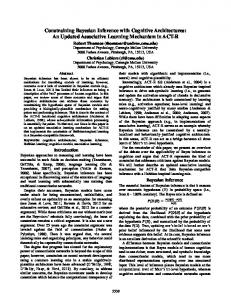
2. Description of Procedure The proposed procedure uses the Bayesian reliability inference to determine system (or unit) reliability and failure distribution, to support the optimisation of maintenance strategies, and so forth. The general procedure begins with the collection of reliability data (see Figure 1). These are the observed values of a physical process, such as various “lifetime data.”

2

Journal of Quality and Reliability Engineering Action

(11) Data updating and inference improvement

Plan

History information

Current data set

(10) Inference making

(1) Data preparation

Reliability data, and so forth

Prior knowledge

(2) Priors’ inspection and integration

Posterior results

Study

(3) Prior selection

Bayesian model average

Do

MCMC model average

(4) Model selection

(9) Model comparison

(5) Posterior sampling

No (6) MCMC convergence diagnostic

Yes

(7) Monte Carlo error diagnostic

(8) Model improvement

Accept

No

Figure 1: An integrated procedure for Bayesian reliability inference via MCMC.

The data may be subject to uncertainties, such as imprecise measurement, censoring, truncated information, and interpretation errors. Reliability data are found in the “current data set”; they contain original data and include the evaluation, manipulation, and/or organisation of data samples. At a higher level in the collection of data, a wide variety of “historical information” can be obtained, including the results of inspecting and integrating this “information,” thereby adding to “prior knowledge.” The final level is reliability inference, which is the process of making a conclusion based on “posterior results.” Using the definitions shown in Figure 1, we propose an integrated procedure which constructs a full framework for the standardized process of Bayesian reliability inference. As shown in Figure 1, the procedure is composed of a continuous improvement process including four stages (Plan, Do, Study, and Action) which will be discussed later in this section and 11 sequential steps: (1) data preparation; (2) prior inspection and integration; (3) prior selection; (4) model selection; (5) posterior sampling; (6) MCMC convergence diagnostic; (7) Monte Carlo error diagnostic; (8) model improvement; (9)

model comparison; (10) inference making; (11) data updating and inference improvement. Step 1 (data preparation). The original data sets for “history information” and “current data” related to reliability studies need to be acquired, evaluated, and merged. In this way, “history information” can be transferred to “prior knowledge,” and “current data” can become “reliability data” in later steps. Step 2 (prior inspection and integration). During this step, “prior knowledge” receives a second and more extensive treatment, including a reliability consistency check, a credence test, and a multisource integration. This step improves prior reliability data. Step 3 (prior selection). This step uses the results achieved in Step 2 to determine the model’s form and parameters, for instance, selecting informative or noninformative priors, or unknown parameters and their distributed forms. Step 4 (model selection). This step determines a reliability model (parametric or nonparametric), selecting from 𝑛

Journal of Quality and Reliability Engineering candidates for the studied system/units. It considers both “reliability data” and the inspection, integration, and selection of priors to implement the 𝑖th (𝑖 = 1, . . . , 𝑖 + 1, . . . , 𝑛). Step 5 (posterior sampling). In this step, we determine a sampling method (e.g., Gibbs sampling, Metropolis-Hastings sampling, etc.) to implement MCMC simulation for the model’s posterior calculations. Step 6 (MCMC convergence diagnostic). In this step, we check whether the Markov chains have reached convergence. If they have, we move on to the next step; if they have not, we return to Step 5 and redetermine the iteration times of posterior sampling or rechoose the sampling methods; if the results still cannot be satisfied, we return to Steps 3 and 4 and redetermine the prior selection and model selection. Step 7 (Monte Carlo error diagnostic). We need to decide if the Monte Carlo error is small enough to be accepted in this step. As discussed in Step 6, if it is accepted, we go on to the next step; if it is not, we return to Step 5 and redecide the iteration times of the posterior sampling or rechoose the sampling methods; if the results still cannot be accepted, we go back to Steps 3 and 4 and recalculate the prior selection and model selection. Step 8 (model improvement). Here, we choose the 𝑖 + 1th candidate model and restart from Step 4. Step 9 (model comparison). After implementing 𝑛 candidate models, we need to (1) compare the posterior results to determine the most suitable model or (2) adopt the average posterior estimations (using the Bayesian model average or the MCMC model average) as the final results. Step 10 (inference making). After achieving the posterior results in Step 9, we can perform Bayesian reliability inference to determine system (or unit) reliability, find the failure distribution, optimise maintenance strategies, and so forth. Step 11 (data updating and inference improvement). Along with the passage of time, new “current data” can be obtained, relegating “previous” inference results to “historical data.” By updating “reliability data” and “prior knowledge,” and restarting at Step 1, we can improve the reliability inference. In summary, by using this step-by-step method, we can create a continuous improvement process for the Bayesian reliability inference. Note that Steps 1, 2, and 3 are assigned to the “Plan” stage when data for MCMC implementation are prepared. In addition, a part of Steps 1, 2, and 3 refers to the elicitation of prior knowledge. Steps 4 and 5 are both assigned to the “Do” stage, where the MCMC sampling is carried out. Steps 6 to 9 are treated as the “Study” stage; in these steps, the sampling results are checked and compared; in addition, knowledge is accumulated and improved upon by implementing various candidate reliability models. The “Action” stage consists of Steps 10 and 11; at this point, a continuously improved loop can be obtained. In other words, by implementing the

3 step-by-step procedure, we can accumulate and gradually update prior knowledge. Equally, posterior results will be improved upon and become increasingly robust, thereby improving the accuracy of the inference results. Also note that this paper will focus on six steps and their relationship to MCMC inference implementation: (1) prior elicitation; (2) model construction; (3) posterior sampling; (4) MCMC convergence diagnostic; (5) Monte Carlo error diagnostic; (6) model comparison.

3. Elicitation of Prior Knowledge In the proposed procedure, the elicitation of prior knowledge plays a crucial role. It is related to Steps 1, 2, and 3 and is part of the Plan Stage, as shown in Figure 1. In practice, prior information is derived from a variety of data sources and is also considered “historical data” (or “experience data”). Those data taking various forms require various processing methods. Although in the first step, “historical information” can be transferred to “prior knowledge,” this is not enough. Credible prior information and proper forms of these data are necessary to compute the model’s posterior probabilities, especially in the case of a small sample set. Meanwhile, either noncredible or improper prior data may cause instability in the estimation of the model’s probabilities or lead to convergence problems in MCMC implementation. This section will discuss some relevant prior elicitation problems in Bayesian reliability inference, namely, including acquiring priors, performing a consistency check and credence test, fusing multisource priors, and selecting which priors to use in MCMC implementation. 3.1. Acquisition of Prior Knowledge. In Bayesian reliability analysis, prior knowledge comes from a wide range of historical information. As shown in Figure 2, data sources include (1) engineering design data; (2) component test data; (3) system test data; (4) operational data from similar systems; (5) field data in various environments; (6) computer simulations; (7) related standards and operation manuals; (8) experience data from similar systems; (9) expert judgment and personal experience. Of these, the first seven yield objective prior data, and the last two provide subjective prior data. Prior data also take a variety of forms, including reliability data, the distribution of reliability parameters, moments, confidence intervals, quantiles, and upper and lower limits. 3.2. Inspection of Priors. In Bayesian analysis, different prior information will lead to similar results when the data sample is sufficiently large. While the selection of priors and their form has little influence on posterior inferences, in practice, particularly with a small data sample, we know that some prior information is associated with the current observed reliability data. However, we are not sure whether the prior distributions are the same as the posterior distributions. In other words, we cannot confirm that all posterior distributions converge and are consistent (a consistency check issue). Even if they pass a consistency check, we can only say that they are consistent under a certain specified confidence interval. Therefore, an important prerequisite for applying any

4

Journal of Quality and Reliability Engineering Information

Knowledge

Engineering design

Reliability data

Component test

Operational data from similar systems Field data under various environments

Parameters’ distributions Objective

Systems test

Parameters’ moments Transfer

Parameters’ confidence intervals

Computer simulations Parameters’ quantiles

Experience data from similar systems Expert judgment and personal experience from studied system

Subjective

Related standards and operation manual

Parameters’ upper limits Parameters’ lower limits

Figure 2: Data source: transfer from historical to prior knowledge.

prior information is to confirm its credibility by performing a consistency check and credence test. As noted by Li [25], the consistency check of prior and posterior distributions was first studied from a statistical viewpoint by Walker [26]. Under specified conditions, posterior distributions are not only consistent with those of the priors, but they have an asymptotic normality which could simplify their calculation. Li [25] also notes that studies on the consistency check of priors have focused on checking the moments and confidence intervals of reliability parameters, as well as historical data. A number of checking methodologies have been developed, including robustness analysis, significance test, Smirnov test, rank-sum test, and mood test. More studies have been reviewed by Ghosal [27] and Choi et al. [28]. The credibility of prior information can be viewed as the probability that it and the collected data come from the same population. Li [25] lists the following methods to perform a credence test: frequency method, bootstrap method, ranksum text, and so forth. However, in the case of a small sample or simulated data, the above methods are not suitable because even if data pass the credence test, selecting different priors will lead to different results. We therefore suggest a comprehensive use of the above methods to ensure the superiority of Bayesian inference. 3.3. Fusion of Prior Information. Due to the complexity of the system, not to mention the diversification of test equipment and methodologies, prior information can come from many sources. As all priors can pass a consistency check, an integrated fusion estimation based on the smoothness of credibility is sometimes necessary. In such situations, a common choice is parallel fusion estimation or serial fusion estimation, achieved by determining the reliability parameters’ weighted credibility [25]. However, as the credibility computation can be difficult, other methods to fuse the priors may be called for. In the area of reliability, related research studies include the following. Savchuk and Martz [29] develop Bayes

estimators for the true binomial survival probability when there are multiple sources of prior information; Ren et al. [30] adopt Kullback information as the distance measure between different prior information and fusion distributions, minimizing the sum to get the combined prior distribution; looking at aerospace propulsion as a case study, Liu et al. [31] discuss a similar fusion problem in a complex system and suggest [32] a fusion approach based on expert experience with the analytic hierarchy process (AHP); Fang [33] proposes using multisource information fusion techniques with Fuzzy-Bayesian for reliability assessment; Zhou et al. [34] propose a Bayes fusion approach for assessment of spaceflight products, integrating degradation data and field lifetime data with Fisher information and the Weiner process. In general, the most important thing for multisource integration is to determine the weights of the different priors. 3.4. Selection of Priors Based on MCMC. In Bayesian reliability inference, two kinds of priors are very useful: the conjugate prior and the noninformative prior. To apply MCMC methods, however, the “log-concave prior” is recommended. The conjugate prior family is very popular because it is convenient for mathematical calculation. The concept, along with the term “conjugate prior,” was introduced by Howard and Robert [35] in their work on Bayesian decision theory. If the posterior distributions are in the same family as the prior distributions, the prior and posterior distributions are called conjugate distributions, and the prior is called a conjugate prior. For instance, the Gaussian family is a conjugate of itself (or a self-conjugate) with respect to a Gaussian likelihood function: if the likelihood function is Gaussian, choosing a Gaussian prior distribution over the mean distribution will ensure that the posterior distribution is also Gaussian. This means that the Gaussian distribution is a conjugate prior for the likelihood function which is also Gaussian. Other examples include the following: the conjugate distribution of a normal distribution is a normal or inverse-normal distribution; the Poisson and the exponential distribution’s

Journal of Quality and Reliability Engineering conjugate both have a Gamma distribution, while the Gamma distribution is a self-conjugate; the binomial and the negative binomial distribution’s conjugate both have a Beta distribution; the polynomial distribution’s conjugate is a Dirichlet distribution. Noninformative prior refers to a prior for which we only know certain parameters’ value ranges or their importance; for example, there may be a uniform distribution. A noninformative prior can also be called a vague prior, flat prior, diffuse prior, ignorance prior, and so forth. There are many different ways to determine the distribution of a noninformative prior, including Bayes hypothesis, Jeffrey’s rule, reference prior, inverse reference prior, probability-matching prior, maximum entropy prior, relative likelihood approach, cumulative distribution function, Monte Carlo method, bootstrap method, random weighting simulation method, Haar invariant measurement, Laplace prior, Lindley rule, generalized maximum entropy principle, and the use of marginal distributions. From another perspective, the types of prior distribution also include informative prior, hierarchical prior, Power prior, and nonparameter prior processes. At this point, there are no set rules for selecting prior distributions. Regardless of the manner used to determine a prior’s distribution, the selected prior should be both reasonable and convenient for calculation. Of the above, the conjugate prior is a common choice. To facilitate the calculation of MCMC, especially for adaptive rejection sampling and Gibbs sampling, a popular choice is log-concave prior distribution. Log-concave prior distribution refers to a prior distribution in which the natural logarithm is concave; that is, the second derivative is nonpositive. Common logarithmic concavity prior distributions include the normal distribution family, logistic distribution, Student’s-𝑡 distribution, the exponential distribution family, the uniform distribution on a finite interval greater than the gamma distribution with a shape parameter greater than 1, and Beta distribution with a value interval (0, 1). As logarithmic concavity prior distributions are very flexible, this paper recommends their use in reliability studies.

4. Model Construction To apply MCMC methods, we divide the reliability models into four categories: parametric, semiparametric, frailty, and other nontraditional reliability models. Parametric modelling offers straightforward modelling and analysis techniques. Common choices include Bayesian exponential model, Bayesian Weibull model, Bayesian extreme value model, Bayesian log-normal model, and Gamma model. Lin et al. [36] present a reliability study using the Bayesian parametric framework to explore the impact of a railway train wheel’s installed position on its service lifetime and to predict its reliability characteristics. They apply a MCMC computational scheme to obtain the parameters’ posterior distributions. Besides the hierarchical reliability models mentioned above, other parametric models include Bayesian accelerated failure models (AFM), Bayesian reliability growth models, and Bayesian faulty tree analysis (FTA).

5 Semiparametric reliability models have become quite common and are well accepted in practice, since they offer a more general modelling strategy with fewer assumptions. In these models, the failure rate is described in a semiparametric form, or the priors are developed by a stochastic process. With respect to the semiparametric failure rate, Lin and Asplund [37] adopt the piecewise constant hazard model to analyze the distribution of the locomotive wheels’ lifetime. The applied hazard function is sometimes called a piecewise exponential model; it is convenient because it can accommodate various shapes of the baseline hazard over a number of intervals. In a study of the processes of priors, Ibrahim et al. [38] examine the gamma process, beta process, correlated prior processes, and the Dirichlet process separately, using an MCMC computational scheme. By introducing the gamma process of the prior’s increment, Lin et al. [39] propose its reliability when applied to the Gibbs sampling scheme. In reliability inference, most studies are implemented under the assumption that individual lifetimes are independent and identically distributed (i.i.d.). However, Cox proportional hazard (CPH) models can sometimes not be used because of the dependence of data within a group. Take train wheels as an example because they have the same operating conditions, the wheels mounted on a particular locomotive may be dependent. In a different context, some data may come from multiple records of wheels installed in the same position but on other locomotives. Modelling dependence has received considerable attention, especially in cases where the datasets may come from related subjects of the same group [40, 41]. A key development in modelling such data is to build frailty models in which the data are conditionally independent. When frailties are considered, the dependence within subgroups can be considered an unknown and unobservable risk factor (or explanatory variable) of the hazard function. In a recent reliability study, Lin and Asplund [37] consider a gamma shared frailty to explore the unobserved covariates’ influence on the wheels on the same locomotive. Some nontraditional Bayesian reliability models are both interesting and helpful. For instance, Lin et al. [10] point out that in traditional methods of reliability analysis, a complex system is often considered to be composed of several subsystems in series. The failure of any subsystem is usually considered to lead to the failure of the entire system. However, some subsystems’ lifetimes are long enough or they never fail during the life cycle of the entire system. In addition, such subsystems’ lifetimes will not be influenced equally under different circumstances. For example, the lifetimes of some screws will far exceed the lifetime of the compressor in which they are placed. However, the failure of the compressor’s gears may directly lead to its failure. In practice, such interferences will affect the model’s accuracy, but are seldom considered in traditional analysis. To address these shortcomings, Lin et al. [10] present a new approach to reliability analysis for complex systems, in which a certain fraction of subsystems is defined as a “cure fraction” based on the consideration that such subsystems’ lifetimes are long enough or they never fail during the life cycle of the entire system; this is called the cure rate model.

6

Journal of Quality and Reliability Engineering

5. Posterior Sampling To implement MCMC calculations, Markov chains require a stationary distribution. There are many ways to construct these chains. During the last decade, the following Monte Carlo (MC) based sampling methods for evaluating highdimensional posterior integrals have been developed: MC importance sampling, Metropolis-Hastings sampling, Gibbs sampling, and other hybrid algorithms. In this section, we introduce two common samplings: (1) Metropolis-Hastings sampling, the best known MCMC sampling algorithm, and (2) Gibbs sampling, the most popular MCMC sampling algorithm in the Bayesian computation literature, which is actually a special case of Metropolis-Hastings sampling. 5.1. Metropolis-Hastings Sampling. Metropolis-Hastings sampling is a well-known MCMC sampling algorithm, which comes from importance sampling. It was first developed by Metropolis et al. [42] and later generalized by Hastings [43]. Tierney [44] gives a comprehensive theoretical exposition of the algorithm; Chib and Greenberg [45] provide an excellent tutorial on it. Suppose that we need to create a sample using the probability density function 𝑝(𝜃). Let 𝐾 be a regular constant; this is a complicated calculation (e.g., a regular factor in Bayesian analysis) and is normally an unknown parameter. Then, let 𝑝(𝜃) = ℎ(𝜃)/𝐾. Metropolis sampling from 𝑝(𝜃) can be described as follows. Step 1. Choose an arbitrary starting point 𝜃0 , and set ℎ(𝜃0 ) > 0.

from 𝜃𝑡 to 𝜃𝑡+1 is related to 𝜃𝑡 but not related to 𝜃0 , 𝜃1 , . . . , 𝜃𝑡−1 . After experiencing a sufficiently long burn-in period, the Markov chain reaches a steady state and the sampling points 𝜃𝑡+1 , . . . , 𝜃𝑡+𝑛 from 𝑝(𝜃) are obtained. Metropolis-Hastings sampling was promoted by Hastings [43]. The candidate generating distribution can adopt any form and does not need to be symmetric. In MetropolisHastings sampling, the acceptance probability 𝛼 can be written as 𝛼 (𝜃𝑡−1 , 𝜃∗ ) = min (1,

ℎ (𝜃∗ ) 𝑞 (𝜃∗ , 𝜃𝑡−1 ) ). ℎ (𝜃𝑡−1 ) 𝑞 (𝜃𝑡−1 , 𝜃∗ )

(3)

In the above equation, as 𝑞(𝜃∗ , 𝜃𝑡−1 ) = 𝑞(𝜃𝑡−1 , 𝜃∗ ), and Metropolis-Hastings sampling becomes Metropolis sampling. The Markov transfer probability function can therefore be ∗ { {𝑞 (𝜃𝑡−1 , 𝜃 ) ℎ (𝜃∗ ) 𝑝 (𝜃, 𝜃 ) = { {𝑞 (𝜃𝑡−1 , 𝜃∗ ) ℎ (𝜃𝑡−1 ) { ∗

ℎ (𝜃∗ ) > ℎ (𝜃𝑡−1 ) ℎ (𝜃∗ ) < ℎ (𝜃𝑡−1 ) .

(4)

From another perspective, when using Metropolis-Hastings sampling, say we need to generate the candidate point 𝜃∗ . In this case, generate an arbitrary 𝜇 from a uniform distribution 𝑈(0, 1). Set 𝜃𝑡 = 𝜃∗ if 𝜇 ≤ 𝛼 (𝜃𝑡−1 , 𝜃∗ ) and 𝜃𝑡 = 𝜃𝑡−1 otherwise.

(2)

5.2. Gibbs Sampling. Metropolis-Hastings sampling is convenient for lower-dimensional numerical computation. However, if 𝜃 has a higher dimension, it is not easy to choose an appropriate candidate generating distribution. By using Gibbs sampling, we only need to know the full conditional distribution. Therefore, it is more advantageous in high-dimensional numerical computation. Gibbs sampling is essentially a special case of Metropolis-Hastings sampling, as the acceptance probability equals one. It is currently the most popular MCMC sampling algorithm in the Bayesian reliability inference literature. Gibbs sampling is based on the ideas of Grenander [46], but the formal term comes from S. Geman and D. Geman [47] to analyze lattice in image processing. A landmark work for Gibbs sampling in problems of Bayesian inference is Gelfand and Smith [48]. Gibbs sampling is also called heat bath algorithm in statistical physics. A similar idea, data augmentation, is introduced by Tanner and Wong [49]. Gibbs sampling belongs to the Markov update mechanism and adopts the ideology of “divide and conquer.” It supposes that all other parameters are fixed and known, inferring a set of parameters. Let 𝜃𝑖 be a random parameter or several parameters in the same group. For the 𝑗th group, the conditional distribution is 𝑓(𝜃𝑗 ). To carry out Gibbs sampling, the basic scheme is as follows.

Following the above steps, generate a Markov chain with the sampling points 𝜃0 , 𝜃1 , . . . , 𝜃𝑘 , . . . . The transfer probability

Step 1. Choose an arbitrary starting point 𝜃(0) = (𝜃1(0) , . . . , 𝜃𝑘(0) ).

Step 2. Generate a proposal distribution 𝑞(𝜃1 , 𝜃2 ), which represents the probability for 𝜃2 to be the next transfer value as the current value is 𝜃1 . The distribution 𝑞(𝜃1 , 𝜃2 ) is named as the candidate generating distribution. This candidate generating distribution is symmetric, which means that 𝑞(𝜃1 , 𝜃2 ) = 𝑞(𝜃2 , 𝜃1 ). Now based on the current 𝜃, generate a candidate point 𝜃∗ from 𝑞(𝜃1 , 𝜃2 ). Step 3. For the specified candidate point 𝜃∗ , calculate the density ratio 𝛼 with 𝜃∗ and the current value 𝜃𝑡−1 as follows: 𝛼 (𝜃𝑡−1 , 𝜃∗ ) =

𝑝 (𝜃∗ ) ℎ (𝜃∗ ) = . 𝑝 (𝜃𝑡−1 ) ℎ (𝜃𝑡−1 )

(1)

The ratio 𝛼 refers to the probability to accept 𝜃∗ , where the constant 𝐾 can be neglected. Step 4. If 𝜃∗ increases the probability density, so that 𝛼 > 1, then accept 𝜃∗ and let 𝜃𝑡 = 𝜃∗ . Otherwise, if 𝛼 < 1, then let 𝜃𝑡 = 𝜃𝑡−1 and go to Step 2. The acceptance probability 𝛼 can be written as 𝛼 (𝜃𝑡−1 , 𝜃∗ ) = min (1,

ℎ (𝜃∗ ) ). ℎ (𝜃𝑡−1 )


7

Step 2. Generate 𝜃1(1) from the conditional distribution 𝑓(𝜃1 | 𝜃2(0) , . . . , 𝜃𝑘(0) ) and generate 𝜃2(1) from the conditional distribution 𝑓(𝜃2 | 𝜃1(1) , 𝜃3(0) , . . . , 𝜃𝑘(0) ). (1) (0) Step 3. Generate 𝜃𝑗(1) from 𝑓(𝜃𝑗 | 𝜃1(1) , . . . , 𝜃𝑗−1 , 𝜃𝑗+1 , . . . , 𝜃𝑘(0) ). (1) Step 4. Generate 𝜃𝑘(1) from 𝑓(𝜃𝑘 | 𝜃1(1) , 𝜃2(1) , . . . , 𝜃𝑘−1 ).

As shown above, one-step transitions from 𝜃(0) to 𝜃(1) =

(𝜃1(1) , . . . , 𝜃𝑘(1) ), where 𝜃(1) can be viewed as a one-time accom-

plishment of the Markov chain. Step 5. Go back to Step 2.

After 𝑡 iterations, 𝜃(𝑡) = (𝜃1(𝑡) , . . . , 𝜃𝑘(𝑡) ) can be obtained, and each component 𝜃(1) , 𝜃(2) , 𝜃(3) , . . . will be achieved. The Markov transition probability function is 𝑝 (𝜃, 𝜃∗ ) = 𝑓 (𝜃1 | 𝜃2 , . . . , 𝜃𝑘 ) 𝑓 (𝜃2 | 𝜃1∗ , 𝜃3 , . . . , 𝜃𝑘 ) ⋅ ⋅ ⋅

(5)

∗ ). 𝑓 (𝜃𝑘 | 𝜃1∗ , . . . , 𝜃𝑘−1

Starting from different 𝜃(0) , as 𝑡 → ∞, the marginal distribution of 𝜃(𝑡) can be viewed as a stationary distribution based on the theory of the ergodic average. In this case, the Markov chain is seen as converging and the sampling points are seen as observations of the sample. For both methods, it is not necessary to choose the candidate generating distribution, but it is necessary to do sampling from the conditional distribution. There are many other ways to do sampling from the conditional distribution, including sample-importance resampling, rejection sampling, and adaptive rejection sampling (ARS).

6. Markov Chain Monte Carlo Convergence Diagnostic Because of the Markov chain’s ergodic property, all statistics inferences are implemented under the assumption that the Markov chain converges. Therefore, the Markov Chain Monte Carlo convergence diagnostic is very important. When applying MCMC for reliability inference, if the iteration times are too small, the Markov chain will not “forget” the influence of the initial values; if the iteration times are simply increased to a large number, there will be insufficient scientific evidence to support the results, causing a waste of resources. Markov chain Monte Carlo convergence diagnostic is a hot topic for Bayesian researchers. Efforts to determine MCMC convergence have been concentrated in two areas. The first is theoretical, and the second is practical. For the former, the Markov transition kernel of the chain is analyzed in an attempt to predetermine a number of iterations that will insure convergence in a total variation distance within a specified tolerance of the true stationary distribution. Related studies include Polson [50], Roberts and Rosenthal [51], and Mengersen and Tweedie [52]. While approaches like these are

promising, they typically involve sophisticated mathematics, as well as laborious calculations that must be repeated for every model under consideration. As for practical studies, most research is focused on developing diagnostic tools, including Gelman and Rubin [53], Raftery and Lewis [54], Garren and Smith [55], and Roberts and Rosenthal [56]. When these tools are used, sometimes the bounds obtained are quite loose; even so, they are considered both reasonable and feasible. At this point, more than 15 MCMC convergence diagnostic tools have been developed. In addition to a basic tool which provides intuitive judgments by tracing a time series plot of the Markov chain, other examples include tools developed by Gelman and Rubin [53], Raftery and Lewis [54], Garren and Smith [55], Brooks and Gelman [57], Geweke [58], Johnson [59], Mykland et al. [60], Ritter and Tanner [61], Roberts [62], Yu [63], Yu and Mykland [64], Zellner and Min [65], Heidelberger and Welch [66], and Liu et al. [67]. We can divide diagnostic tools into categories depending on the following: (1) if the target distribution needs to be monitored; (2) if the target distribution needs to calculate a single Markov chain or multiple chains; (3) if the diagnostic results depend on the output of the Monte Carlo algorithm, not on other information from the target distribution. It is not wise to rely on one convergence diagnostic technique, and researchers suggest a more comprehensive use of different diagnostic techniques. Some suggestions include (1) simultaneously diagnosing the convergence of a set of parallel Markov chains; (2) monitoring the parameters’ autocorrelations and cross-correlations; (3) changing the parameters of the model or the sampling methods; (4) using different diagnostic methods and choosing the largest preiteration times as the formal iteration times; (5) combining the results obtained from the diagnostic indicators’ graphs. Six tools have been achieved by computer programs. The most widely used are the convergence diagnostic tools proposed by Gelman and Rubin [53] and Raftery and Lewis [54]; the latter is an extension of the former. Both are based on the theory of analysis of variance (ANOVA); both use multiple Markov chains and both use the output to perform the diagnostic. 6.1. Gelman-Rubin Diagnostic. In traditional literature on iterative simulations, many researchers suggest that to guarantee the Markov chain’s diagnostic ability, multiple parallel chains should be used simultaneously to do the iterative simulation for one target distribution. In this case, after running the simulation for a certain period, it is necessary to determine whether the chains have “forgotten” the initial value and if they converge. Gelman and Rubin [53] point out that lack of convergence can sometimes be determined from multiple independent sequences but cannot be diagnosed using simulation output from any single sequence. They also find that more information can be obtained during one single Markov chain’s replication process than in multiple chains’ iterations. Moreover, if the initial values are more dispersed, the status of nonconvergence is more easily found. Therefore, they propose a method using multiple replications of the chain to decide whether it becomes stationary in the second

8


half of each sample path. The idea behind this is an implicit assumption that convergence will be achieved within the first half of each sample path; the validity of this assumption is tested by the Gelman-Rubin diagnostic or the variance ratio method. Based on normal theory approximations to exact Bayesian posterior inference, Gelman-Rubin diagnostic involves two steps. In Step 1, for a target scalar summary 𝜑, select an overdispersed starting point from its target distribution 𝜋(𝜑). Then, generate 𝑚 Markov chains for 𝜋(𝜑), where each chain has 2𝑛 times iterations. Delete the first 𝑛 times iterations and use the second 𝑛 times iterations for analysis. In Step 2, apply the between-sequence variance 𝐵/𝑛 and the within-sequence variance 𝑊 to compare the corrected scale reduction factor (CSRF). CSRF is calculated by 𝑚 Markov chains and the formed 𝑚𝑛 values in the sequences which stem from 𝜋(𝜑). By comparing the CSRF value, the convergence diagnostic can be implemented. In addition, 2 1 𝑚 𝐵 = ∑ (𝜑𝑗. − 𝜑.. ) , 𝑛 𝑚 − 1 𝑗=1

𝜑𝑗. =

1 𝑛 ∑𝜑 , 𝑛 𝑡=1 𝑗𝑡

𝑊=

𝑚 𝑛 2 1 ∑ ∑ (𝜑𝑗𝑡 − 𝜑𝑗. ) , 𝑚 (𝑛 − 1) 𝑗=1 𝑡=1

𝜑.. =

1 𝑚 ∑𝜑 , 𝑚 𝑗=1 𝑗.

(6)

where 𝜑𝑗𝑡 denotes the 𝑡th of the 𝑛 iterations of 𝜑 in chain 𝑗 and 𝑗 = 1, . . . , 𝑚, 𝑡 = 1, . . . , 𝑛. Let 𝜑 be a random variable of 𝜋(𝜑), with mean 𝜇 and variance 𝜎2 under the target distribution. ̂ To explain Suppose that 𝜇̂ has some unbiased estimator 𝑉. ̂ the variability between 𝜇̂ and 𝑉, Gelman and Rubin construct ̂ as Student’s 𝑡-distribution with a mean 𝜇̂ and variance 𝑉 follows: ̂ = 𝑛 − 1 𝑊 + (1 + 1 ) 𝐵 , (7) 𝜇̂ = 𝜑.. , 𝑉 𝑛 𝑚 𝑛 ̂ is a weighted average of 𝑊 and 𝐵. The above where 𝑉 estimation will be unbiased if the starting points of the sequences are drawn from the target distribution. However, it will be overestimated if the starting distribution is overdiŝ is also called a “conservative” estimate. persed. Therefore, 𝑉 Meanwhile, because the iteration number 𝑛 is limited, the within-sequence variance 𝑊 can be too low, leading to falsely ̂ and 𝑊 should diagnosing convergence. As 𝑛 → ∞, both 𝑉 2 be close to 𝜎 . In other words, the scale of current distribution of 𝜑 should be decreasing as 𝑛 is increasing. ̂ 𝑠 = √̂ 𝑉/𝜎2 as the scale reduction factor (SRF). Denote √𝑅 ̂ 𝑝 = √̂ 𝑉/𝑊 becomes the potential scale By applying 𝑊, √𝑅 reduction factor (PSRF). By applying a correct factor df/(df − 2) for PSRF, a correct scale reduction factor (CSRF) can be obtained as follows: ̂ ̂ 𝑐 = √ ( 𝑉 ) df = √ ( 𝑛 − 1 + 𝑚 + 1 𝐵 ) df , √𝑅 𝑊 df − 2 𝑛 𝑚𝑛 𝑊 df − 2 (8)

where df represents the degree of freedom in Student’s 𝑡̂ Var(𝑉). ̂ The distribution. Following Fisher [68], df ≈ 2𝑉/ diagnostic based on CSRF can be implemented as follows: ̂ 𝑐 > 1, it indicates that the iteration number 𝑛 is too if 𝑅 ̂ will become smaller and 𝑊 small. When 𝑛 is increasing, 𝑉 ̂ 𝑐 is close to 1 (e.g., 𝑅 ̂ 𝑐 < 1.2), we can will become larger. If 𝑅 conclude that each of the 𝑚 sets of 𝑛 simulated observations is close to the target distribution, and the Markov chain can be viewed as converging. 6.2. Brooks-Gelman Diagnostic. Although the Gelman-Rubin diagnostic is very popular, its theory has several defects. Therefore, Brooks and Gelman [57] extend the method in the following way. First, in the above equation, df/(df − 2) represents the ratio of the variance between the Student 𝑡-distribution and the normal distribution. Brooks and Gelman [57] point out some obvious defects in the equation. For instance, if the convergence speed is slow, or df < 2, CSRF could be infinite and may even be negative. Therefore, they set up a new and correct factor for PSRF; the new CSRF becomes ̂ ∗ = √ ( 𝑛 − 1 + 𝑚 + 1 𝐵 ) df + 3 . √𝑅 𝑐 𝑛 𝑚𝑛 𝑊 df + 1

(9)

Second, Brooks and Gelman [57] propose a new and more easily implemented way to calculate PSRF. The first step is similar to Gelman-Rubin’s diagnostic. Using 𝑚 chains’ second 𝑛 iterations, obtain an empirical interval 100(1 − 𝛼%) after each chain’s second 𝑛 iteration. Then, 𝑚 empirical intervals can be achieved within a sequence, denoted by 𝑙. In the second step, determine the total empirical intervals for sequences from 𝑚𝑛 estimates of 𝑚 chains, denoted by 𝐿. Finally, calculate the PSRF as follows: ̂∗ = √ 𝑙 . √𝑅 𝑝 𝐿

(10)

The basic theory behind the Gelman-Rubin and BrooksGelman diagnostics is the same. The difference is that we compare the variance in the former and the interval length in the latter. Third, Brooks and Gelman [57] point out that the value of CSRF being close to one is a necessary but not sufficient condition for MCMC convergence. Additional condition is ̂ should stabilize as a function of 𝑛. That that both 𝑊 and 𝑉 ̂ have not reached the steady state, is to say, if 𝑊 and 𝑉 CSRF could still be one. In other words, before convergence, ̂ and both should be close to one. Therefore, as 𝑊 < 𝑉 an alternative, Brooks and Gelman [57] propose a graphical approach to monitoring convergence. Divide the 𝑚 sequences ̂ ̂ 𝑐 (𝑘) into batches of length 𝑏. Then calculate 𝑉(𝑘), 𝑊(𝑘), and 𝑅 based upon the latter half of the observations of a sequence of ̂ ̂ 𝑐 (𝑘) √𝑊(𝑘), and 𝑅 length 2𝑘𝑏, for 𝑘 = 1, . . . , 𝑛/𝑏. Plot √𝑉(𝑘), as a function of 𝑘 on the same plot. Approximate convergence ̂ 𝑐 (𝑘) is close to one and at the same time, both is attained if 𝑅 ̂ 𝑉(𝑘) and 𝑊(𝑘) stabilize at one.


9

Fourth and finally, Brooks and Gelman [57] discuss the multivariate situation. Let 𝜑 denote the parameter vector and calculate the following:

𝜌̂𝑘 =

𝑚

󸀠 𝐵 1 = ∑ (𝜑𝑗. − 𝜑.. ) (𝜑𝑗. − 𝜑.. ) , 𝑛 𝑚 − 1 𝑗=1

(11)

Let 𝜆 1 be maximum characteristic root of 𝑊−1 𝐵/𝑛; then, the PSRF can be expressed as 𝑛−1 𝑚+1 + 𝜆 . 𝑛 𝑚 1

(12)

7. Monte Carlo Error Diagnostic When implementing the MCMC method, besides determining the Markov chains’ convergence diagnostic, we must check two uncertainties related to the Monte Carlo point estimation: statistical uncertainty and Monte Carlo uncertainty. Statistical uncertainty is determined by the sample data and the adopted model. Once the data are given and the models are selected, the statistical uncertainty is fixed. For maximum likelihood estimation (MLE), statistical uncertainty can be calculated by the inverse square root of the Fisher information. For Bayesian inference, statistical uncertainty is measured by the parameters’ posterior standard deviation. Monte Carlo uncertainty stems from the approximation of the model’s characteristics, which can be measured by a suitable standard error (SE). Monte Carlo standard error of the mean, also called Monte Carlo error (MC error), is a wellknown diagnostic tool. In this case, define MC error as the ratio of the sample’s standard deviation and the square root of the sample volume, which can be written as SE [𝐼̂ (𝑦)] =

𝑛−𝑘 Cov (𝜃𝑡 , 𝜃𝑡+𝑘 ) ∑𝑡=1 (𝜃𝑡 − 𝜃) (𝜃𝑡−𝑘 − 𝜃) , = 2 Var (𝜃𝑡 ) ∑𝑛−𝑘 (𝜃 − 𝜃) 𝑡=1

𝑚 𝑛 󸀠 1 𝑊= ∑ ∑ (𝜑𝑗𝑡 − 𝜑𝑗. ) (𝜑𝑗𝑡 − 𝜑𝑗. ) . 𝑚 (𝑛 − 1) 𝑗=1 𝑡=1

√𝑅𝑝 = √

𝜌(𝜃𝑖 , 𝜃𝑖+𝑘 ) ≠ 0. Then, the autocorrelation coefficient 𝜌𝑘 can be calculated by

SD [𝐼̂ (𝑦)] √𝑛 2

1/2

1 1 𝑛 =[ ( ∑ (ℎ (𝑦 | 𝑥𝑖 )) − 𝐼̂ (𝑦)) ] 𝑛 𝑛 − 1 𝑖=1 [ ]

. (13)

Obviously, as 𝑛 becomes larger, MC error will be smaller. Meanwhile, the average of the sample data will be closer to the average of the population. As in the MCMC algorithm, we cannot guarantee that all the sampled points are independent and identically distributed (i.i.d.); we must correct the sequence’s correlation. To this end, we introduce the autocorrelation function and sample size inflation factor (SSIF). Following the sampling methods introduced in Section 5, define a sampling sequence 𝜃1 , . . . , 𝜃𝑛 with length 𝑛. Suppose there are autocorrelations which exist among the adjacent sampling points; this means that 𝜌(𝜃𝑖 , 𝜃𝑖+1 ) ≠ 0. Furthermore,

(14)

𝑡

where 𝜃 = 1/𝑛 ∑𝑛𝑡=1 𝜃𝑡 . Following the above discussion, the MC error with consideration of autocorrelations in MCMC implementation can be written as SE (𝜃) =

SD 1 + 𝜌 √ . √𝑛 1 − 𝜌

(15)

In the above equation, SD/√𝑛 represents the MC error ̂ shown in SE[𝐼(𝑦)]. Meanwhile, √(1 + 𝜌)/(1 − 𝜌) represents the SSIF. SD/√𝑛 is helpful to determine whether the sample volume 𝑛 is sufficient, and SSIF reveals the influence of the autocorrelations on the sample data’s standard deviation. Therefore, by following each parameter’s MC error, we can evaluate the accuracy of its posterior. The core idea of the Monte Carlo method is to view the integration of some function 𝑓(𝑥) as an expectation of the random variable; therefore, the sampling methods implemented on the random variable are very important. If the sampling distribution is closer to 𝑓(𝑥), the MC error will be smaller. In other words, by increasing the sample volume or improving the adopted models, the statistical uncertainty could be reduced; the improved sampling methods could also reduce the Monte Carlo uncertainty.

8. Model Comparison In Step 8, we might have several candidate models which could pass the MCMC convergence diagnostic and the MC error diagnostic. Thus, model comparison is a crucial part of reliability inference. Broadly speaking, discussions of the comparison of Bayesian models focus on Bayes factors, model diagnostic statistics, measure of fit, and so forth. In a more narrow sense, the concept of model comparison refers to selecting a better model after comparing several candidate models. The purpose of doing model comparison is not to determine the model’s correctness. Rather, it is to find out why some models are better than others (e.g., which parametric model or non-parametric model; which prior distribution; which covariates; which family of parameters for application, etc.) or to obtain an average estimation based on the weighted estimate of the model parameters and stemming from the posterior probability of model comparison (e.g., model average). In Bayesian reliability inference, the model comparison methods can be divided into three categories: (1) separate estimation [69–82] including posterior predictive distribution, Bayes factors (BF) and its approximate estimation-Bayesian information criterion (BIC), deviance information criterion (DIC), pseudoBayes factor (PBF), and conditional predictive ordinate (CPO). It also includes some estimations based

10

Journal of Quality and Reliability Engineering on the likelihood theory, using the same as BF but offering more flexibility, for instance, harmonic mean estimator, importance sampling, reciprocal importance estimator, bridge sampling, candidate estimator, Laplace-Metropolis estimator, data augmentation estimator, and so forth;

Suppose there are two models, 𝑀1 and 𝑀2 . Let BF12 denote the Bayes factors, equal to the ratio of the posterior odds of the models to the prior odds:

(2) comparative estimation including different distance measures [83–87]: entropy distance, Kullback-Leibler divergence (KLD), 𝐿-measure, and weighted 𝐿-measure;

The above equation shows that BF12 equals the ratio of the model likelihoods for the two models. Thus, it can be written as

(3) simultaneous estimation [49, 88–92] including reversible Jump MCMC (RJMCMC), birth-and-death MCMC (BDMCMC), and fusion MCMC (FMCMC).

(19)

Related reference reviews are given by Kass and Raftery [70], Tatiana et al. [91], and Chen and Huang [93]. This section introduces three popular comparison methods used in Bayesian reliability studies: BF, BIC, and DIC. BF is the most traditional method, BIC is BF’s approximate estimation, and DIC improves BIC by dealing with the problem of the parameters’ degree of freedom. 8.1. Bayes Factors (BF). Suppose that 𝑀 represents 𝑘 models which need to be compared. The data set 𝐷 stems from 𝑀𝑖 (𝑖 = 1, . . . , 𝑘), and 𝑀1 , . . . , 𝑀𝑘 are called competing models. Let 𝑓(𝐷 | 𝜃𝑖 , 𝑀𝑖 ) = 𝐿(𝜃𝑖 | 𝐷, 𝑀𝑖 ) denote the distribution of 𝐷, with consideration of the 𝑖th model and its unknown parameter vector 𝜃 of dimension 𝑝𝑖 , also called the likelihood function of 𝐷 with a specified model. Under prior distribution 𝜋(𝜃𝑖 | 𝑀𝑖 ) and ∑𝑘𝑖=1 𝜋(𝜃𝑖 | 𝑀𝑖 ) = 1, the marginal distributions of 𝐷 are found by integrating out the parameters as follows: 𝑝 (𝐷 | 𝑀𝑖 ) = ∫ 𝑓 (𝐷 | 𝜃𝑖 , 𝑀𝑖 ) 𝜋 (𝜃𝑖 | 𝑀𝑖 ) 𝑑𝜃𝑖 ,

(16)

Θ𝑖

where Θ𝑖 represents the parameter data set for the 𝑖th mode. As in the data likelihood function, the quantity 𝑝(𝐷 | 𝑀𝑖 ) = 𝐿(𝐷 | 𝑀𝑖 ) is called model likelihood. Suppose we have some preliminary knowledge about model probabilities 𝜋(𝑀𝑖 ); after considering the given observed data set 𝐷, the posterior probability of 𝑖th model being the best model is determined as

=

𝑝 (𝐷 | 𝑀𝑖 ) 𝜋 (𝑀𝑖 ) 𝑝 (𝐷) 𝜋 (𝑀𝑖 ) ∫ 𝑓 (𝐷 | 𝜃𝑖 , 𝑀𝑖 ) 𝜋 (𝜃𝑖 | 𝑀𝑖 ) 𝑑𝜃𝑖 ∑𝑘𝑗=1

[𝜋 (𝑀𝑗 ) ∫ 𝑓 (𝐷 | 𝜃𝑗 , 𝑀𝑗 ) 𝜋 (𝜃𝑗 | 𝑀𝑗 ) 𝑑𝜃𝑗 ]

𝑝 (𝑀1 | 𝐷) 𝜋 (𝑀2 ) 𝑝 (𝐷 | 𝑀1 ) × = . 𝑝 (𝑀2 | 𝐷) 𝜋 (𝑀1 ) 𝑝 (𝐷 | 𝑀2 )

𝑝 (𝑀1 | 𝐷) 𝑝 (𝐷 | 𝑀1 ) 𝜋 (𝑀1 ) = × . 𝑝 (𝑀2 | 𝐷) 𝑝 (𝐷 | 𝑀2 ) 𝜋 (𝑀2 )

(18)

We can also say that BF12 shows the ratio of posterior odds of the model 𝑀1 and the prior odds of 𝑀1 . In this way, the collection of model likelihoods 𝑝(𝐷 | 𝑀𝑖 ) is equivalent to the model probabilities themselves (since the prior probabilities 𝜋(𝑀𝑖 ) are known in advance) and, hence, could be considered as the key quantities needed for Bayesian model choice. Jeffreys [94] recommends a scale of evidence for interpreting Bayes factors. Kass and Raftery [70] provide a similar scale, along with a complete review of Bayes factors, including their interpretation, computation or approximation, and robustness to the model-specific prior distributions and applications in a variety of scientific problems. 8.2. Bayesian Information Criterion (BIC). Under some situations, it is difficult to calculate BF, especially for those models which consider different random effects, or adopt diffusion priors or a large number of unknown and informative priors. Therefore, we need to calculate BF’s approximate estimation. The Bayesian information criterion (BIC) is also called the Schwarz information criterion (SIC) and is the most important method to get BF’s approximate estimation. The key point of BIC is to obtain the approximate estimation of 𝑝(𝐷 | 𝑀𝑖 ). It is proved by Volinsky and Raftery [72] that ln 𝑝 (𝐷 | 𝑀𝑖 ) ≈ ln 𝑓 (𝐷 | 𝜃̂𝑖 , 𝑀𝑖 ) −

𝑝𝑖 ln (𝑛) . 2

(20)

Then, we get SIC as follows: ln BF12 = ln 𝑝 (𝐷 | 𝑀1 ) − ln 𝑝 (𝐷 | 𝑀2 ) 𝑝 − 𝑝2 = ln 𝑓 (𝐷 | 𝜃̂1 , 𝑀1 ) − ln 𝑓 (𝐷 | 𝜃̂2 , 𝑀2 ) − 1 ln (𝑛) . 2 (21)

𝑝 (𝑀𝑖 | 𝐷) =

BF12 =

As discussed above, considering two models, 𝑀1 and 𝑀2 , BIC12 represents the likelihood ratio test statistic with model sample size 𝑛 and the model’s complexity as penalty. It can be written as

. (17)

The integration part of the above equation is also called the prior predictive density or marginal likelihood, where 𝑝(𝐷) is a nonconditional marginal likelihood of 𝐷.

BIC12 = −2 ln BF12 = −2 ln (

(22) 𝑓 (𝐷 | 𝜃̂1 , 𝑀1 ) ) + (𝑝1 − 𝑝2 ) ln (𝑛) , 𝑓 (𝐷 | 𝜃̂ , 𝑀 ) 2

2


11

Locomotive

Right

I 1

Axels 1, 2, 3

Bogies I, II

I 2

Right

I

II 1

3

3

Left

Left

(a)

II

II 2

(b)

Figure 3: Locomotive wheels’ installation positions.

where 𝑝𝑖 is proportional to the model’s sample size and complexity. Kass and Raftery [70] discuss BIC’s calculation program. Kass and Wasserman [73] show how to decide 𝑛. Volinsky and Raftery [72] discuss the way to choose 𝑛 if the data are censored. If 𝑛 is large enough, BF’s approximate estimation can be written as

9. Discussions with a Case Study In this section, we discuss a case study for a locomotive wheel’s degradation data to illustrate the proposed procedure. The case was first discussed by Lin et al. [36].

(26)

9.1. Background. The service life of a railway wheel can be significantly reduced due to failure or damage, leading to excessive cost and accelerated deterioration. This case study focuses on the wheels of the locomotive of a cargo train. While two types of locomotives with the same type of wheels are used in cargo trains, we consider only one. There are two bogies for each locomotive and three axels for each bogie (Figure 3). The installed position of the wheels on a particular locomotive is specified by a bogie number (I, II—number of bogies on the locomotive), an axel number (1, 2, 3—number of axels for each bogie) and the side of the wheel on the alxe (right or left) where each wheel is mounted. The diameter of a new locomotive wheel in the studied railway company is 1250 mm. In the company’s current maintenance strategy, a wheel’s diameter is measured after running a certain distance. If it is reduced to 1150 mm, the wheel is replaced by a new one. Otherwise, it is reprofiled or other maintenance strategies are implemented. A threshold level for failure is defined as 100 mm (= 1250 mm – 1150 mm). The wheel’s failure condition is assumed to be reached if the diameter reaches 100 mm. The company’s complete database also includes the diameters of all locomotive wheels at a given observation time, the total running distances corresponding to their “time to be maintained,” and the wheels’ bill of material (BOM) data, from which we can determine their positions. Two assumptions are made: (1) for each censored datum it is supposed that the wheel is replaced; (2) degradation is linear. Only one locomotive is considered in this example to ensure that (1) all wheel’s maintenance strategies are the same; (2) the alxe load and running speed are obviously constant; and (3) the operational environments including routes, climates, and exposure are common for all wheels. The data set contains 46 datum points (𝑛 = 46) of a single locomotive throughout the period November 2010 to January 2012. We take the following steps to obtain locomotive wheels’ lifetime data (see Figure 4).

Select the model with a lower DIC value. As DIC < 5, the difference between models can be ignored.

(i) Establish a threshold level 𝐿 𝑠 , where 𝐿 𝑠 = 100 mm (1250 mm – 1150 mm).

BF12 ≈ exp (−0.5BIC12 ) .

(23)

Obviously, if the BIC is smaller, we should consider model 𝑀1 ; otherwise, 𝑀2 should be considered. 8.3. Deviance Information Criterion (DIC). Traditional methods for model comparison consider two main aspects: the model’s measure of fit and the model’s complexity. Normally, the model’s measure of fit can be increased by increasing the model’s complexity. For this reason, most model comparison methods are committed balancing both two points. To utilize BIC, the number 𝑝 of free parameters of the model must be calculated. However, for complex Bayesian hierarchical models, it is very difficult to get 𝑝’s exact number. Therefore, Spiegelhalter et al. [74] propose the deviance information criterion (DIC) to compare Bayesian models. Celeux et al. [95] discuss DIC issues for a censored data set; this paper and other researchers’ discussion of it are representative literature in the DIC field in recent years. DIC utilizes deviance to evaluate the model’s measure of fit, and it utilizes the number of parameters to evaluate its complexity. Note that it is consistent with the Akaike information criterion (AIC), which is used to compare classical models [96]. Let 𝐷(𝜃) denote the Bayesian deviance, and 𝐷 (𝜃) = −2 log (𝑝 (𝐷 | 𝜃)) .

(24)

Let 𝑝𝑑 denote the model’s effective number of parameters, and 𝑝𝑑 = 𝐷 (𝜃) − 𝐷 (𝜃) = − ∫ 2 ln (𝑝 (𝐷 | 𝜃)) 𝑑𝜃 − (−2 ln (𝑝 (𝐷 | 𝜃))) .

(25)

Then, DIC = 𝐷 (𝜃) + 2𝑝𝑑 = 𝐷 (𝜃) + 𝑝𝑑 .

12


Degradation (mm)

100

B2 B1

Ls

9.3. Do. In the Do Stage, we set up the three models noted above for the degradation analysis: Bayesian exponential regression model, Bayesian Weibull regression model, and Bayesian log-normal regression model. For our calculations, we implement Gibbs sampling. The joint likelihood function for the exponential regression model, Weibull regression model, and log-normal regression model is given as follows (Lin et al. [36]):

L1 L2

0

𝛽 ∼ 𝑁(0, 0.0001); for lognormal regression: 𝜏 ∼ 𝐺(1, 0.01), 𝛽 ∼ 𝑁(0, 0.0001).

D1

D2

Distance (km)

Figure 4: Plot of the wheel degradation data: one example.

(i) exponential regression model: 𝑛

𝜐𝑖

𝐿 (𝛽 | 𝐷) = ∏[exp (xi󸀠 𝛽) exp (− exp (xi󸀠 𝛽) 𝑡𝑖 )] 𝑖=1

× [exp (− exp (xi󸀠 𝛽) 𝑡𝑖 )]

(ii) Transfer observed 90 records of wheel diameters at reported time 𝑡 degradation data; this equals to 1250 mm minus the corresponding observed diameter. (iii) Assume a liner degradation path and construct a degradation line 𝐿 𝑖 (e.g., 𝐿 1 , 𝐿 2 ) using the origin point and the degradation data (e.g., 𝐵1 , 𝐵2 ). (iv) Set 𝐿 𝑠 = 𝐿 𝑖 , get the point of intersection and the corresponding lifetimes data (e.g., 𝐷1 , 𝐷2 ). To explore the impact of a locomotive wheel’s installed position on its service lifetime and to predict its reliability characteristics, the Bayesian exponential regression model, Bayesian Weibull regression model, and Bayesian log-normal regression model are used to establish the wheel’s lifetime using degradation data and taking into account the position of the wheel. For each reported datum, a wheel’s installation position is documented, and as mentioned above, positioning is used in this study as a covariate. The wheel’s position (bogie, axel, and side) or covariate X is denoted by 𝑥1 (bogie I: 𝑥1 = 1, bogie II: 𝑥1 = 2), 𝑥2 (axel 1: 𝑥2 = 1, axel 2: 𝑥2 = 2, and axel 3, 𝑥2 = 3), and 𝑥3 (right: 𝑥3 = 1, left: 𝑥3 = 2). Correspondingly, the covariates’ coefficients are represented by 𝛽1 , 𝛽2 , and 𝛽3 . In addition, 𝛽0 is defined as random effect. The goal is to determine reliability, failure distribution, and optimal maintenance strategies for the wheel. 9.2. Plan. During the Plan Stage, we first collect the “current data,” as mentioned in Section 9.1, including the diameter measurements of the locomotive wheel, total distances corresponding to the “time to maintenance,” and the wheel’s bill of material (BOM) data. Then, see Figure 4, we note the installed position and transfer the diameter into degradation data, which becomes “reliability data” during the “data preparation” process. We consider the noninformative prior for the constructed models and select the vague prior with log-concave form, which has been determined to be a suitable choice as a noninformative prior selection. For exponential regression: 𝛽 ∼ 𝑁(0, 0.0001); for Weibull regression: 𝛼 ∼ 𝐺(0.2, 0.2),

1−𝜐𝑖

𝑛

𝑛

𝑖=1

𝑖=1

= exp [∑ 𝜐𝑖 xi󸀠 𝛽] exp [− ∑ exp (xi󸀠 𝛽) 𝑡𝑖 ] ; (27) (ii) Weibull regression model: 𝐿 (𝛼, 𝛽 | 𝐷) 𝑛

𝑛

= 𝛼∑𝑖=1 𝜐𝑖 exp {∑𝜐𝑖 [xi󸀠 𝛽 + 𝜐𝑖 (𝛼 − 1) ln (𝑡𝑖 ) 𝑖=1

(28)

− exp (xi󸀠 𝛽) 𝑡𝑖𝛼 ] } ; (iii) log-normal regression model: 𝐿 (𝛽, 𝜏 | 𝐷) −(1/2) ∑𝑛𝑖=1 𝜐𝑖

= (2𝜋𝜏−1 )

×

𝑛

−𝜐 ∏𝑡𝑖 𝑖 {1 𝑖=1

2 𝜏 𝑛 exp {− ∑ 𝜐𝑖 [(ln (𝑡𝑖 ) − xi󸀠 𝛽)] } 2 𝑖=1 1−𝜐𝑖

ln (𝑡𝑖 ) − xi󸀠 𝛽 − Φ[ ]} 𝜏−1/2

. (29)

9.4. Study. After checking the MCMC convergence diagnostic and accepting the Monte Carlo error diagnostic for all three models, in the Study Stage, we compare the model with the three DIC values. After comparing the DIC values, we select the Bayesian log-normal regression model as the most suitable one (see Table 1). Accordingly, the locomotive wheels’ reliability functions are achieved: (i) exponential regression model: 𝑅 (𝑡𝑖 | X) = exp [− exp (−5.862 − 0.072𝑥1 −0.032𝑥2 − 0.012𝑥3 ) × 𝑡𝑖 ] ; (30)


13

10. Conclusions

Table 1: DIC summaries. 𝐷(𝜃) 648.98 472.22 442.03

Model Exponential Weibull Log-normal

𝐷(𝜃) 645.03 467.39 436.87

𝑝𝑑 3.95 4.83 5.16

DIC 652.93 477.05 447.19

Table 2: MTTF statistics based on Bayesian log-normal regression model. Bogie

Axel 1 (𝑥2 = 1)

I (𝑥1 = 1) 2 (𝑥2 = 2) 3 (𝑥2 = 3) 1 (𝑥2 = 1) II (𝑥1 = 2) 2 (𝑥2 = 2) 3 (𝑥2 = 3)

Side Right (𝑥3 = 1) Left (𝑥3 = 2) Right (𝑥3 = 1) Left (𝑥3 = 2) Right (𝑥3 = 1) Left (𝑥3 = 2) Right (𝑥3 = 1) Left (𝑥3 = 2) Right (𝑥3 = 1) Left (𝑥3 = 2) Right (𝑥3 = 1) Left (𝑥3 = 2)

𝜇𝑖 MTTF (×103 km) 5.9532 387.03 5.9543 387.46 5.9740 395.16 5.9751 395.60 5.9947 403.43 5.9958 403.87 6.0205 413.97 6.0216 414.43 6.0413 422.67 6.0424 423.14 6.0621 431.56 6.0632 432.03

This paper has proposed an integrated procedure for Bayesian reliability inference using Markov chain Monte Carlo methods. The goal is to build a full framework for related academic research and engineering applications to implement modern computational-based Bayesian approaches, especially for reliability inference. The suggested procedure is a continuous improvement process with four stages (Plan, Do, Study, and Action) and 11 sequential steps including (1) data preparation; (2) priors’ inspection and integration; (3) prior selection; (4) model selection; (5) posterior sampling; (6) MCMC convergence diagnostic; (7) Monte Carlo error diagnostic; (8) model improvement; (9) model comparison; (10) inference making; (11) data updating and inference improvement. The paper illustrates the proposed procedure using a case study. It concludes that the procedure can be used to perform Bayesian reliability inference to determine system (or unit) reliability, failure distribution and to support maintenance strategies optimization, and so forth.

Conflict of Interests The authors declare that there is no conflict of interests regarding the publication of this paper.

Acknowledgments

(ii) Weibull regression model: 𝑅 (𝑡𝑖 | X) = exp ⌊ − exp (−60.47 − 0.078𝑥1 −0.146𝑥2 − 0.050𝑥3 ) × 𝑡𝑖10.08 ⌋ ; (31)

The author would like to thank Lule˚a Railway Research Centre (Järnvägstekniskt Centrum, Sweden) for initiating the research study and Swedish Transport Administration (Trafikverket) for providing financial support.

References (iii) log-normal regression model: 𝑅 (𝑡𝑖 | X) = 1 − Φ[

ln (𝑡𝑖 ) − (5.864 + 0.067𝑥1 + 0.02𝑥2 + 0.001𝑥3 ) (187.5)−1/2

].

(32)

9.5. Action. With the chosen model’s posterior results, in the Action Stage, we make our maintenance predictions (Table 2) and apply them to the proposed maintenance inspection level. This, in turn, allows us to evaluate and optimise the wheel’s replacement and maintenance strategies (including the reprofiling interval, inspection interval, and lubrication interval). As more data are collected in the future, the old “current data set” will be replaced by new “current data”; meanwhile, the results achieved in this case will become “history information,” which will be transferred to be “prior knowledge” and a new cycle will start. With this step-by-step method, we can create a continuous improvement process for the locomotive wheel’s reliability inference.

[1] D. L. Kelly and C. L. Smith, “Bayesian inference in probabilistic risk assessment—the current state of the art,” Reliability Engineering and System Safety, vol. 94, no. 2, pp. 628–643, 2009. [2] P. Congdon, Bayesian Statistical Modeling, John Wiley & Sons, Chichester, UK, 2001. [3] P. Congdon, Applied Bayesian Modeling, John Wiley & Sons, Chichester, UK, 2003. [4] D. G. Robinson, “A hierarchical bayes approach to system reliability analysis,” Tech. Rep. Sandia 2001-3513, Sandia National Laboratories, 2001. [5] V. E. Johnson, “A hierarchical model for estimating the reliability of complex systems,” in Bayesian Statistics 7, J. M. Bernardo, Ed., Oxford University Press, Oxford, UK, 2003. [6] A. G. Wilson, “Hierarchical Markov Chain Monte Carlo (MCMC) for bayesian system reliability,” Encyclopedia of Statistics in Quality and Reliability, 2008. [7] J. Lin, M. Asplund, and A. Parida, “Bayesian parametric analysis for reliability study of locomotive wheels,” in Proceedings of the 59th Annual Reliability and Maintainability Symposium (RAMS ’13), Orlando, Fla, USA, 2013. [8] G. Tont¸, L. Vlˇadˇareanu, M. S. Munteanu, and D. G. Tont¸, “Hierarchical Bayesian reliability analysis of complex dynamical systems,” in Proceedings of the 9th WSEAS International Conference on Applications of Electrical Engineering (AEE ’10), pp. 181– 186, March 2010.

14 [9] J. Lin, “A two-stage failure model for Bayesian change point analysis,” IEEE Transactions on Reliability, vol. 57, no. 2, pp. 388– 393, 2008. [10] J. Lin, M. L. Nordenvaad, and H. Zhu, “Bayesian survival analysis in reliability for complex system with a cure fraction,” International Journal of Performability Engineering, vol. 7, no. 2, pp. 109–120, 2011. [11] M. Hamada, H. F. Martz, C. S. Reese, T. Graves, V. Johnson, and A. G. Wilson, “A fully Bayesian approach for combining multilevel failure information in fault tree quantification and optimal follow-on resource allocation,” Reliability Engineering and System Safety, vol. 86, no. 3, pp. 297–305, 2004. [12] T. L. Graves, M. S. Hamada, R. Klamann, A. Koehler, and H. F. Martz, “A fully Bayesian approach for combining multi-level information in multi-state fault tree quantification,” Reliability Engineering and System Safety, vol. 92, no. 10, pp. 1476–1483, 2007. [13] L. Kuo and B. Mallick, “Bayesian semiparametric inference for the accelerated failure-time model,” The Canadian Journal of Statistics, vol. 25, no. 4, pp. 457–472, 1997. [14] S. Walker and B. K. Mallick, “A Bayesian semiparametric accelerated failure time model,” Biometrics, vol. 55, no. 2, pp. 477–483, 1999. [15] T. Hanson and W. O. Johnson, “A Bayesian semiparametric AFT model for interval-censored data,” Journal of Computational and Graphical Statistics, vol. 13, no. 2, pp. 341–361, 2004. [16] S. K. Ghosh and S. Ghosal, “Semiparametric accelerated failure time models for censored data,” in Bayesian Statistics and Its Applications, S. K. Upadhyay, Ed., Anamaya Publishers, New Delhi, India, 2006. [17] A. Komárek and E. Lesaffre, “The regression analysis of correlated interval-censored data: illustration using accelerated failure time models with flexible distributional assumptions,” Statistical Modelling, vol. 9, no. 4, pp. 299–319, 2009. [18] G. Y. Li, Q. G. Wu, and Y. H. Zhao, “On bayesian analysis of binomial reliability growth,” The Japan Statistical Society, vol. 32, no. 1, pp. 1–14, 2002. [19] J. Y. Tao, Z. M. Ming, and X. Chen, “The bayesian reliability growth models based on a new dirichlet prior distribution,” in Reliability, Risk and Safety, C. G. Soares, Ed., Chapter 237, CRC Press, 2009. [20] L. Kuo and T. Y. Yang, “Bayesian reliability modeling for masked system lifetime data,” Statistics and Probability Letters, vol. 47, no. 3, pp. 229–241, 2000. [21] K. Ilkka, “Methods and problems of software reliability estimation,” Tech. Rep. VTT Working Papers 1459-7683, VTT Technical Research Centre of Finland, 2006. [22] Y. Tamura, H. Takehara, and S. Yamada, “Component-oriented reliability analysis based on hierarchical bayesian model for an open source software,” American Journal of Operations Research, vol. 1, pp. 25–32, 2011. [23] G. I. Schuëller and H. J. Pradlwarter, “Benchmark study on reliability estimation in higher dimensions of structural systems— an overview,” Structural Safety, vol. 29, no. 3, pp. 167–182, 2007. [24] S. K. Au, J. Ching, and J. L. Beck, “Application of subset simulation methods to reliability benchmark problems,” Structural Safety, vol. 29, no. 3, pp. 183–193, 2007. [25] R. Li, Bayes reliability studies for complex system [Doctor thesis], National University of Defense Technology, 1999, Chinese. [26] A. M. Walker, “On the asymptotic behavior of posterior distributions,” Journal of Royal Statistics Society B, vol. 31, no. 1, pp. 80–88, 1969.

Journal of Quality and Reliability Engineering [27] S. Ghosal, “A review of consistency and convergence of posterior distribution. Technical report,” in Proceedings of National Conference in Bayesian Analysis, Benaras Hindu University, Varanashi, India, 2000. [28] T. Choi, R. V. B. C. Ramamoorthi, and S. Ghosal, Eds., Pushing the Limits of Contemporary Statistics: Contributions in Honor of Jayanta K. Ghosh, Institute of Mathematical Statistics, Beachwood, Ohio, USA, 2008. [29] V. P. Savchuk and H. F. Martz, “Bayes reliability estimation using multiple sources of prior information: binomial sampling,” IEEE Transactions on Reliability, vol. 43, no. 1, pp. 138–144, 1994. [30] K. J. Ren, M. D. Wu, and Q. Liu, “The combination of prior distributions based on kullback information,” Journal of the Academy of Equipment of Command & Technology, vol. 13, no. 4, pp. 90–92, 2002. [31] Q. Liu, J. Feng, and J.-L. Zhou, “Application of similar system reliability information to complex system Bayesian reliability evaluation,” Journal of Aerospace Power, vol. 19, no. 1, pp. 7–10, 2004. [32] Q. Liu, J. Feng, and J. Zhou, “The fusion method for prior distribution based on expert’s information,” Chinese Space Science and Technology, vol. 24, no. 3, pp. 68–71, 2004. [33] G. H. Fang, Research on the multi-source information fusion techniques in the process of reliability assessment [Doctor thesis], Hefei University of Technology, China, 2006. [34] Z. B. Zhou, H. T. Li, X. M. Liu, G. Jin, and J. L. Zhou, “A bayes information fusion approach for reliability modeling and assessment of spaceflight long life product,” Journal of Systems Engineering, vol. 32, no. 11, pp. 2517–2522, 2012. [35] R. Howard and S. Robert, Applied Statistical Decision Theory, Division of Research, Graduate School of Business Administration, Harvard University, 1961. [36] J. Lin, M. Asplund, and A. Parida, “Reliability analysis for degradation of locomotive wheels using parametric bayesian approach,” Quality and Reliability Engineering International, 2013. [37] J. Lin and M. Asplund, “Bayesian semi-parametric analysis for locomotive wheel degradation using gamma frailties,” Journal of Rail and Rapid Transit, 2013. [38] J. G. Ibrahim, M. H. Chen, and D. Sinha, Bayesian Survival Analysis, 2001. [39] J. Lin, Y.-Q. Han, and H.-M. Zhu, “A semi-parametric proportional hazards regression model based on gamma process priors and its application in reliability,” Chinese Journal of System Simulation, vol. 22, pp. 5099–5102, 2007. [40] S. K. Sahu, D. K. Dey, H. Aslanidou, and D. Sinha, “A weibull regression model with gamma frailties for multivariate survival data,” Lifetime Data Analysis, vol. 3, no. 2, pp. 123–137, 1997. [41] H. Aslanidou, D. K. Dey, and D. Sinha, “Bayesian analysis of multivariate survival data using Monte Carlo methods,” Canadian Journal of Statistics, vol. 26, no. 1, pp. 33–48, 1998. [42] N. Metropolis, A. W. Rosenbluth, M. N. Rosenbluth, A. H. Teller, and E. Teller, “Equation of state calculations by fast computing machines,” The Journal of Chemical Physics, vol. 21, no. 6, pp. 1087–1092, 1953. [43] W. K. Hastings, “Monte carlo sampling methods using Markov chains and their applications,” Biometrika, vol. 57, no. 1, pp. 97– 109, 1970. [44] L. Tierney, “Markov chains for exploring posterior distributions,” The Annals of Statistics, vol. 22, no. 4, pp. 1701–1762, 1994.

Journal of Quality and Reliability Engineering [45] S. Chib and E. Greenberg, “Understanding the metropolishastings algorithm,” Journal of American Statistician, vol. 49, pp. 327–335, 1995. [46] U. Grenander, Tutorial in Pattern Theory, Division of Applied Mathematics, Brow University, Providence, RI, USA, 1983. [47] S. Geman and D. Geman, “Stochastic relaxation, Gibbs distributions and the Bayesian restoration of images,” IEEE Transactions on Pattern Analysis and Machine Intelligence, vol. 6, no. 6, pp. 721–741, 1984. [48] A. E. Gelfand and A. F. M. Smith, “Sampling-based approaches to calculation marginal densities,” Journal of American Asscioation, vol. 85, pp. 398–409, 1990. [49] M. A. Tanner and W. H. Wong, “The calculation of posterior distributions by data augmentation (with discussion),” Journal of American Statistical Association, vol. 82, pp. 805–811, 1987. [50] N. G. Polson, “Convergence of markov chain conte carlo algorithms,” in Bayesian Statistics 5, Oxford University Press, Oxford, UK, 1996. [51] G. O. Roberts and J. S. Rosenthal, “Markov-chain Monte Carlo: some practical implications of theoretical results,” Canadian Journal of Statistics, vol. 26, no. 1, pp. 4–31, 1997. [52] K. L. Mengersen and R. L. Tweedie, “Rates of convergence of the Hastings and Metropolis algorithms,” The Annals of Statistics, vol. 24, no. 1, pp. 101–121, 1996. [53] A. Gelman and D. B. Rubin, “Inference from iterative simulation using multiple sequences (with discussion),” Statistical Science, vol. 7, pp. 457–511, 1992. [54] A. E. Raftery and S. Lewis, “How many iterations in the gibbs sampler,” in Bayesian Statistics 4, pp. 763–773, Oxford University Press, Oxford, UK, 1992. [55] S. T. Garren and R. L. Smith, Convergence Diagnostics for Markov Chain Samplers, Department of Statistics, University of North Carolina, 1993. [56] G. O. Roberts and J. S. Rosenthal, “Markov-chain Monte Carlo: some practical implications of theoretical results,” Canadian Journal of Statistics, vol. 26, no. 1, pp. 5–31, 1998. [57] S. P. Brooks and A. Gelman, “General methods for monitoring convergence of iterative simulations,” Journal of Computational and Graphical Statistics, vol. 7, no. 4, pp. 434–455, 1998. [58] J. Geweke, “Evaluating the accuracy of sampling-based approaches to the calculation of posterior moments,” in Bayesian Statistics 4, J. M. Bernardo, J. Berger, A. P. Dawid, and A. F. M. Smith, Eds., pp. 169–193, Oxford University Press, Oxford, UK, 1992. [59] V. E. Johnson, “Studying convergence of markov chain monte carlo algorithms using coupled sampling paths,” Tech. Rep., Institute for Statistics and Decision Sciences, Duke University, 1994. [60] P. Mykland, L. Tierney, and B. Yu, “Regeneration in markov chain samplers,” Journal of the American Statistical Association, no. 90, pp. 233–241, 1995. [61] C. Ritter and M. A. Tanner, “Facilitating the gibbs sampler: the gibbs stopper and the griddy gibbs sampler,” Journal of the American Statistical Association, vol. 87, pp. 861–868, 1992. [62] G. O. Roberts, “Convergence diagnostics of the gibbs sampler,” in Bayesian Statistics 4, pp. 775–782, Oxford University Press, Oxford, UK, 1992. [63] B. Yu, Monitoring the Convergence of Markov Samplers Based on Estimated L1 Error, Department of Statistics, University of California, Berkeley, Calif, USA, 1994.

15 [64] B. Yu and P. Mykland, Looking at Markov Samplers through Cusum Path Plots: A Simple Diagnostic Idea, Department of Statistics, University of California, Berkeley, Calif, USA, 1994. [65] A. Zellner and C. K. Min, “Gibbs sampler convergence criteria,” Journal of the American Statistical Association, vol. 90, pp. 921– 927, 1995. [66] P. Heidelberger and P. D. Welch, “Simulation run length control in the presence of an initial transient,” Operations Research, vol. 31, no. 6, pp. 1109–1144, 1983. [67] C. Liu, J. Liu, and D. B. Rubin, “A variational control variable for assessing the convergence of the gibbs sampler,” in Proceedings of the American Statistical Association, Statistical Computing Section, pp. 74–78, 1992. [68] J. F. Lawless, Statistical Models and Method for Lifetime Data, John Wiley & Sons, New York, NY, USA, 1982. [69] A. Gelman, J. B. Carlin, H. S. Stern, and D. B. Rubin, Bayesian Data Analysis, Chapman and Hall/CRC Press, New York, NY, USA, 2004. [70] R. A. Kass and A. E. Raftery, “Bayes factor,” Journal of American Stattistical Association, vol. 90, pp. 773–795, 1995. [71] A. Gelfand and D. Dey, “Bayesian model choice: asymptotic and exact calculations,” Journal of Royal Statistical Society B, vol. 56, pp. 501–514, 1994. [72] C. T. Volinsky and A. E. Raftery, “Bayesian information criterion for censored survival models,” Biometrics, vol. 56, no. 1, pp. 256– 262, 2000. [73] R. E. Kass and L. Wasserman, “A reference bayesian test for nested hypotheses and its relationship to the schwarz criterion,” Journal of American Statistical Association, vol. 90, pp. 928–934, 1995. [74] D. J. Spiegelhalter, N. G. Best, B. P. Carlin, and A. van der Linde, “Bayesian measures of model complexity and fit,” Journal of the Royal Statistical Society B, vol. 64, no. 4, pp. 583–639, 2002. [75] S. Geisser and W. Eddy, “A predictive approach to model selection,” Journal of American Statistical Association, vol. 74, pp. 153–160, 1979. [76] A. E. Gelfand, D. K. Dey, and H. Chang, “Model determinating using predictive distributions with implementation via sampling-based methods (with discussion),” in Bayesian Statistics 4, Oxford University Press, Oxford, UK, 1992. [77] M. Newton and A. Raftery, “Approximate bayesian inference by the weighted likelihood bootstrap,” Journal of Royal Statistical Society B, vol. 56, pp. 1–48, 1994. [78] P. J. Lenk and W. S. Desarbo, “Bayesian inference for finite mixtures of generalized linear models with random effects,” Psychometrika, vol. 65, no. 1, pp. 93–119, 2000. [79] X.-L. Meng and W. H. Wong, “Simulating ratios of normalizing constants via a simple identity: a theoretical exploration,” Statistica Sinica, vol. 6, no. 4, pp. 831–860, 1996. [80] S. Chib, “Marginal likelihood from the Gibbs output,” Journal of the American Statistical Association, vol. 90, pp. 1313–1321, 1995. [81] S. Chib and I. Jeliazkov, “Marginal likelihood from the metropolis-hastings output,” Journal of the American Statistical Association, vol. 96, no. 453, pp. 270–281, 2001. [82] S. M. Lewis and A. E. Raftery, “Estimating Bayes factors via posterior simulation with the Laplace-Metropolis estimator,” Journal of the American Statistical Association, vol. 92, no. 438, pp. 648–655, 1997. [83] S. K. Sahu and R. C. H. Cheng, “A fast distance-based approach for determining the number of components in mixtures,” Canadian Journal of Statistics, vol. 31, no. 1, pp. 3–22, 2003.

16 [84] K. Mengersen and C. P. Robert, “Testing for mixtures: a bayesian entropic approach,” in Bayesian Statistics 5, Oxford University Press, Oxford, UK, 1996. [85] J. G. Ibrahim and P. W. Laud, “A predictive approach to the analysis of designed experiments,” Journal of the American Statistical Association, vol. 89, pp. 309–319, 1994. [86] A. E. Gelfand and S. K. Ghosh, “Model choice: a minimum posterior predictive loss approach,” Biometrika, vol. 85, no. 1, pp. 1–11, 1998. [87] M.-H. Chen, D. K. Dey, and J. G. Ibrahim, “Bayesian criterion based model assessment for categorical data,” Biometrika, vol. 91, no. 1, pp. 45–63, 2004. [88] P. J. Green, “Reversible jump Markov chain monte carlo computation and Bayesian model determination,” Biometrika, vol. 82, no. 4, pp. 711–732, 1995. [89] C. Robert and G. Casella, Monte Carlo Statistical Methods, Springer, New York, NY, USA, 2004. [90] M. Stephens, “Bayesian analysis of mixture models with an unknown number of components—an alternative to reversible jump methods,” Annals of Statistics, vol. 28, no. 1, pp. 40–74, 2000. [91] M. Tatiana, F. S. Sylvia, and D. A. Georg, Comparison of Bayesian Model Selection Based on MCMC with an Application to GARCH-Type Models, Vienna University of Economics and Business Administration, 2003. [92] P. C. Gregory, “Extra-solar planets via Bayesian fusion MCMC,” in Astrostatistical Challenges for the New Astronomy, J. M. Hilbe, Ed., Springer Series in Astrostatistics, Chapter 7, Springer, New York, NY, USA, 2012. [93] H. Chen and S. Huang, “A comparative study on model selection and multiple model fusion,” in Proceedings of the 7th International Conference on Information Fusion (FUSION ’05), pp. 820–826, July 2005. [94] H. Jeffreys, Theory of Probability, Oxford Univiersity Press, Oxford, UK, 1961. [95] G. Celeux, F. Forbes, C. P. Robert, and D. M. Titterington, “Deviance information criteria for missing data models,” Bayesian Analysis, vol. 1, no. 4, pp. 651–674, 2006. [96] H. Akaike, “Information theory and an extension of the maximum likelihood principle,” in Proceedings of the 2nd International Symposium on Information Theory, Tsahkadsor, 1971.


International Journal of

Rotating Machinery

The Scientific World Journal Hindawi Publishing Corporation http://www.hindawi.com

Volume 2014

Journal of

Robotics Hindawi Publishing Corporation http://www.hindawi.com

Volume 2014

Hindawi Publishing Corporation http://www.hindawi.com

Advances in

Mechanical Engineering

Journal of

Sensors Volume 2014


Volume 2014

Engineering


Volume 2014

Journal of



Chemical Engineering Hindawi Publishing Corporation http://www.hindawi.com

Volume 2014

Volume 2014

Submit your manuscripts at http://www.hindawi.com International Journal of

Distributed Sensor Networks Hindawi Publishing Corporation http://www.hindawi.com

Advances in

Civil Engineering Hindawi Publishing Corporation http://www.hindawi.com

Volume 2014

Volume 2014

VLSI Design Advances in OptoElectronics

Modelling & Simulation in Engineering


Navigation and Observation Hindawi Publishing Corporation http://www.hindawi.com

Volume 2014



Volume 2014


Advances in

Acoustics and Vibration Volume 2014


Volume 2014

Volume 2014

Journal of

Control Science and Engineering

Active and Passive Electronic Components Hindawi Publishing Corporation http://www.hindawi.com

Volume 2014


Journal of

Antennas and Propagation Hindawi Publishing Corporation http://www.hindawi.com

Shock and Vibration Volume 2014


Volume 2014


Volume 2014

Electrical and Computer Engineering Hindawi Publishing Corporation http://www.hindawi.com

Volume 2014