An integration of Euler’s pentagonal partition Giuseppe Scollo
arXiv:1009.3645v1 [math.CO] 19 Sep 2010
draft, version 1 19 September 2010 Abstract A recurrent formula is presented, for the enumeration of the compositions of positive integers as sums over multisets of positive integers, that closely resembles Euler’s recurrence based on the pentagonal numbers, but where the coefficients result from a discrete integration of Euler’s coefficients. Both a bijective proof and one based on generating functions show the equivalence of the subject recurrences.
1
Introduction
Euler’s pentagonal recurrence for integer partitioning [6] may be presented as follows. By ancient Greek tradition, pentagonal numbers are those of the form (3m2 − m)/2. To get all which are needed for Euler’s recurrence, the range of m is extended to all integers, including the negative ones. Euler’s coefficients for pentagonal recurrent partitioning, then, form the following sequence, indexed by the natural numbers: en = (−1)k+1
if n = (3k 2 ± k)/2,
en = 0
if n is not pentagonal.
(1.1)
Euler’s pentagonal partitioning may then be obtained by the following recurrence, having set forth that p(0) = 1 and p(n) = 0 for negative n: X p(n) = ek p(n − k) (1.2) k>0
Now, consider the following sequence of coefficients, which result from a discrete integration of Euler’s sequence: X fn = ek for n ≥ 0. (1.3) 0≤k≤n
It’s easy to see that fn = en iff n = 0 or (3m2 − m)/2 < n ≤ (3m2 + m)/2 for some positive m, and that, just like Euler’s coefficients, also those defined by equation (1.3) are bound to take values in {0, ±1}. We claim the following recurrence holds as well. Claim 1. The coefficients defined by Equation (1.3) satisfy the recurrence: X p(n) = 1 + fk p(n − k) k>0 1
Department of Mathematics and Computer Science, University of Catania, Italy. E-mail:
[email protected]
(1.4)
The proof of the validity of our claim is deferred until Section 6, however, whereas the forthcoming sections aim at elucidating its combinatorial as well as computational roots. Let’s fix some notation and terminology, for the purposes of the present note: • Pn : the set of partitions of natural number n, viz. the multisets of positive integers whose sum is n; the elements of a partition are referred to as its parts; • Sn : the set of strict partitions of n, which are those where all parts are distinct, i.e. every part has multiplicity 1; • Pnk : the subset of Pn where every part is constrained to be lower, resp. higher than k; • Pn∧ , Pn∨ : the subset of Pn where k is the largest, resp. smallest part; k
k
• Snk , Sn∧ , Sn∨ : the similarly defined subsets of Sn ; k
k
• p(n), s(n), pk (n), p∧ (n), p∨ (n), sk (n), s∧ (n), s∨ (n) : the cardinality of Pn , Sn , k k k k Pnk , Pn∧ , Pn∨ , Snk , Sn∧ , Sn∨ , respectively. k
2
k
k
k
Recurrences for integer partitioning
Several recurrences are known to compute p(n), see e.g. [1, 2, 10, 11]. Some are direct recurrences, in the sense that only the subject function occurs as a recurrent in the recurrence body, e.g. as it happens with Equation (1.2). Their implementation by dynamic programming only takes O(n) space to store the only-once computed values of the recurrents, for a given input n. Another well-known direct recurrence for integer partitioning is the following, also originating from Euler’s investigations [7] (see [3] for a history of Euler’s work on the pentagonal number theorem): p(n) =
1X σ(k)p(n − k) n
(2.1)
k≥1
where σ(k) is the sum of the divisors of k. This recurrence may be obtained by a straightforward manipulation of Euler’s generating function for p(n): Y j≥1
X 1 = p(n)xn . 1 − xj
(2.2)
n≥0
The method that enables one to get a recurrence out of a generating function, such as (2.1) from (2.2), is well-known (see e.g. [11], pp. 8–9, for a clear exposition), and we do not deal with it now, but we anticipate that we make use of it in Section 6.2, where it turns out to be a helpful tool to prove the main claim of this note by means of generating functions. By the way, also the claimed Equation (1.4) is a direct recurrence. Besides direct recurrences, several recurrences of a different kind are known for integer partitioning; their common character is, of course, that they involve the use of an auxiliary recurrence, that depends on additional parameters, most commonly one, such as a recurrence for any of the bound-indexed partition functions listed at the end of Section 1. Actually, recurrences that depend on additional parameters also find applications on their own, e.g. for computational purposes such as those reported by [11], p. 13. For the purposes of the present note, however, our primary interest is in their use as auxiliary devices, to get a closer 2
insight into the combinatorial justification of (usually direct) recurrences obtained by other means, such as the analytical manipulation of generating functions. A classical, highly relevant example in this respect is Franklin’s combinatorial proof [8] of Euler’s pentagonal number theorem (see e.g. [12] for a tutorial exposition of Franklin’s proof). More recently, a note by Kevin Brown in his math pages [4] illustrates an enlightening bijective proof of Euler’s pentagonal recurrence that, unlike Franklin’s proof, doesn’t even make use of the fact that the generating function of the pentagonal coefficients and that of the partition function are reciprocal. Because of their composite functional structure, involving mutual recurrence between distinct recursive functions, we call composite recurrences for integer partitioning those where auxiliary recurrences occur. Here are a few, well-known examples, which turn out to be relevant to the developments in the forthcoming sections, together with their combinatorial justification. The first example is the composite recurrence adopted in the aforementioned note, that makes use of an auxiliary recurrence on p∨ (n), the number of k partitions of n with smallest part k. This satisfies the following equations: p(n) = p∨ (n + 1) 1 X p∨ (n) = p∨ (n − k) if k < n k
(2.3) (2.4)
i
i≥k
p∨ (n) = 1
(2.5)
p∨ (n) = 0 for k > n
(2.6)
n
k
p
∨
k+1
(n) = p∨ (n − 1) − p∨ (n − 1 − k). k
(2.7)
k
The evidence of the first equation is immediate; we just point out its rˆole in the reduction of the computation of p(n) to that of the auxiliary recurrent partitions, thanks to Equation (2.4). The latter is easily justified by considering the effect of the removal of a minimal part from each of the partitions in Pn∨ ; one k
clearly gets the set P(n−k)>k−1 , whose cardinality may be computed by summing up p∨ (n − k) for all i ≥ k. i These contributions may be computed by using Equation (2.7), together with the obvious basis provided by Equations (2.5–6). A combinatorial argument for Equation (2.7) is obtained by considering the transfer of the negative term to the left hand side. Then Pn−1∨ may be split into two disjoint subsets, viz. the partitions k
where the minimal part has multiplicity greater than 1, and those where there’s only one minimal part. The former are clearly counted by p∨ (n − 1 − k), again by considering the effect of the removal of a minimal k
part; the latter are counted by p
∨
k+1
(n), by considering the effect of adding 1 to the (only one) minimal part.
Equation (2.7), deployed as a left-to-right computation rule, warrants reduction of the computation of any auxiliary term p ∨ (n) to terms with minimal part 1 and lower n, hence to contributions to a direct k+1
recurrence for p(n). This turns out to be Euler’s pentagonal recurrence (1.2), details may be found in the aforementioned note. A relevant feature of the computational reduction displayed above, is the difference form of the right hand side of Equation (2.7). This tells why may it happen that most of the contributions yield a null result, which must be the case to get a recurrence with so many null coefficients as Euler’s one. Such a feature is not enjoyed by other composite recurrences, such as the following one, making use of an auxiliary recurrence on p n/2, thus justifying rule (5.3b) for all of its domain but the boundary case k = n/2, where n is even and (exactly) one of its partitions consists of two maximal parts, viz. two halves of n. This case ought to fall in the domain of rule (5.3c), but it so happens that, precisely on these boundary points, the two rules turn out to be equivalent (see below). It is then convenient to place this part of the boundary within the domain of the termination rather than auxiliary rule, since this choice warrants closure of the aforementioned restricted domain of the subject auxiliary function under auxiliary construction steps, as it is argued below. Fourth, the combinatorial argument for rule (5.3c) is similar to that exposed for equation (2.7), by considering the transfer of the negative term to the left hand side. Then Pn+1 ∧ may be split into two k+1
disjoint subsets, viz. the partitions where the maximal part has multiplicity greater than 1, and those where there’s only one maximal part. The former are clearly counted by p ∧ (n − k), by considering the effect k+1
of the removal of a maximal part; the latter are counted by p∧ (n), by considering the effect of subtracting 1 k from the (only one) maximal part (which is greater than 2 by assumption, since it is k + 1, with k ≥ 2 by the domain condition; the subtraction thus does not make the outcome to leave the restricted domain). Finally, as mentioned above, rules (5.3b) and (5.3c) are equivalent for the boundary case k = n/2, with even n. Clearly, the previous argument applies to this special case, too, where the [n 7→ 2k]-instance of the right hand side of rule (5.3c) would be p ∧ (2k + 1) − p ∧ (k); the second summand here would k+1
k+1
vanish by rule (5.4b), whereas by rule (5.3b) the first summand would reduce to p(k), which is the reduct of the [n 7→ 2k]-instance of rule (5.3b). By employing the latter rather than rule (5.3c) for the boundary case in question, one thus gets the same outcome, but throws out of the latter’s domain the only points that would lead to use of rule (5.4b), which may thus be safely disposed of. Before embarking on the analysis of DAG construction steps produced by rules (5.3a–c) in order to infer properties of the equivalent direct recurrence, one may note the unusual kind of induction taking place therein, where the auxiliary parameter increases along construction paths, until termination steps. This fact is easily explained by the location of the terminal region, which is the half region of the auxiliary recurrence domain that lies between the n = k and the n = 2k boundaries (both included), the former coinciding with the lower boundary of the auxiliary recurrence domain itself. It is then fairly obvious that paths starting outside of the terminal region should feature increasing values of the auxiliary coordinate, in order to enter the terminal region eventually. The primary coordinate may increase as well as decrease along auxiliary paths, but the difference n − k between the two coordinates is nonincreasing; this fact, together with the strictly increasing monotonicity of the auxiliary coordinate along construction paths warrant termination of every path starting at startup point (n0 , k0 ) after at most n0 − 2k0 construction steps. This can be easily seen as follows. The case n0 ≤ 3 ∨ k0 ≥ n/2 is immediate, since either n0 ≤ 1, in which case there is no startup point, because a primary instance of rule (5.3a) applies, or the startup point lies in the terminal region, hence the number of construction steps is 0. So, assume n0 > 3 ∧ 2 ≤ k0 < n/2; then the startup point 12
coordinates satisfy the domain condition of auxiliary construction rule (5.3c), and its successor points along any construction path will also do so until fall in the terminal region. At each auxiliary construction step, along the path, the first coordinate distance between the source vertex of each construed edge and the n = 2k boundary of the terminal region decreases strictly, either by 1 if the edge is construed by the first summand in the right hand side of the rule (since the first coordinate increases by 2 along the aforementioned boundary), or by k+2 in the other case. The longest path up to termination thus consists of only edges that are construed by the first summand in the right hand side of the rule. Since the first coordinate distance between the startup point and the n = 2k termination boundary is n0 − 2k0 , the similar distance between edge target vertex and the same boundary becomes null or negative after n0 − 2k0 construction steps at most. Now, about the target direct recurrence, let c:
n≥0
→
p(n) = 1 +
X
cj p(n − j)
(5.5)
1≤j≤n
be the equivalent direct recurrence of the composite recurrence defined by rules (5.3a–c). This instance of the general form (4.1) is justified by a few properties which immediately result from a first inspection of rules (5.3a–c). The direct recurrence consists of only one recurrence equation, since there is only one startup rule and no primary rules in the rewriting system of the composite recurrence. The domain of the direct recurrence is thus as specified by the domain condition of the only one startup rule (5.3a). The constant coefficient cr0 = 1 is also borrowed from the corresponding constant tr = 1 in the right hand side of the startup rule, since the other rules contribute null constant labels to the vertices of the parallel reduction DAG. As a matter of notation, henceforth n ˜ denotes the value of n in an instance of Equation (5.5), as well as of the primary variable in an instance of the startup rule (5.3a). This is meant to prevent confusion with the free use of n to denote the first coordinate of a generic point in the auxiliary plane. The DAG that is construed by rules (5.3a-c) for a given n ˜ is then referred to as the n ˜ -DAG. Coefficients cj , for 1 ≤ j ≤ n ˜ , in an instance of recurrence (5.5) result from the signed unitary contributions made by terminating paths in the n ˜ -DAG. The sign of the contribution made by any given terminating path is determined by the parity of the number of those auxiliary construction steps in the path which lower the first coordinate—as the lowering corresponds to the choice of the negative literal in the right hand side of auxiliary rule (5.3c), thus negative sign by odd parity, positive sign by even parity thereof. Regardless of sign, Equations (4.4) and (5.3b) entail that paths in a n ˜ -DAG contribute to the same coefficient cj iff the coordinates (nt , kt ) of their terminal vertices in the auxiliary DAG have equal difference nt − k t = n ˜ − j = n0 − j, which is thus constant for the given n ˜ and each given j, with 1 ≤ j ≤ n ˜. Recalling that the first coordinate is represented on the vertical axis, it is convenient in this case to give right-to-left orientation to the horizontal, second coordinate axis, as this choice yields a more immediate visual matching of the path coding which is introduced below with the graphical shape of coded paths. The domain condition of the termination rule determines the terminal region in the auxiliary plane, that has the diagonal line n = k as lower boundary, the straight line n = 2k as upper boundary, and the k = 2 vertical line as right boundary, all boundaries being included in the region. The nonvertical boundaries are represented in Figure 2a by the lowest dotted line and the broken line, where the first coordinate unit size is twice that of the second coordinate unit, to improve visual discrimination of paths outside the terminal region (thus the lowest dotted line really is the diagonal). The dotted lines represent equivalence classes of termination points, each class collecting all endpoints of terminating paths which contribute to the same coefficient of the target direct recurrence (not necessarily with the same sign). This is justified as follows. The aforementioned characterization of the set of paths which, regardless of sign, contribute to the same coefficient cj of the target recurrence, tells that each equivalence class is characterized by a distinct, 13
k 0 =5 k 0=4 k 0 =2
.
. n =10 .. 9 8 .6 .5 .4
(a)
5
4
n0 >9
0
.4 . . . . .
. . . . . 6
k 0=2
3 k=2
(b)
k=2
Figure 2: Complementary paths by auxiliary reductions fixed value j of n ˜ − (nt − kt ), where (nt , kt ) are the termination points of the paths in the equivalence class. Then it is plain that, for any given n ˜ and each j such that 1 ≤ j ≤ n ˜ , the equivalence class where nt − k t = n ˜ − j collects those points (nt , kt ) of the terminal region which lie on the straight line that is parallel to the region lower boundary diagonal, at vertical distance n ˜ − j from it. Figure 2(a) displays two auxiliary terminating paths construed by the subject rewriting system for n ˜ = 10, which contribute to c10 with opposite signs (negative by the white-dot terminated path, positive by the black-dot terminated one). Figure 2(b) displays two paths that lie outside the terminal region whenever n ˜ = n0 > 9, one of them consisting of a startup point (n0 , 5) only, the other starting at (n0 , 2) and converging to the other’s endpoint (which happens to be the startup point in this particular example) after three steps. Although neither path as such contributes to any coefficient of the direct recurrence, it is easy to realize that every terminating path that starts at (n0 , 5), i.e. it consists of the first of the two displayed paths followed by that terminating path, may be put in a one-to-one correspondence with the path that starts at (n0 , 2) and proceeds as the second of the two displayed paths followed by that same terminating path. The two corresponding paths contribute to the same coefficient of the target direct recurrence, whichever that coefficient may be, with opposite signs, since the first displayed path has an even (null) number of lowering steps, whereas the second one has an odd number thereof, so the contributions of pairs of so correspondig paths cancel out. The fact that the (only) auxiliary rule (5.3c) among the rewrite rules of present concern has a twosummand right hand side suggests that a binary representation of paths, similar to that adopted in [4], may be useful to formalizing relations and correspondences between paths. To this purpose, from each binary word representing a path, that will be referred to as the path code, it should be possible to uniquely recover the following information about the path: • the path startup point (n0 , x0 ), or just x0 if n0 is fixed, as it is in our case, for each given n ˜ determining the n ˜ -DAG of interest (with n0 = n ˜ in the present case, according to the (only) startup rule (5.3a)); • the sequence of binary choices between positive and negative summand in the auxiliary rule (5.3c) that determines the sequence of progressively construed path edges. The first requirement, together with the fact that, according to the startup rule, k0 is generally unbounded entail that a subword of the path code is to be assigned to encoding k0 , whereas the rest of the code may 14
encode the path edge sequence, one bit per edge. Moreover, it will be helpful to define, for each terminating path code, the index j of the coefficient cj which the encoded path contributes to, and the sign of the contribution made by the encoded path. The former is referred to as the valuation ν(b), while the latter as the polarity π(b), of argument path code b. As the example displayed in Figure 2(b) may suggest, it is actually useful to define these two functions on path codes for all paths in the DAG, regardless of whether terminating or not. The representation adopted in [4] is partially fit to the present purpose, in the sense that, like in that case, it is convenient to let the indexing of bit positions in any word b start from 2, this being the index of the rightmost bit position, thus b = bl(b)+1 bl(b) . . . b2 , with l(b) denoting the length of word b. However, valuation and polarity of path codes differ from the corresponding definitions they are given in [4], because of the different discrete dynamics of the two composite recurrences under consideration. First, it is convened that the index of the righmost 1-bit in path code b is the value of k0 (consistently with the fact that k0 ≥ 2 by the startup rule (5.3a)), and that each subsequent bit, proceeding right to left, is 1 if the corresponding edge in the path edge sequence is construed by the negative summand in the right hand side of auxiliary rule (5.3c), whilst it is 0 if the edge is construed by the positive summand in that rule. Then, letting |b|1 denote the number of 1-bits in binary word b, valuation and polarity of path codes are defined as follows: X ν(b) = kbk , (5.6a) 2≤k≤l(b)+1
π(b) = (−1)|b|1 +1 .
(5.6b)
The polarity definition is justified by the fact that the rightmost 1-bit bk0 , together with the 0-only suffix to its right, encodes k0 , viz. the path startup point (whose first coordinate n0 = n ˜ is fixed for all paths in the n ˜ -DAG) rather than a negative summand choice, hence the product of edge sign labels along the path is determined by the parity of the number of the other 1-bits in the path code, excluding the rightmost one, each of them encoding a negative sign label. The valuation definition meets the requirement that, if b encodes a terminating path, then ν(b) must be the index j of the coefficient cj which the path contributes to. For a path starting at (n0 , k0 ) and terminating at (nt , kt ), Equations (4.4) and (5.3b) entail this value is j = n0 − (nt − kt ) = k0 + (n0 − k0 ) − (nt − kt ). If t(b) denotes the number of edges in the path encoded by binary word b, this number clearly coincides with the length of b minus the length of its suffix that encodes k0 , so it is given by: t(b) = l(b) + 1 − k0 .
(5.7)
Then the previous requirement on ν(b) may be written as follows, taking Equation (5.7) into account: X ν(b) = k0 + (ni−1 − ki−1 ) − (ni − ki ) (5.8) 1≤i≤t(b)
The valuation ν(b) may thus be seen to result from the sum of the initial second coordinate value k0 and the contributions given by all edges in the path to bridging the gap in “coordinate difference” n − k between the startup point and the terminal point. Those edges which are construed by the positive summand in the right hand side of the auxiliary rule give a null contribution in this respect, since both coordinates increase by 1 along any such edge, whereas each of the other edges, say joining (ni−1 , ki−1 ) to (ni , ki ), contributes (ni−1 − ki−1 ) − (ni − ki ) = (ni−1 − ni ) − (ki−1 − ki ) = (ni−1 − (ni−1 − ki−1 )) − (ki−1 − (ki−1 + 1)) = ki−1 + 1 = ki to that gap reduction, according to the right hand side of the auxiliary rule. Now, for 1 ≤ i ≤ t(b), ki is the index of that bit in b which encodes the i-th edge in the path, therefore the contribution 15
made by the i-th edge is ki bki in all cases, for 1 ≤ i ≤ t(b), and since ki = k0 +i, by Equation (5.7) one may rewrite the contribution as (k0 +i)bk0 +i for 1 ≤ i ≤ l(b)+1−k0 , that is kbk for k0 +1 ≤ k ≤ l(b)+1, by an index substitution. Clearly, the sum of these contributions plus the initial k0 is the value that Equation (5.6a) assigns to ν(b), since bk = 0 for 2 ≤ k < k0 . From this it immediately follows that ν(b) ≥ 2, hence c1 = 0 always, in recurrence (5.5). The double choice of the vertical axis for the first coordinate and of right-to-left orientation for the second coordinate axis now shows its comfortable effects, since it proves very easy to infer the path code from the visual appearance of any given path, inspected left-to-right. For example, the four paths displayed in Figure 2 have binary codes 10100, 1011, 1000, 0011—the reader may easily check which has which. A remark is in place: equation (5.6a) defines the valuation of any path code b, not just those of terminating paths. For a path with endpoint above the terminal region, this may be understood as the partial valuation accumulated up to that point by whichever may be the terminating path further proceeding from that point on. Nonetheless, it is useful to characterize terminating paths in terms of properties of their binary codes, for a given n ˜ = n0 , since only terminating paths deliver contributions to the target recurrence coefficients. Whether or not does a binary word b encode a terminating path, that clearly depends on n ˜ , for, a change 0 0 of n ˜ to n ˜ amounts to a vertical translation of the encoded path by n ˜ −n ˜ , parallel to the first coordinate direction, and this operation on paths does not generally preserve termination. It will also prove useful to distinguish whether or not does the termination point of a terminating path belong to the upper boundary of the terminal region, viz. the straight line n = 2k (please note that the terminal region boundaries do not depend on n ˜ , as they are fixed for all DAG’s; this fact may explain why vertical translation of paths does not preserve termination.) Lemma 5.1. Let b be the binary code of a path in the n ˜ -DAG, with bl(b)+1 its leftmost bit. Then the following statements hold: (i) the path encoded by b is terminating iff n ˜ − (l(b) + 1) ≤ ν(b) ≤ n ˜; (ii) the path encoded by b terminates strictly below the upper boundary of the terminal region iff n ˜ − (l(b) + 1) < ν(b) ≤ n ˜ , while it terminates at that boundary iff ν(b) = n ˜ − (l(b) + 1); (iii) if the path encoded by b terminates strictly below the upper boundary of the terminal region, then bl(b)+1 = 1; (iv) if n ˜ − 2 ≤ ν(b) ≤ n ˜ , then b encodes a terminating path in the n ˜ -DAG, and bl(b)+1 = 1. Proof. (i) The last edge of the path encoded by b in the n ˜ -DAG has target vertex (nt(b) , kt(b) ) and source vertex (nt(b)−1 , kt(b)−1 ), where t(b) is as defined by Equation (5.7), which also entails kt(b) = k0 + t(b) = l(b) + 1, since ki increases by 1 at each step of the inductive construction of the path from its code. The path is terminating iff its last edge has source vertex outside the terminal region, i.e. strictly above its upper boundary, and target vertex inside it, i.e. at or below that boundary, which is the straight line n = 2k. By the previous identity, this is characterized by (nt(b)−1 > 2l(b)) ∧ (nt(b) ≤ 2(l(b) + 1)). The leftmost bit bl(b)+1 makes the difference nt(b)−1 − nt(b) = bl(b)+1 (kt(b)−1 + 1) − 1 = bl(b)+1 kt(b) − 1 = bl(b)+1 (l(b) + 1) − 1, whence the previous condition is equivalent to l(b) + 1 ≤ nt(b) ≤ 2(l(b) + 1), by merging the two cases for bl(b)+1 . Finally, Equation (4.4) and the stated requirement on ν(b) give the identity ν(b) = n ˜ −(nt(b) −kt(b) ), which is equivalent to nt(b) = n ˜ − ν(b) + l(b) + 1, whereby the previous condition proves equivalent to the stated one. (ii) The path encoded by b in the n ˜ -DAG terminates strictly below the termination upper boundary iff its upward translation by 1 is a terminating path in the (˜ n + 1)-DAG; the replacement of n ˜ with (˜ n + 1) in the characteristic condition provided by the previous statement (i) turns the lowerbound inequality into a strict one, after subtraction of the added 1. 16
(iii) If the target vertex of the last edge in the path falls strictly below the upper boundary of the terminal region, then that edge cannot be a rising one, since this would entail that also its source vertex would fall in the terminal region, thus outside of the auxiliary rule domain. (iv) The parallel straight lines n − i = k, for 0 ≤ i ≤ 2, that respectively are the path valuation equivalence classes of endpoints of those paths which have valuation n ˜ − i, fall entirely within the terminal region. Only one of these lines, viz. that for i = 2, shares a point with the upper boundary of the terminal region, that is point (4,2), and this is the termination point of only one path in only one n ˜ -DAG, viz. the path encoded by b = 1 for n ˜ = 4, so bl(b)+1 = 1 holds in this case, too, as it does in all other subject cases by the previous statement (iii). Finally, analogously to the binary path encoding adopted in [4], here, for every given j ≥ 2, path codes with valuation j may be put in a bijective correspondence with Sj>1 , the set of strict partitions of j with smallest part greater than 1.
6
Relationship with Euler’s pentagonal partition and proof of the claim
A first bit of information about the coefficients of the direct recurrence (5.5) has been easily obtained in the previous section, viz. c1 = 0. This has a useful generalization. Recall that, according to [13], a function an is said C-recursive if it satisfies a linear recurrence with constant coefficients, an = c1 an−1 + . . . + cd an−d . Lemma 6.1. The recurrence (5.5) has constant coefficients, i.e. cj only depends on j, not on n. Proof. For every n ˜ > 2, a bijection is established between terminating paths that have the same polarity and the same valuation j < n ˜ in the n ˜ -DAG and in the (˜ n − 1)-DAG. Every path in the (˜ n − 1)-DAG that terminates strictly below the upper boundary of the terminal region, viz. the n = 2k straight line, is mapped to the path in the n ˜ -DAG that has the same binary code; this map is clearly injective, and it amounts to an upward-by-1 translation of paths from the (˜ n − 1)-DAG into the n ˜ -DAG, along the first coordinate direction. The same mapping rule would not work for paths in the (˜ n − 1)-DAG that terminate at the upper boundary of the terminal region, since the image path under translation would not be a terminating path in the n ˜ -DAG. Therefore, for every path in the (˜ n − 1)-DAG that terminates at the upper boundary and has binary code b, its bijective image in the n ˜ -DAG is the path which has binary code 0b, that is easily seen to be a terminating one, also at the upper boundary of the terminal region. The so defined map is a bijection, thanks to Lemma (5.1(iii)), which entails disjointness of the images of the aforementioned two classes of terminating paths in the (˜ n − 1)-DAG under the respective mapping rules as given above. This bijection includes all terminating paths with valuation j < n ˜ , and it preserves both valuation and polarity, so the resulting value of cj is the same in both DAG’s, for all j < n ˜. Thanks to Lemma (6.1), it suffices to compute each cj for the smallest n ˜ for which cj is defined, that is n ˜ = j, since it will thereafter keep constant for all higher values of n ˜ . This fact leads to an almost surprisingly simple proof of Equation (1.4). Two more lemmas provide useful tools to that purpose. Lemma 6.2. The following identity holds for all j ≥ 1: X cj = π(1b) ν(1b)=j
Proof. The sum is null for j = 1, consistently with the already assessed c1 = 0. For j > 1, by Lemma (6.1) it suffices to compute cj in the n ˜ -DAG where n ˜ = j. Lemma (5.1(iv)) tells that all paths which have valuation j are terminating paths in the j-DAG and have leftmost bit 1 in their path code. 17
The paths in the j-DAG that have valuation j are those which terminate at the lower boundary of the terminal region, viz. the diagonal line n = k. The next statement is a useful tool to compute the valuation of a path code out of the valuation of subwords of its. Lemma 6.3. If bp , bs are binary words and their concatenation is b = bp bs , then ν(b) = ν(bs ) + ν(bp ) + |bp |1 l(bs ) Proof. Follows from the definition (5.6a) of the valuation function. The previous lemmas are all that is needed to show validity of the main claim.
6.1
Bijective proof
Proposition 6.1. The coefficients cj of recurrence (5.5) satisfy cj = fj for all j > 0, with fj defined by Equation (1.3). Proof. By induction on j. The basis case j = 1 is immediate, since e0 + e1 = 0 by Equation (1.1). For the inductive step, it suffices to show that cj − cj−1 = fj − fj−1 , thanks to the induction hypothesis. Since fj − fj−1 = ej by Equation (1.3), then by Lemma (6.2) it suffices to find an involution ↔ on the set of def
binary path codes Bj ∪ Bj−1 , with Bi = {1b | ν(1b) = i}, that satisfies the following requirements: (i) if 1b ↔ 1b0 and b 6= b0 , then π(1b) = π(1b0 ) iff ν(1b) 6= ν(1b0 ), and (ii) 1b ↔ 1b iff ν(1b) = j is pentagonal, say j = (3k 2 ± k)/2, in which case π(1b) = (−1)k+1 . Such an involution may be specified by as few as two mapping rules, which are pairs of word patterns; these are words over the binary alphabet extended with variables which range over binary words such that the pattern instance meets a specified domain condition. The first rule to this purpose defines a bijection between Bj−1 and the subset of Bj that consists of those path codes which have a 10 prefix; putting brackets around domain conditions, and using the abbreviation “[D] w ↔ w0 ” to stand for “[w ∈ D] w ↔ w0 ”, here is this rule: [Bj ] 10x ↔ 1x. Please note that the specified domain condition, which applies to the binary word instances of the left hand side pattern, together with Lemma 6.3 entail the converse domain condition [1x ∈ Bj−1 ] for the binary word instances of the right hand side pattern. The second mapping rule is actually a rule scheme, since the set of its constituents is extended with a variable ranging over the nonnegative integers, subject to validity of the domain condition. Here it is: [Bj ] 1k+2 0x0k+1 ↔ 1k+2 x10k . Finally, the fixed points of the involution are defined as those words in Bj to which neither rule assigns a correspondent. The rest of the proof consists of a straightforward check of the following facts. (1) The converse domain condition for the second rule is [1k+2 x10k ∈ Bj ] (thus corresponding binary instances of the two word patterns get the same valuation, viz. j). (2) Corresponding binary instances of the first rule have the same polarity, whereas those of the second rule have opposite polarity. (3) The previous two facts entail validity of requirement (i). (4) Fixed points of the involution are all the binary words in Bj that take any of the following forms, for k ≥ 0: 1k+2 0k , 1k+2 0k+1 , 1. (5) Valuations of these fixed point path codes respectively are the pentagonals (k + 2)(3(k + 2) − 1)/2, (k + 2)(3(k + 2) + 1)/2, 2; the only pentagonal that is not captured by any of these forms is 1, but this falls outside of the Bj part of any domain Bj ∪ Bj−1 of the subject involutions, since 2 is the smallest valuation j of present concern, nor is it relevant to the inductive step of the proof, since j = 1 is the basis case; the first clause of requirement (ii) is thus satisfied. (6) Polarities of the two families of fixed point path codes are π(1k+2 0k ) = π(1k+2 0k+1 ) = (−1)k+3 by Equation (5.6b), hence (−1)(k+2)+1 , thus fulfilling the last clause of requirement (ii) for j > 2. (7) Fixed point 1 also meets the last clause of requirement (ii) for the j = 2 case, with positive polarity by Equation (5.6b), which fact completes the proof. 18
A final remark about language-theoretic sideways of the previous proof may be of interest to some readers. It seems that a key factor behind the great parsimony in the number of mapping rules that suffice to formalize the involution in the previous proof, is the particular selection of binary codes which have pentagonal valuations and that form the set of fixed points. A quick look at the pattern of the two families, with the nonnegative integer k as pattern variable, tells that they do not form a regular language over the binary alphabet, rather a context-free one, whose path codes may be visualized as the “trapezoidal” Ferrers diagrams, displayed e.g. in [12], which play a key rˆole in Franklin’s proof [8]. This fact is easily realized by taking the remark at the end of Section 5 into account. One may well take a different set of binary codes as representatives of the pentagonal numbers, that does form a regular language. The following regular expression testifies to this possibility: (100)∗ (1 + 011) (with “ ∗ ” and “ + ” the regular Kleene star and choice operators, respectively). However, the author must admit his proven inability to build an involution that would isolate these path codes as fixed points.
6.2
Proof by generating functions
As pointed out at the end of Section 5, terminating path codes with valuation n may be put in a one-to-one correspondence with the strict partitions of n that have smallest part greater than 1. Essentially, this means that the indices of 1-bits in the path code are the (necessarily distinct) parts in the corresponding strict partition of the valuation of the path code itself. The polarity of the path code thus uniquely corresponds to the parity of the number of parts in the corresponding partition, odd parity corresponding to positive polarity. According to Lemma (6.2), coefficient cj thus results from the difference O(j) − E(j) between the number of strict partitions of j with an odd number of parts and that of such partitions with an even number of parts, all partitions being constrained to have smallest part greater than 1. It takes a little effort of combinatorial imagination to identify the following generating function as that which suits the present purpose: Y X − (1 − xj ) = cn xn , (6.1) j≥2
n≥0
the negative sign on the left hand side being explained by the fact that selecting the xj term in an odd number of binomials must yield a positive contribution to the relevant coefficient on the right hand side, and conversely for selection of an even number of xj terms. From Equation (6.1) we may immediately infer c0 = −1 and c1 = 0. The following manipulation of Equation (6.1) showcases a general method of getting recurrences out of generating functions [11]. def P Let F = n≥0 cn xn . Taking logarithms in Equation (6.1), then turning the left hand side into a sum, and finally taking derivatives yields the following identity: X −jxj−1 X 0 F = F = ncn xn−1 . 1 − xj j≥2 n≥0 P 1 jk The following identity is then worked out, where 1−x j is replaced with the geometric series k≥0 x : X −jxj−1 1 j −xj j j X jk = = (1 − ) = − x = −j xjk−1 . 1 − xj x 1 − xj x 1 − xj x k≥1
k≥1
By introducing the right hand side of this equation into the previous one, and therein expanding F , with a renaming of its index for clarity of later manipulation, one gets the following: X X X X j xjk−1 ci xi = ncn xn−1 . − j≥2
k≥1
i≥0
19
n≥0
By equating the coefficients of xn−1 on both sides one then gets: X X X j ci ncn = − 0≤i≤n−2
j≥2
1.
k≥1 jk−1=n−1−i
Now, the condition jk − 1 = n − 1 − i is satisfied iff j|(n − i), and for each such j there is a unique k = n−i j fit to the purpose, therefore the inner double summation may be equated to σ(n − 1) − 1, where σ is the sum of divisors function, and the outer -1 is due to the exclusion of j = 1 from the count of the divisors of n − 1, since j ≥ 2 is required by the second summation indexing. One finally gets the following recurrence for the coefficients cn specified by the generating function (6.1), i.e. the coefficients of the target recurrence (5.5): 1 X cn = − (σ(n − i) − 1)ci (6.2) n 0≤i≤n−2
The similar manipulation of the well-known generating function [7] for the coefficients of Euler’s pentagonal recurrence (1.2) yields the following recurrence for them, with basis e0 = −1: 1 X en = − σ(n − i)ei (6.3) n 0≤i≤n−1
By Equation 1.3, the following proposition is clearly equivalent to Proposition 6.1, but the proof exploits the recurrences obtained from the respective generating functions for the subject coefficients. Proposition 6.2. The coefficients cj of recurrence (5.5) satisfy cj − cj−1 = ej , for all j > 0. Proof. Equation (6.1) gives c0 = −1 and c1 = 0; these identities show validity of the basis in the proof of the statement by induction on j, viz. for j = 1; the inductive step follows by manipulating Equations (6.2) and (6.3), using the induction hypothesis (IH). Here are the main steps, with concise justifications in brackets, the reader should be able to fill the gaps. Assume ci − ci−1 = ei for 0 < i ≤ j as IH, then rewrite ej+1 as follows: X 1 [Eq. (6.3)] ej+1 = − σ(j + 1 − i)ei j+1 0≤i≤j X 1 σ(j + 1)c0 + σ(j + 1 − i)(ci − ci−1 ) [IH] =− j+1 1≤i≤j X 1 [Eq. (6.2)] =− −(j + 1)cj+1 + ci + σ(1)(cj − cj−1 ) j+1 0≤i≤j−1 X X 1 − − (σ(j − (i − 1)) − 1)ci−1 + ci−1 j+1 1≤i≤j−1 1≤i≤j−1 X X 1 [Eq. (6.2)] =− −(j + 1)cj+1 + ci + σ(1)(cj − cj−1 ) + jcj − ci j+1 0≤i≤j−1
j 1 cj − (cj−1 + σ(1)(cj − cj−1 )) j+1 j+1 = cj+1 − cj
= cj+1 −
20
0≤i≤j−2
7
Conclusions
Neither novelty nor computational efficiency justify interest in the recurrence for integer partition investigated in this work. On the novelty side, as pointed out to the author by Nick Loehr[9], the subject recurrence is essentially that proposed in Exercise 5.2.3 of Igor Pak’s survey [10], although it is not noted there that the coefficients result from a discrete integration of Euler’s coefficients; so, the essence is the same, the form is different, and a new form may raise some interest at times. On the computational side, the present recurrence, albeit linear and C-recursive, is less efficient than Euler’s pentagonal recurrence, as the latter requires the computation of fewer recurrents. What seems more interesting is the sort of duality between the respective (bijective) proof techniques which extract them from composite recurrences. Euler’s recurrence may be termed the “derivative” pentagonal recurrence, and may be obtained by induction on minimal parts; the recurrence presented here might be termed the “integral” pentagonal recurrence, and is obtained by induction on maximal parts. Is this a situation which is peculiar to the integer partition function, or does it occur in other situations? Should the latter be the case, under which general conditions ought it to be expected? Another aspect which may be of some interest is the fact that, while less efficient on the computational side, the “integral” pentagonal recurrence is obtained by what seems to be a more parsimonious construction of the bijection, if one compares the bijection rules presented here with those worked out in [4], which is the closest case to carry out such a comparison. A possibly interesting aside of this observation is that, if one replaces Equation (1.3) with its “derivative” counterpart, viz. e0 = −1, ei = fi − fi−1 , taken as a definition of Euler’s coefficients, then the bijective proof here presented for the “integral” pentagonal recurrence, together with (an aptly rearranged variant of) the proof by generating functions yield a novel proof of the well-known fact that Euler’s coefficients are recurrence coefficients for integer partition. We invite the reader to try to show this fact as an exercise. Another intriguing question, accompanied by a probably more challenging kind of exercise for the curious reader, is posed at the end of Section 6.1. Such kind of questions naturally arise in the context of bijective proofs, with some finitary language encoding of the set whereon an involution is sought for. Language theoretic questions and approaches enjoy some popularity in algebraic combinatorics, see e.g. the recent [5] for an exciting new perspective on a century-old problem. The most relevant contribution made by this note to the author’s own research interest is in the method adopted, to turn composite recurrences into direct ones, under relatively mild assumptions. It is not an automated method, but it seems to support combinatorial reasoning and to prove helpful to combine arguments of different kinds, e.g. bijective vs. generating functions, in the construction of proofs of equivalence of different recurrences as well as in the discovery of new, direct recurrences. As a matter of fact, that’s how the present result, which the title of this note is about, came to the fore; prompted by the intriguing statement in [4], that taking the number of partitions of n with the smallest term j is one way of approaching the problem, the problem being to get a better understanding of why Euler’s Pentagonal Theorem is true, it seemed just natural to try the dual way, viz. that of taking the number of partitions of n with the largest term j. The aim was to find another proof of Euler’s recurrence, but the surprising outcome was a different, equivalent recurrence. Notwithstanding the author’s excitement about the method showcased in this note, its actual value is far from being assessed. While it seems reasonable to expect to find it useful with linear, C-recursive recurrences, more complex recurrence kinds may give rise to new challenges. This will be a subject of further investigation in the near future.
21
Acknowledgements The author wishes to thank Vincenzo Manca for his gentle introduction to the exciting world of Algebraic Combinatorics and Partition Theory, and for the timely provision of those references which gave birth to the compelling need to write the present note.
References [1] G.E. Andrews, Euler’s Pentagonal Number Theorem, Mathematics Magazine 56:5 (1983) 279–284. [2] G.E. Andrews, The Theory of Partitions, Cambridge University Press, 1998. [3] J. Bell, Euler and the pentagonal number theorem, version 2 (2006) e-print arXiv:math/0510054v2 . http://arxiv.org/abs/math/0510054 [4] K.G. Brown, On Euler’s Pentagonal Theorem. http://www.mathpages.com/home/ kmath623/kmath623.htm [5] B.J. Cooper, E. Rowland, D. Zeilberger, Toward a Language Theoretic Proof of the Four Color Theorem, submitted, June 5, 2010. http://www.math.rutgers.edu/˜zeilberg/mamarim/ mamarimhtml/4ct.html [6] L. Euler, De partitione numerorum. Opera omnia: Series 1, Vol. 2 (1753) 254–294. [7] L. Euler, Evolutio producti infiniti (1 − x)(1 − xx)(1 − x3 )(1 − x4 )(1 − x5 )(1 − x6 ) etc. in seriem simplicem, Opera omnia: Series 1, Vol. 3 (1783) 472–479. Engl. trad. by J. Bell, version 4 (2009) e-print arXiv:math/0411454v4 , http://arxiv.org/abs/math/0411454 [8] F. Franklin, Sur le d´eveloppement du produit infini (1 − x)(1 − x2 )(1 − x3 ) ···, Comptes Rendu 82, 1881. [9] N. Loehr, Personal communication, September 17, 2010. [10] I. Pak, Partition bijections, a survey. Ramanujan J. 12(2006):5–75. Available from http://www. math.ucla.edu/˜pak [11] H.S. Wilf, Lectures on Integer Partitions, Pacific Inst. for Math. Sciences, 2000. Available from http: //www.math.upenn.edu/˜wilf [12] M. Zabrocki, F. Franklin’s proof of Euler’s pentagonal number theorem, Introduction to Combinatorics Course notes, Dep’t of Mathematics and Statistics, York University, Canada, Winter 2003. http: //garsia.math.yorku.ca/˜zabrocki/math4160w03 [13] D. Zeilberger, Enumerative and algebraic combinatorics, In: T. Gowers, (Ed.), The Princeton companion to mathematics, Princeton University Press, USA, 2008, pp. 550–561. http://www.math. rutgers.edu/˜zeilberg/mamarim/mamarimhtml/enu.html
22