An Integrative Approach to Query Optimization in Native XML Database Management Systems Andreas M. Weiner
Theo Härder
Databases and Information Systems Group Department of Computer Science University of Kaiserslautern, P. O. Box 3049 D-67653 Kaiserslautern, Germany
Databases and Information Systems Group Department of Computer Science University of Kaiserslautern, P. O. Box 3049 D-67653 Kaiserslautern, Germany
[email protected]
[email protected]
ABSTRACT Even though an effective cost-based query optimizer is of utmost importance for the efficient evaluation of XQuery expressions in native XML database systems, such a component is currently out of sight, because former approaches do not pay attention to the latest advances in the area of physical operators (e. g., Holistic Twig Joins and advanced indexes) or just focus only on some of them. To support the development of native XML query optimizers, we introduce an extensible cost-based optimization framework that integrates the cutting-edge XML query evaluation operators into a single system. Using the well-known plan generation techniques from the relational world and a novel set of plan equivalences—which allows for the generation of alternative query plans consisting of Structural Joins, Holistic Twig Joins, and numerous indexes (especially path indexes and content-and-structure indexes)—our optimizer can now benefit from the knowledge on native XML query evaluation to speed-up query execution significantly.
Categories and Subject Descriptors H.2.4 [Systems]: Query processing—XML, XQuery
General Terms Design, Experimentation, Performance, Theory
1.
INTRODUCTION
Yet in the early days of XML database research, costbased query optimization became an important issue in the context of Lore [16]. One of the big lessons learned from relational database systems is the inherent power of a declarative query language, which supports a user in describing what he is looking for, instead of how to get this information, in combination with an optimization infrastructure allowing for an efficient evaluation of such queries. Since the XML landscape has been shaped over the last decade, the
Permission to make digital or hard copies of all or part of this work for personal or classroom use is granted without fee provided that copies are not made or distributed for profit or commercial advantage and that copies bear this notice and the full citation on the first page. To copy otherwise, to republish, to post on servers or to redistribute to lists, requires prior specific permission and/or a fee. IDEAS10 2010, August 16-18, Montreal, QC [Canada] Editor: Bipin C. DESAI Copyright 2010 ACM 978-1-60558-900-8/10/08 ...$10.00.
world has changed a lot: new join operators and indexes have been introduced and XQuery has become the predominant XML query language. Even though XQuery is not completely declarative, it encompasses a large fragment of declarative language constructs. Using the novel join operators and indexes (Section 1.1), a plethora of possible query plans can be formed. Once again, by taking advantage of cost-based query optimization, we can provide reliable and efficient query plans for a large range of queries.
1.1 Background Amongst others, native XML Database Management Systems (XDBMSs) provide a universal platform for efficiently storing, indexing, and querying XML documents of varying sizes, structures, and complexities. Structural relationships, e. g., child or descendant, play a dominant role in querying XML documents. Therefore, the research community proposed two different ways for evaluating such relationships: Structural Joins (SJs) [2] and Holistic Twig Joins (HTJs) [4]. The former class of operators evaluates structural relationships similar to relational sort-merge joins: To evaluate an XPath expression consisting of several location steps, each step is evaluated using a single SJ operator. By forming a cascade of SJ operators, this calls for classical join order optimization and access path selection. On the other hand, HTJ operators are n-way merge join operators that can evaluate path expressions—or even more complex patterns such as twigs—in a holistic manner. Here, only cost-based access path selection is performed. Along with SJ and HTJ operators, several approaches for indexing XML documents were proposed. These methods can be partitioned into three equivalence classes: primary, secondary, and tertiary access paths. Primary access paths (PAPs) serve as input for navigational primitives as well as for SJ and HTJ operators. The most important representative of this class is a document index that indexes a document using its unique node labels as keys. Furthermore, a content index allows to access attribute and text content [16]. Secondary access paths (SAPs) allow for more efficient access to specific element nodes using element indexes [4]. They are mandatory for the efficient evaluation of structural predicates by SJ and HTJ operators. Tertiary access paths (TAPs) like path indexes [17] or content-and-structure (CAS) indexes [6] use a Dataguide [8] for providing efficient access to entire paths in a document. In the XML world, path indexes and CAS indexes become first-class citizens for query evaluation, because they are as
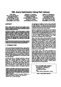
(a) Sample XML document
(b) Path synopsis
Figure 1: Sample XML document and corresponding path synopsis powerful as SJ or HTJ operators. Using them to the full extent, allows to significantly reduce: • CPU cost, because the time for deciding structural relationships by SJs or HTJs can now be saved • IO cost, as only a single access path has to be scanned.
1.2 Problem Statement To arrange the various SJ, HTJ, and access paths in such a way that the best possible plan is created, an optimizer’s plan enumerator applies various equivalence rules for generating alternative plans. In recent years, only SJ reordering has been considered in cost-based XML query optimization settings [25]. Even though this approach is self-evident because it proved to be effective in relational query optimization, it does not pay attention to the various HTJ operators and indexes proposed in the literature. Today, we cannot be sure that SJ reordering is still the most effective strategy for XML query optimization. Therefore, the optimizer must be able to take advantage of both of them. Although TAPs provide functionality comparable to materialized views in relational database systems and allow to quickly access all instances of a specific path in an XML document, recent optimization approaches do not consider them, too. As we have argued in Section 1.1, exploiting TAPs helps to reduce IO and CPU costs dramatically while making the overall QEP much simpler, because the number of operators is reduced significantly. Currently, other authors are only focusing on cost-based XPath optimization. As XQuery is becoming the de-facto query language for XML, FLWOR expressions and other fancy language features add additional complexity and further increase the search space for optimizers tremendously.
1.3 Our Contribution In summary, this paper contributes the following: • We describe the cost-based XQuery optimizer implemented in the XML Transaction Coordinator (XTC)— a full-fledged native XDBMS. • We provide a set of plan-equivalence rules that allow to take advantage of SJs, HTJs, PAPs, SAPs, and TAPs. • We introduce a cost model that is used by our optimizer. • We empirically evaluate the reliability of our cost model and assess the effectiveness of our optimization approach for XQuery/XPath queries.
1.4 Related Work In this section, we give a brief assessment of relevant publications on relational cost-based query optimization, optimization frameworks, and XML query optimization.
Cost-Based Query Optimization in RDBMSs. Selinger et al. [22] proposed the first cost-based query optimizer, which was part of System R—the prototype of the first relational database system. The optimizer was capable of optimizing simple and linear SPJ (select, project, and join) queries. The authors introduced a simple cost model based on weighted IO and CPU costs and used statistics on the number of data pages consumed by relations to bind the cost model’s variables to concrete values. Their dynamic programming algorithm initially selects optimal operator fittings for access paths. Thereafter, an optimal join order is determined based on a local optimality assumption. To early prune the search space, not all possible enumerations are taken into account. Instead, they only focus on interesting join orders, i. e., orders that do not require additional introductions of Cartesian products. Graefe and DeWitt [10] presented the EXODUS Optimizer Generator. This system is not tailored to a specific data model and supports the specification of algebraic transformations as rules. Together with a concrete data model, these rules serve as input for an optimizer generator, which creates a tailor-made query optimizer. The Starburst project [19] contributed important concepts to the emerging research field of query optimization. Among other things, the authors present the so-called Query Graph Model (QGM)—an extended relational algebra with a strong emphasis on structural relationships between language constructs. Beyond that, they introduced the concepts of rulebased query optimizers that can be easily modified by adding new rules for query transformation and query translation. Hence, this approach greatly improves the extensibility of such systems. The Volcano project [11] as well as the Cascades project [9] are heirs of the EXODUS project. The authors distinguish between transformation rules, which serve for algebra-toalgebra transformations, and implementation rules describing the mapping from logical algebra expressions to operator trees. In contrast to the System R approach [22], they use a top-down query optimization algorithm that first takes a bird’s eye view on QEPs.
Query Optimization Frameworks. Lanzelotte and Valduriez [14] contributed an extensible framework for query optimization that models the search space independent of a particular search strategy. Using this approach, developers can build highly-extensible plan enumeration frameworks. Kabra and DeWitt [13] proposed OPT++ as an objectoriented approach for extensible query optimization. By combining an extensible search component with an extensible logical and physical algebra representation, they lift the work of Lanzelotte and Valduriez to the object-oriented level.
XML Query Optimization. The classic work of McHugh and Widom [16] on the optimization of XML queries only targets at the isolated and strictly limited problem of optimizing path expressions using navigational access paths and lacks support for SJ and HTJ operators. Wu et al. [25] proposed five novel dynamic programming algorithms for structural join reordering. Their approach is orthogonal to our work, i. e., it can be employed to choose the best join order in SJ-only scenarios. Compared to our work, they use only a very simple cost model for driving the join-reordering process and do not consider the combination of SJ and HTJ operators as well as different index-based access operators. Zhang et al. [26] introduced several statistical learning techniques for XML cost modeling. In contrast to our work, which will follow a static cost modeling approach, they demonstrate how to describe the cost of a navigational access operator. Unfortunately, they do not cover set-oriented SJ and HTJ operators. Balmin et al. [3] sketch the development of a hybrid costbased optimizer for SQL and XQuery being part of DB2 XML. Compared to our approach, they evaluate every path expression using an HTJ operator and cannot decide on a fine-granular level whether to use SJ operators or not. Che et al. [5] describe an XPath optimization framework that performs so-called deterministic (algebraic) optimization. They provide no cost-based optimization framework and do not use a full-fledged DBMS as testbed. Georgiadis et al. [7] describe a first approach to cost-based XPath optimization. In contrast to our proposal, which supports the optimization of XQueries, too, they do not consider HTJs and advanced access paths like path indexes or CAS indexes.
2.
PRELIMINARIES
Our XQuery optimization framework is part of the XML Transaction Coordinator (XTC)1 , which is our prototype of a native XDBMS providing full transaction support and differing APIs for accessing XML data (e. g., DOM, Sax, and XQuery). To understand the cost formulae (Section 3.2) of the various access paths, we first describe their physical representation in our system. To enable efficient evaluation of structural predicates, a node labeling scheme is required, that assigns each node in an XML document a unique identifier that enables to decide for two given nodes the XPath axis they are related to—without further document access. As a prefix-based labeling scheme, DeweyIDs [18] qualify very well for this job. For example, Figure 1(a) shows an XML document that is 1
Project website: http://www.xtc-project.de
labeled with DeweyIDs. By just looking at the DeweyIDs, we can see that book (label 1.5.5 ) is a child node of books (label 1.5 ), because they share the same prefix and their level information (total number of odd figures separated by “.”) differs only by one. Figure 1(b) depicts the corresponding Path Synopsis (PS) for the document shown in Figure 1(a). A PS is a structural summary, which is actually an extended Data Guide [8], that is annotated with so-called Path Class References (PCRs). Every PCR refers to a unique path in the document. For example, PCR 3 refers to all /bib/books/book paths. Furthermore, the PS provides statistical information on the number of instances of each PCR. Figure 2(a) shows the document index. The document index is our PAP, i. e., our default access path, that simply indexes the complete document using the DeweyIDs as keys. Using a shared scan over it, inputs for SJ, HTJ, and navigational primitives can be provided. Figure 2(b) illustrates a SAP providing efficient access to specific element nodes. The element index is a two-stage index where element names (e. g., book) serve as keys in the name directory. Each entry points to a nodereference index that contains all nodes in document order having the same element name.
(a) Document index
(b) Element index
Figure 2: Primary and secondary access path Tertiary access paths provide advanced query processing capabilities. They can be considered as materialized views on paths in an XML document. Our system provides a path index and an additional content-and-structure (CAS) index, which both can have their values clustered by PCRs or DeweyIDs.
(a) Path index
(b) CAS index
Figure 3: Tertiary access paths Figure 3(a) shows a path index for our sample document. Here, the tuple (PCR, DeweyID) serves as key in the index. For example, if we want to evaluate the path expression/bib//book/title, we can use the knowledge on the document’s structure provided by the PS. Thus, we can infer that we will find all nodes satisfying the path expression by scanning the path index for all records having PCR 6. Content-and-structure (CAS) indexes support paths that end on content nodes (attribute or text content). Here, the content node’s value serves as key in the index. The indexed value is formed by a tuple (PCR, DeweyID) or (DeweyID, PCR), depending on the clustering. Figure 3(b)
illustrates a CAS index (with PCR clustering) that is defined for the content nodes of the path /bib/books/book/title and /bib/books/book/author, respectively. As we have already discussed in Section 1.1, CAS indexes are a potent means for supporting the efficient evaluation of point or range predicates on content nodes. They are extremely helpful, because, in contrast to structural relationships, which can be decided by just looking at the DeweyIDs of the involved nodes, the evaluation of value-based predicates would otherwise require more expensive accesses to a content index or—even worse—to the document index.
3.
OPTIMIZATION FRAMEWORK
The sequence-based XML Query Graph Model (XQGM), which is an extension to the seminal Query Graph Model (QGM) [19], serves as solid foundation for our query optimization approach. The XQGM is equivalent to the XQuery Core Language (normalized version of XQuery without syntactic sugar) and supports the most important concepts of XQuery 1.0 such as FLWOR expressions and node construction. After normalizing an XQuery expression, several algebraic rewrites (e. g., query unnesting) are applied to get rid of the node-at-a-time evaluation (especially all the nested forloops for the evaluation of structural relationships) inherent to the XQuery Core Language. Furthermore, text() accesses are pushed up as much as possible. After query rewrite, we get an XQGM representation where almost all operators follow the classical set-at-a-time processing paradigm, because, now, all structural relationships are evaluated using logical SJs. We can pass on this representation to the query optimizer that selects the best join order, optimal operator implementations, and the cheapest access paths. Due to the lack of space, we cannot give a full introduction to the XQGM. Instead, we only briefly sketch the XQGM representation for an XQuery expression2 . In Figure 9 (Appendix), you can see a slightly simplified version of XMark benchmark query Q11. Each XQGM operator receives and produces (nested) sequences of DeweyIDs enriched with PCRs and probable content nodes. In addition to the Select operator provided by the classical QGM for the evaluation of value-based joins, the XQGM provides a logical SJ operator that joins two sequences of node IDs based on their structural relationships, which can be decided using their corresponding DeweyIDs. The SJ operators receive their initial inputs from Access operators that provide access to the node labels of element or attribute nodes. The Group By operators group their inputs by doc("auction.xml")//person. The Merge operator filters out all doc("auction.xml")//person subtrees that do not have profile/@income and name subtrees, respectively. Furthermore, for each $p/name that satisfies the merge predicate, the text() expression is evaluated. The projection specification (PROJ_SPEC) describes which tuple sequences are passed on to the subsequent operator. Each operator is connected to a tuple variable (filled circles) that can have three different quantifiers: for (F), let (L), and exists (E). In this example, only F and L are used, which express the corresponding XQuery language constructs. For 2 A formal definition of the syntax and semantics of the XQGM is provided by Mathis [15].
F-quantified tuple variables, a full iteration over their input is performed, whereas L-quantified tuple variables just bind the complete input sequences for predicate evaluation. The top-most Select operator (below the output node) materializes the query result. The second Select operator evaluates a value-based join (as given in the where clause). Solid lines describe the direct data flow, whereas the dotted line refers to the provisioning of the current evaluation context. Here, the Select operator’s left tuple variable receives the current evaluation context. For each sequence item provided by the context, the value-based join predicate is evaluated for each tuple received via the right tuple variable that provides all tuples that satisfy the following expression: doc("auction.xml")//initial. This section is organized as follows: In Section 3.1, we describe the equivalence rules that enable the plan enumerator to generate alternative plans. Next, the cost model that allows the plan enumerator to prune expensive plans is presented in Section 3.2.
3.1 Plan Equivalences At the beginning of query optimization, for every XQGM instance, a corresponding plan (which normally consists of subplans) is derived. A plan encompasses all static properties of the corresponding XQGM instance, e. g., structural predicates, projection specifications, or orderings that have to be preserved. In addition to that, each plan contains dynamic properties, e. g., required sorting on inputs, cost estimates, and the currently assigned physical operator. In contrast to static properties, dynamic properties may change during every state transition. For a more convenient formulation of the plan equivalences, we use the following nomenclature: We denominate a plan and its properties by P[p1 , . . . , pn ], whereas P is the type of the plan and the properties p1 . . . pn are enclosed in squared brackets. For our equivalence rules, we distinguish between the following types of plans: Pi A plan of an arbitrary type Aj Access plan (scan over a PAP or SAP) SJt Structural Join of type t (omitted if irrelevant) HTJ Holistic Twig Join TAP Scan over a TAP Every plan may have several of the following properties: I Currently assigned physical operator P Predicate (e. g., XPath axis) D Input sequences where duplicates must be removed O Sequences to be projected out Consecutively, we use the following notation to describe the plan equivalences: P1 ≡c P2 . This reads: plan P1 is equivalent to plan P2 iff the condition c is satisfied. To not compromise readability, we only give informal definitions of c.
Implementation Exchange. Let Op be the set of all physical operators available to the optimizer. The implementation (p1 ∈ Op ) of plan P can be changed iff there is another implementation p2 ∈ Op that implements P, too: P[I : p1 ] ≡c P[I : p2 ] Structural Join Associativity. In contrast to the relational world, where a single join associativity rule is sufficient, the
a) Structural join associativity
≡c
SJ⋊ [P : b//c, O : c, D : c]
SJ⋊ [P : a//b, O : b, D : b] P1 [O : a] b) Structural join commutativity
P1 [O : a]
P3 [O : c]
P1 [O : a]
P2 [O : b] ≡c
SJ[P : en−1 θn−1 en ]
An [O : en ]
P3 [O : c]
← − SJ [P : b θ a]
≡c
P2 [O : b]
...
SJ1 [P : b//c, O : {b, c}] P2 [O : b]
P2 [O : b] SJ [P : a θ b]
c) Structural join fusion
SJ⋊ [P : a//b, O : c, D : c]
P1 [O : a]
HTJ[P : e1 θ1 e2 , . . . , en−1 θn−1 en ]
A1 [O : e1 ]
A2 [O : e2 ]
...
An [O : en ]
SJ[P : e1 θ1 e2 ] A1 [O : e1 ]
A2 [O : e2 ] ≡c
SJ[P : en−1 θn−1 en ]
HTJ[P : e1 θ1 e2 , . . . , en−1 θn−1 en ]
A1 [O : e1 ] HTJ[P : e1 θ1 e2 , . . . , en−2 θn−2 en−1 ]
A1 [O : e1 ]
A2 [O : e2 ]
d) TAP detection
...
A2 [O : e2 ]
...
An [O : en ]
An [O : en ]
An−1 [O : en−1 ]
SJ[P : en−1 θn−1 en ]
...
≡c
TAP[P : e1 θ1 e2 , . . . , en−1 θn−1 en ]
≡c
TAP[P : e1 θ1 e2 , . . . , en−1 θn−1 en ]
An [O : en ]
SJ[P : e1 θ1 e2 ] A1 [O : e1 ]
A2 [O : e2 ] SJ[P : en−1 θn−1 en ]
TAP[P : e1 θ1 e2 , . . . , en−2 θn−2 en−1 ]
An [O : en ]
Figure 4: Structure-modifying plan equivalences
Operator
d) CAS index scan
IO Cost ˆ ˜ h(i) + PCard(i) − 1 · PageFetchCost ˆ ˜ h(in ) + h(ir ) + PCard(ir ) − 1 · PageFetchCost ˆ ˜ h(i) + ⌈PathSeli (e) · PCard(i)⌉ − 1 · PageFetchCost ˆ ˜ h(i) + ⌈PathSeli (e) · Sel(p) · PCard(i)⌉ − 1 · PageFetchCost
e) StackTree
CostIO (left) + CostIO (right )
CostCPU (left) + CostCPU (right )+ TCard(left) · EvalCost(p)
f) NavTree
CostIO (left) + TCard(left) · CostIO (right)
CostCPU (left) + TCard(left)· CostCPU (right ) · EvalCost(p)
g) Extended TwigOpt
CostIO (left) + CostIO (right )
CostCPU (left) + CostCPU (right )+ TCard(left) · EvalCost(p)
a) Document index scan b) Element index scan c) Path index scan
CPU cost TCard(i) · EvalCost(p) TCard(ir ) · EvalCost(p) PathCard(e) · EvalCost(p) PathCard(e) · Sel(p) · EvalCost(p)
Table 1: Cost formulae XML world makes things more complicated (orders must be preserved, early duplicate elimination). Therefore, we provide a set of Structural Join Associativity rules for different combinations of axes and output nodes [23]. For your convenience, we repeat the join associativity rule for two SJ operators evaluating the // axis and having the output node c. For example, this rule could be applied to reorder the following XPath expression a//b//c. In Figure 4 a, the corresponding plan equivalence is sketched. Here, arbitrary plans P1 , P2 , and P3 provide the sorted input sequences a, b, and c, respectively. On the left-hand side, two right semijoins (⋊) are used to calculate the structural relationships. Because in both cases, the // axis is evaluated, potential duplicates (on b and c, respectively) are eliminated early. On the right-hand side, a full join between the sequences of plan P2 and plan P3 is performed. Next, the result is joined with sequence a.
Structural Join Commutativity. Figure 4 b, shows the Structural Join Commutativity rule. This rule allows to exchange the left and the right join partner of an SJ by just ← − replacing the XPath axis θ by its reverse axis θ . Please note, this is only possible if θ is not the attribute axis.
Structural Join Fusion. Let e := e1 θ1 e2 , . . . , en−1 θn−1 en be a path expression with θ1 , . . . , θn ∈ {/, //}. By applying Structural Join Fusion, which is illustrated in Figure 4 c, on a cascade of SJs that evaluates e, we can iteratively replace it by a single HTJ. It is worth noting that the query optimizer is not forced to make a binary decision between an exclusive evaluation of e using SJs or HTJs. Moreover, the query optimizer can decide on a fine-granular level, i. e., for every path step ei θi ei+1 , whether it is cheaper to integrate it into the previously formed HTJ or not. Hence, the creation of hybrid plans consisting of SJs and HTJs is possible, too. TAP Detection. Until now, the plan equivalences of Figure 4 a–c are only able to create alternative plans consisting of SJs, HTJs, PAPs, and SAPs. Using them, we can already span a fairly large search space providing plenty of opportunities for optimization. Anyhow, we can now play our hand by considering TAPs. Using the TAP Detection
rule, the plan enumerator can generate further alternative plans by replacing a cascade of SJ operators (as depicted in Figure 4 d) or a HTJ operator by a single scan over an appropriate CAS or path index. For a path expression e := e1 θ1 e2 , . . . , en−1 θn−1 en with θ1 , . . . , θn ∈ {/, //} and its corresponding PCR pe , the query optimizer uses the PS to find out which indexes qualify as alternative access paths.
3.2 Cost Model In this section, we introduce a subset of our cost model (Table 1 a–g) that is relevant for understanding our query optimization approach. The evaluation cost of an operator is described by its IO and CPU costs. We only consider the CPU costs, if alternative plans have equal IO costs. The IO cost is estimated using the total number of pages that must be loaded into a cold database buffer. The total number of items, which must be processed, serves as estimate for the CPU cost.
TCard(x) PCard(x) PathCard(e) Sel(p)
Cost for fetching a page from disk and loading it into the DB buffer Total # elements in x. Total # pages consumed by x Total # instances of path expression e Selectivity of value-based predicate p
PathSeli (e)
=
h(i) EvalCost(p) Costx∈{IO,CPU} (y)
Height of index i Evaluation cost of optional predicate p Cost x of child operator y
PageFetchCost
PathCard(e) TCard(i)
Table 2: Constant and functions Table 2 shows the constant and functions used for the description of the various cost formulae. We currently use the EXsum framework [1] for cardinality estimation. In general, our approach can work together with arbitrary estimation frameworks. In particular, we chose EXsum, because it can provide reliable estimates even for rarely used axes like parent or ancestor.
Primary and Secondary Access Paths. In Figure 2(a),
4. PLAN ENUMERATION ALGORITHM
we illustrated the physical representation of the document index. Table 1 a shows the corresponding cost formula. For retrieving all element nodes with same name from document index i, we have to perform a full index scan. Foremost, we have to access the first leaf page resulting in h(i) page fetches. Next, we need to scan all leaf pages consumed by the index (PCard(d))3 . Compared to a document index scan, where the complete index must be read to get all element nodes having a particular name, the element index (Figure 2(b)) allows for finegranular access to specific element nodes. In order to reach the first entry of a node-reference index ir , we have to find the corresponding pointer in the name directory h(in ) and find the first leaf page (h(ir )). Table 1 b shows the complete formula.
In the context of this work, we use a bottom-up optimization strategy that is similar to the plan generation approach of System R. Algorithm 1 sketches the plan generation algorithm. Plan generation starts at the leaf nodes of the query graph (Access Operators). For every Access Operator, the getSuccessors functions returns all possible access paths. Using the prune function, only the cheapest alternative is retained. Next, for every inner node (currentPlan ) of the query graph (e. g., SJ or HTJ) the getSuccessors function creates all valid permutations (interesting SJ orders) of the subtrees residing on the Goal stack. For every combination, all matching plan equivalences (Table 4) are applied to currentPlan . The result is a set of equivalent plans differing in their implementation or arrangement of operators. The prune function estimates the costs of every plan s ∈ Successors and returns only the cheapest one (s′ ) that is marked as goal state and pushed onto the Open stack for the next iteration. All other states s ∈ Successors − {s′ } are dismissed. Finally, the algorithm terminates when the root of the query graph is reached and Open is empty. In Section 5, you can convince yourself that our plan generation algorithm traverses even large search spaces (e. g., some XMark benchmark queries have up to tens of thousands alternatives) at moderate cost.
Tertiary Access Paths. Figure 3(a) shows a path index i with PCR clustering for three different paths (PCRs 3, 6, and 7). Let us assume path expression e selects all paths having PCR 6. Furthermore, we postulate that all records have the same length. Then we can estimate the fraction of leave pages we actually have to touch using the PathSeli (e) (Table 1 c). For a CAS index, which allows for the evaluation of point as well as range predicates, Table 1 d shows the corresponding formula. For path indexes as well as for CAS indexes that are DeweyID-clustered, PathSeli (e) = 1.0 always holds, because their entries are now clustered according to their order of appearance in the document rather than their containment w. r. t. a specific path class.
Evaluation of Structural Predicates. In the context of this work, the query optimizer can choose between two implementations for an SJ operator: StackTree [2] and NavTree. StackTree is a classical binary SJ operator. The NavTree is equivalent to a relational nested-loops join. The cost formulae for both operators are shown in Table 1 e and Table 1 f, respectively. Besides binary join operators, our optimization framework provides an implementation for plans gained using Structural Join Fusion (4 c). The Extended TwigOpt operator— which adds, amongst others, grouping, evaluation of positional predicates, and support for negative predicates to TwigOptimal [12]—can be employed to evaluate path expressions or even more complicated structures like twigs in a holistic manner. Even though Extended TwigOpt is an n-way join operator, the cost formulae shown in Table 1 g depicts the binary case that can be easily generalized. The alert reader has already recognized that the cost formulae for StackTree and Extended TwigOpt are identical. They differ in the value provided by the function EvalCost(p) that returns the evaluation cost for the structural predicate p. The authors showed in [24] how to define this function in such a way that whenever Extended TwigOpt outperforms StackTree, EvalCost(p) is lower or higher, respectively. Using this approach, the query optimizer can decide for every binary structural relationship, whether it is cheaper to perform Structural Join Fusion or not. 3
We always decrease the total number of pages fetches by one, because we assume that the first page has already been loaded into the buffer in the previous step.
Algorithm 1: Search algorithm
1 2 3 4 5 6 7 8 9 10 11 12 13 14 15
Input: A stack Open with an initial plan Output: The stack Goal containing the cheapest plan according to the cost model Goal ← ∅; while Open.size() > 0) do currentPlan ← Open.pop(); if ¬ isGoal(currentPlan ) then Successors ← ∅; Successors ← getSuccessors(currentPlan ); Successors ← prune(Successors ); foreach s ∈ Successors do Open.push(s); end else Goal ← Goal ∪ {currentPlan }; end end return Goal ;
5. EMPIRICAL EVALUATION Access path Document Index Scan Element Index Scan Path Index Scan CAS Index Scan
PageFetchCost [ms] 0.78 2.48 2.45 1.85
Table 3: Optimizer settings Our experiments were done on an Intel XEON quad core (3350) computer (2.66 GHz CPUs, 4 GB of main memory, 500 GB of external memory) running Linux with kernel version 2.6.14. Our native XDBMS server—implemented using Java version 1.6.0 07—was configured with a page size of
Access path
Query
f
Est. IO
cording to the cost model, which was formed by using the available access paths and plan equivalences.
Act. IO
Doc. index
Full scan Full scan
2.0 10.0
9, 225 46, 260
9, 133 46, 451
Element index
//text //listitem //bidder
2.0 10.0 10.0
329.84 828.32 748.96
320.20 894.80 721.80
Path index
Path p1 Path p2
10.0 10.0
115.15 303.80
125.80 293.40
CAS index
Full, income Point, income Range, income
10.0 10.0 10.0
303.40 47.68 199.89
307.60 44.60 219.60
Table 4: Est. IO vs. actual IO on access paths In our first experiment, we verify the correctness of our cost formulae (Table 1 a–d). Table 4 shows the experimental results for different access patterns on XMark documents with different scaling factors (f = 1.0 ≈ 100 MB). For the document index, we performed full scans over the complete index. For the element index, we scanned three nodereference indexes of varying sizes. Furthermore, we defined path indexes on p1 =/site/closed_auctions/closed_auction and p2 =/site/people/person. Besides a full scan on the content of all income attributes, we also performed a point query (income = 9, 876.0), and a range query (20, 000.0 ≤ income ≤ 80, 000.0). On average, we get an error of less than 4%. Though our cost model is fairly simple, these results are promising. C2
C3
X X
X X X
X X X X
X X X X X
Primary Secondary Tertiary
X
Access path
Plan equivalence
Impl. exchange SJ associativity SJ commutativity Join fusion TAP detection
X X X X
Table 5: Optimizer configurations If not otherwise stated, for the remaining experiments, we query an XMark document with f = 6.0 (approx. 600 MB). To generate different plans, we use our bottom-up plan enumerator and three different optimizer configurations (Table 5). All of them can apply all plan equivalences except for the TAP detection. Configuration C1 can only use the document index as access path. In configuration C2 and C3, the optimizer can choose between the document index and element indexes. TAP detection is only allowed for configuration C3, because, here, path indexes and CAS indexes may be used in addition to the document index or element index. All TAPs were created using XTC’s auto-indexing mechanism [21]. The results reflect the optimal plan ac-
C1 C2 C3
10^7 Query Execution Time [ms]
10^6 10^5 10^4 10^3 10^2
10^6 10^5 10^4 10^3 10^2
A1
A2
A3
A4
A5
A6
A7
Query
(a) Estimated IO
A8
A1
A2
A3
A4
A5
A6
A7
A8
Query
(b) Evaluation time
Figure 5: PathMark-A results; f = 6.0 The second experiment tests our cost model on the PathMark-A queries4 (simple XPath expressions). These queries are all XPath queries consisting of several steps, but do not contain accesses to text() nodes. Here, selecting the best access path is crucial. If you have a look at Figure 5, you can see that the estimated IO is a good indicator for the overall query execution time. Please note, even though the optimizer chose the best SJ order or used an appropriate HTJ operator, the estimated IO as well as the execution time is worse. Using C2 accelerates query evaluation up to 99% (compared to C1). For C3, the cost model recommended the use of path indexes for all queries. As the execution timings indicate (Figure 5(b)), this was a good decision, hence, the execution time could be significantly reduced further. Name B1 B2 B3 B4
C1
C1 C2 C3
10^7 Estimated IO [ms]
16 KB and a buffer size of 256 16-KB frames. The experimental results reflect the average values of five executions on a cold database buffer. Table 3 shows the assignments to the constant PageFetchCost for the different access paths. All concepts described before, are implemented in the costbased query optimizer of XTC. Because our optimization framework is rule-based, we can easily tailor it to our needs.
Definition
C
doc(’auction.xml’)//asia/item[location= ’Germany’] doc(’auction.xml’)//asia/item[location > ’C’ and location = ’c’ and keyword 40000] [age