tive brain tumor segmentation system that incorporates 2D interactive and 3D automatic tools with the ability to ad- just operator control. The provided methods ...
An Interactive Graph Cut Method for Brain Tumor Segmentation Neil Birkbeck† Dana Cobzas† Martin Jagersand† † ‡ University of Alberta Cross Cancer Institute
††
Albert Murtha‡ Tibor Kesztyues†† University of Applied Sciences Ulm
Abstract
tion process, yet give the doctors full control over the segmentation.
Tumor segmentation from MRI data is an important but time consuming task performed manually by medical experts. Automating this process is challenging due to the high diversity in appearance of tumor tissue among different patients and, in many cases, similarity between tumor and normal tissue. We propose a semi-automatic interactive brain tumor segmentation system that incorporates 2D interactive and 3D automatic tools with the ability to adjust operator control. The provided methods are based on an energy that incorporates region statistics computed on available MRI modalities and the usual regularization term. The energy is efficiently minimized on-line using graph cut. Experiments with radiation oncologists testing the semiautomatic tool vs. a manual tool show that the proposed system improves both segmentation time and repeatability.
Although there exist good interactive segmentation tools for natural images [6, 25, 20, 1] that have extensions to 3D medical images [3, 22, 6, 11, 27], published interaction paradigms (scribbling for sample foreground/background statistics in region-based techniques or clicking on edge points for minimal path in contour-based techniques) are ineffective in the difficult task of brain tumor segmentation. This is due to both the overlapping intensity statistics of the tumor and the brain tissue as well as the tumor/edema often lacking well-defined boundaries. In addition, current interactive segmentation tools do not additionally provide a way of continuously adjusting the manual/automatic level of control as desired by medical doctors.
1. Introduction Brain tumor segmentation is essential for treatment planning and follow-up assessment. While many automatic algorithms have been proposed in the literature [16, 14, 23, 18], these have not made it into clinical use. Thus in practice, radiation oncologists spend a substantial portion of their time performing the segmentation task manually using one of the available visualization and segmentation tools (e.g., [24]). This is mainly due to tumor segmentation being a very difficult task [21]; therefore, there will always be cases when the automatic methods fail or perform poorly. Another consideration is that medical doctors must always have final control over the segmentation. The time consuming task of manually labeling brain tumors (and associated edema) also leads to considerable variation between doctors (∼ 80% [19]). Furthermore, in most settings the task is performed on a 3D data set by labeling the tumor slice-by-slice in 2D, limiting the global perspective and potentially generating sub-optimal segmentations. This motivates the need for an interactive segmentation tool that incorporates favorable aspects of the automatic methods (such as inter-slice consistency) to speed up the interac-
We propose an interactive method for brain tumor segmentation that overcomes some of the above mentioned difficulties. The method consists of 2D interactive and 3D propagation tools that are based on a common energy functional that incorporates region statistics computed over several image modalities, user constraints, and the usual regularization term. Defining our tools through such an energy functional makes our method more principled and robust compared to interactive methods based on morphological operations or region growing [26]. Using region statistics from several image modalities and over several slices allows our 2D slice-based interaction to maintain a degree of 3D consistency. Different degrees of interactive control are obtained through iterated use of the 2D tools, which are used to provide constraints for the semi-automatic 3D propagation tool. Additionally, the 2D tools allow a finer degree of manual/automatic interaction by introducing an extra weighted term in the energy functional that controls how much the segmentation adheres to the operator input. In this way, doctors can perform a hierarchical segmentation by continuously increasing the weight of their manual input. Based on feedback from medical doctors, we believe that this is the right segmentation paradigm for difficult segmentation tasks (such as brain tumors). The functional is efficiently minimized using graph cut [8]; restriction of the segmentation problem to a region around the user interaction allows real-time update of the
segmentation for the 2D tools. Our method is similar to GrabCut [25] but allows interactively changing the selection using a lasso or paintbrush tool (instead of the usual scribblings [6, 25]). We first formalize the problem as an energy minimization (Section 2) and give the modifications of the energy to allow user interaction and propagation (Section 3). Next we give the graph cut solution (Section 4) and details on the implemented segmentation system (Section 2 and 5).
2. Energy formulation of the segmentation problem Formally, image segmentation for a given image I can be defined as finding a curve C that partitions the image domain Ω ⊂ ℜ2 into two disjoint regions Ωin (object) and Ωout (background). The formulation of the segmentation problem in 3D is the same except that the segmentation is represented by a surface. When no distinct edges are present in the image, optimal segmentation can be obtained using an active region model (extension of the Chan-Vese [9]) that partitions the image only based on the regions’ appearance: E(C) = Edata P (C) + αEreg (C) P Edata (C) = − x∈Ωin log pin (x) − x∈Ωout log pout (x) Ereg (C) = |C| (1) where pin and pout are statistical models for data in the two regions (in/out) and |C| denotes the curve length and acts as a regularization (smoothing) term. Parameter α controls the balance between the data and the regularization terms, with large values of α giving smoother segmentations. Region statistics The MRI brain data has different modalities (T1, T1C, T2, FLAIR). At least two of them are present in most cases. We register them (using a rigid transformation) and compute pin /pout (tumor/brain) statistics from this vector valued data. We provide the choice of three different statistics (multivariate Gaussian, independent histograms, and multi-dimensional histogram). We noticed that the multidimensional histogram provides the best results.
Mt ˆt M
ˆt M
Mt Ωtin
Ωtin Ωtout
Ωtout pin ← (Ωtin ∪ M t ) pout ← (Ωtout \M t ) t+1 Ωin = (Ωtin \M t ) ∪
ˆt M
pin ← (Ωtin \M t ) pout ← (Ωtout ∪ M t ) t+1 ˆt Ωout = (Ωtout \M t ) ∪ M
Figure 1. Illustration of 2D interactive segmentation (left) and 2D interactive subtraction (right). Ωtout represents the previously segmented regions in all slices.
interactive continuous (level set, weighted distance) techniques [11, 2] where the segmentation discriminates between two regions based on statistics that are learned from user scribblings (marking foreground/background pixels). In tumor segmentation, region statistics for tumor/brain tissue generally overlap and a few pixels of user scribbling are not enough to distinguish between them. We therefore designed an interactive segmentation technique that allows intuitive local control over the segmentation using 2D operations, where the user interaction influences the in/out statistics by drawing a region that contains the segmentation. After several 2D slices have been segmented we propagate the segmentation to the 3D volume.
3.1. 2D Interactive Tools The foundation for our 2D tools is that interactive updates should only be applied to a local region, e.g., a user supplied mask, M t , which can either be obtained from a paint-brush or a lasso-type tool. Given such a region, we incorporate the information of the user selected region into the currentSsegmentation, Ωtin by taking region statistics pin from Ωtin M t and pout from Ωtout \M t . The segmentation energy (Eq. 1) is solved using these updated region statistics and local control is obtained by updating the current segmentation only within the operator selection. Formally, ˆ t = argmin E(C) being the segmenwith Ω = M t and M tation restricted to M t , the segmentation is updated as follows:
3. Interactive segmentation & propagation
t t ˆt Ωt+1 in = (Ωin \M ) ∪ M
(2)
Two major paradigms for existing interactive segmentation tools are: (1) Contour-based methods like intelligent scissors [20] or live-wire [1] suitable for edge-based segmentation. The user indicates pixels where the segmentation boundary should pass and the segmentation is achieved as the shortest path according to an energy based on gradients. (2) Region-based interactive graph cut [6, 25] or
t+1 Ωt+1 out = Ωin
(3)
Refer to Figure 1 (left) for an example of the process. The region statistics are taken from all segmented slices, which allows the system to learn region statistics from the user selections throughout the volume. Furthermore, incorporating user input in this way requires no bootstrapping,
Figure 2. A typical user interaction with a square brush (green). Initially, pin and pout are extracted using the brush location. As the user sweeps the brush around the contour, the segmentation (red) and the region statistics are updated to include the newly segmented region. The user only provides a coarse path around the boundary (green trails) but the recovered segmentation accurately delineates the tumor (red).
Figure 3. A typical user interaction with a lasso. The user adds a selection to an existing segmentation (red). The segmentation is updated within the users selection in real-time as the selections the region to be modified.
meaning our approach allows Ω1in to be empty. Figure 2 illustrates an example stroke (e.g., over time, t) starting with no initial segmentation. Figure 4 illustrates a similar interaction over time with the lasso. Positive/Negative segmentation The interactive segmentation method described above is used to add regions to the current segmentation - “positive behaviour”. Similarly we defined a “negative behaviour” that subtracts regions from the current segmentation. Refer to Figure 1 (right) for an illustration. In this case, the new region statistics are calculated by subtracting M t from the inside and adding it to the outside (e.g., pin is sampled from Ωtin \M t and pout from Ωtout ∪ M t ). This negative behaviour is defined by switching the roles of Ωin and Ωout in Eqns 2 & 3. See Figure 4 (a) for an illustration of the positive and (b) for negative segmentation. Adherence to user selection While in most cases it is desirable to benefit as much as possible from the automatic behaviour of the segmentation method, there will always be difficult cases when the automatic method performs poorly (even when restricted to a user selected region). We design another level of interaction that controls how well the recovered segmentation adheres to the user selection; it is controlled by balancing the in/out
data terms with a factor h. The adherence parameter, h, can take values from 0.5 (balanced terms, i.e., the usual energy scaled by 12 ) to 1 (manual behavior where all points inside the selected region are constrained to belong to the inside of the object). The energy restricted to a user supplied region, Ω = M t , is then: X X E(C) = − h log pin (x)− (1−h) log pout (x)+α|C| x∈Ωin
x∈Ωout
(4) See Figure 4 (b) for an illustration of a segmentation with increased adherence (notice that the red segmentation curve is closer to the green user selection compared to Figure 4 (a)).1 Adherence can be thought of as a prior; the segmentation prefers to adhere to the user provided region when h close to unity. Such a prior is similar to other priors in the literature (e.g., [13, 17]), where a segmentation that is closer to the prior shape is given a lower cost. Priors in this form have been used in similar difficult segmentation tasks (e.g., undefined boundaries, overlapping region-statistics between foreground/background) because graph-cut seeded/scribble approaches require too much manual interaction [13].
1 See
web page for video illustrating the adherence parameter [5]
(a) normal behavior
(b) increased adherence
(c) negative segmentation
Figure 4. Balancing automatic and manual control. Green lines show user selection and red lines shows updated segmentation.
3.2. 3D Propagation To obtain a degree of 3D interaction that leverages the consistency between slices, we adopt an approach similar to the 3D extensions of the 2D contour-based tools [12, 15]. Specifically, the operator performs segmentations on any 2D slice until satisfied and specifies that the segmentation should be fixed/locked on such a slice. In general, this type of interaction is easily integrated into the energy formulation, where we use a set of labels L : Ω → {−τ, 0, τ } (similar to [10]), with τ being some large number. The labels take on values of −τ for pixels fixed to be inside (tumor), τ for values fixed to be outside outside, and zero otherwise (i.e., the slice is not locked). The extra term to the energy functional in Eq. 1 is then X X Econs (C) = L(x) − L(x) (5) x∈Ωin
x∈Ωout
In this form, the labels enforce constraints on userconfirmed slices that have already been marked as ’in’/’out’, and ensure these values do not change during subsequent semi-automatic segmentation operations.
3.3. Comparison to existing methods Our 2D interactive technique allows the user to update the region statistics while maintaining accurate control over the region affected by the segmentation. Iterative updating of the region statistics is similar to methods like GrabCut [25]. But unlike our method, slight user interaction may have non-local effects in techniques like GrabCut; non-local behaviour is undesirable because a distant region where the segmentation had already been manually specified could be adversely affected. Restricting the region of interaction also allows for efficient real-time behaviour of our tool (also pointed out by [17]). Our adherence parameter, h, is similar to enforcing the user selection as a prior, which has been noted in the literature [17], but it has not been used
source ("tumor") 0 −log pin label q wpq p −log pout
e ∆φ
sink ("brain")
(a) graph structure
(b) edge neighborhood
Figure 5. 2D Graph structure and edge neighborhood.
in the context of continuous updating (adding/subtracting) to a segmentation as we do. Our description of 3D propagation of a segmentation is similar to the original interactive 3D methods where foreground/background scribbles are used for both region statistics and as hard constraints[6]. In our tool these constraints come from entire slices being locked. As such, they are also similar to the successful application of the 3D extensions of the contour-based approaches where 2D segmentations were propagated to other slices [12, 15]. Unlike these methods that solve the problem independently on each 2D slice, our propagation is performed in 3D while enforcing the 3D segmentation to obey these constraints.
4. Graph cut solution Several works (e.g., [7]) show that the type of energy presented in Eq. 4 with precomputed region statistics (pin , pout ) can be efficiently minimized using graph cut. Besides providing a global minimum to the segmentation energy, a graph cut solution is also fast and therefore suitable for the interactive techniques. Each pixel(voxel), p, in Ω is a node in the graph, and there are two special nodes: a source and a sink. Edge weights between a voxel-node and the
source/sink represent the data cost for the voxel: wp,src = −h log pin (p) and wp,sink = −(1 − h) log pout (p). Edges between neighboring voxels, p and q, encode the regularization cost. As shown by Boykov and Kolmogorov [7], the curve length is approximated on a graph system using ∆Φ the edge weights wpq = 2|epqpq| between neighbors p and q, where ∆Φpq represents the angle between two adjacent edge elements and epq is the vector associated with an edge. We use 16 neighbors for 2D segmentation and an 18 neighbors for 3D. Figure 4 illustrates the way the 2D energy is discretized on the graph. Created in this way, a cut in the graph isolates the source from the sink; points connected to the sink are labeled as “tumor” and points connected to the source as “brain”. It was shown [7] that the cost of a cut is equivalent to the segmentation energy from Eq. 4 and therefore the minimum cut gives global minimum of this energy. We used the maxflow algorithm from [8] in our implementation. The constraints used in the 3D propagation in Section 3.2 (Eq. 5) are implemented as hard constraints discretized directly on the graph by replacing the values corresponding to data edges with wp,src = 0, wp,sink = ∞ where L(p) = −τ and wp,src = ∞, wp,sink = 0 where L(p) = τ . The local graph cut in region M t (new user selection) with recomputed region statistics based on the same user selection (as explained Section 3 and Figure 1) is solved ˆ t is added to (positive behavior) or on-line. The solution M subtracted from (negative behavior) the previous segmentation as in Eq. 2 & 3. For 2D interaction, due to the efficiency of the graph cut solution when restricted to M t , the user sees the segmentation update on-line following his/her selection.
5. System/Implementation We integrated the interactive segmentation method into a system that provides a data visualization and an interactive interface. MRI data can have different modalities (T1, T1C, T2, FLAIR) that are visualized and manipulated in 2D (3 orthogonal views) as well as in 3D using volumetric rendering. The segmentation is visualized in both 2D as contours and in 3D as a surface, but the interactions with the segmentation take place in 2D slices in a manner familiar to doctors.2. 2D interactive tools The 2D interactive segmentation method presented in Section 3 is implemented using 2 types of tools - a lasso tool where the user selection is a mouse-driven curve and a paintbrush tool that selects brush strokes. Both tools have 2 The overview video gives an impression of how the tool can be used to perform a complete segmentation [4]
adjustable levels of smoothness (regularization parameter α) and adherence (parameter h in Eq. 4), and both tools can add or subtract regions. The segmentation is as fast and responsive as using a manual tool. Recomputing the segmentation within a 19x19 square brush along a stroke, including recomputing region statistics, takes roughly 0.01-0.02s on a 2.4GHz machine for each cursor position. Roughly half of the time is spent recomputing region statistics as it considers the segmentation in the entire volume; this could be improved by caching statistics from other slices. 3D propagation After a few 2D slices have been segmented, sufficient data for region statistics is available, and the result can be propagated to 3D. Any 2D slices the operator has segmented may be enforced as a hard label by “locking” the segmentation on the slice. The 3D propagation is obtained minimizing the same energy (Eq. 1) in 3D while maintaining the hard label constraints provided on individual slices. The 3D segmentation is done incrementally; each time the tool is involved the segmentation volume is constrained to lie within a certain distance of the current segmentation volume. Region statistics are calculated from the sample slices and updated at each step. The operator is free to interact and lock more slices during the incremental application of the 3D segmentation. Figure 6 shows an initial segmentation and the result of the 3D propagation. Invoking the 3D propagation for a volume of 256x256x33 with 6 locked slices, where the selection is an average of 100x100 on the locked slice (e.g., a total of 270385 nodes in the graph) takes roughly 2 seconds. The propagation of a similar setup on a 512x512x33 resolution volume (814049 graph nodes) takes about 8 seconds.
6. Experiments and Discussion To evaluate the semi-automatic system we asked two expert radiation oncologists and two novices to use it on two data sets, each containing 20 MRI slices in two modalities (T1C and FLAIR). The 4 users were asked to segment each dataset twice, once in manual mode and once in semiautomatic mode (in what order they prefer and not one after the other to avoid the learning effect). One expert and one novice segmented each dataset 6 times (3 manual, 3 automatic). In manual mode the operator manually delineated the tumor with a standard paint-brush and lasso tool. We measured the time needed to perform each segmentation and the intra/inter-user repeatability. Intra- and interuser repeatability scores average the overlap (Jaccard score) between pairs of same segmentations (same dataset and same manual or automatic mode) done by the same person (the expert that segmented each data 6 times) for intra-user
initial slice
initial 3D
example final slices
final 3D
Figure 6. Example of 3D propagation.
expert novice
time (min) manual auto 7.25 1.97 11.93 4.5
intra-user repeat. (% overlap) manual auto 83.72 93.67 78.71 90.53
inter-user repeat. (% overlap) manual auto 67.65 76.76 70.84 79.57
Table 1. Results for manual/automatic experiments. The time is measured in minutes and the repeatability is measured using the Jaccard (overlap) score: Jaccard(A, B) = (A ∩ B)/(A ∪ B)
repeatability or different persons (expert-expert or noviceexpert) for inter-user repeatability. The results presented in Table 1 show that the segmentation done using the semi-automatic tools is about two to three times faster than with manual labeling while the inter/intra-user repeatability is about 10% smaller. The manual inter-user repeatability was about 80% (matching the result from [19]) and improved to 90% consistency using our tool. This important consistency improvement is due to the fact that the same region statistics on all available modalities are propagated and used globally, instead of the doctors using a local 2D perceptual measure on one slice and modality at a time.
7. Conclusion We presented an interactive method for brain tumor segmentation. The method is incorporated into a segmentation system that provides 2D interactive and 3D propagation tools based on graph-cut techniques. Novel improvements incorporated are continuous balance adjustment of operator control with an adherence parameter and the on-line 2D user interaction through a lasso and a brush tool (and not the point clicking and scribblings used in previous interactive segmentation). This results in better control over the segmentation by significantly changing the region statistics and by bounding the segmentation. Experiments prove that the proposed tool speeds up the segmentation and reduces intra- and inter-user repeatability when compared with conventional manual segmentation. Future improvements for our interactive techniques include extending the 2D brush tools to 3D and adding the ability to lock orthogonal slices for the propagation (e.g.,
like the live-wire extensions [12, 15]). Other improvements include investigating whether optimal parameter selection can be performed for the smoothness/adherence parameters (similar to [1]), e.g., by instructing the operator to first make a manual segmentation, fitting a coarse stroke to this region, and finding the parameters that bring the graph cut segmentation into close alignment.
References [1] a. Alexandre X. Falc J. K. Udupa, S. Samarasekera, S. Sharma, B. E. Hirsch, and R. de A. Lotufo. Usersteered image segmentation paradigms: live wire and live lane. Graph. Models Image Process., 60(4):233–260, 1998. [2] G. S. Alexis Protiere. Interactive image segmentation via adaptive weighted distances. IEEE Transactions on Image Processing, 16(4):1046–1057, 2007. [3] C. J. Armstrong, B. L. Price, and W. A. Barrett. Interactive segmentation of image volumes with live surface. Comput. Graph., 31(2):212–229, 2007. [4] N. Birkbeck, D. Cobzas, M. Jagersand, A. Murtha, and T. Kesztyues. Video of a complete user segmentation. http://www.cs.ualberta.ca/˜vis/sass/p/wacv09/overview.wmv. [5] N. Birkbeck, D. Cobzas, M. Jagersand, A. Murtha, and T. Kesztyues. Video overview of adherence parameter. http://www.cs.ualberta.ca/˜vis/sass/p/wacv09/adhere.wmv. [6] Y. Boykov and M.-P. Jolly. Interactive graph cuts for optimal boundary and region segmentation of objects in n-d images. In ICCV, pages 105–112, 2001. [7] Y. Boykov and V. Kolmogorov. Computing geodesics and minimal surfaces via graph cuts. In ICCV, pages 26–33, 2003. [8] Y. Boykov and V. Kolmogorov. An experimental comparison of min-cut/max-flow algorithms for energy minimization in computer vision. IEEE PAMI, 26(9):1124–1137, 2004.
[9] T. Chan and L. Vese. Active contours without edges. IEEE Trans. Image Processing, 10(2):266–277, 2001. [10] D. Cremers, O. Fluck, M. Rousson, and S. Aharon. A probabilistic level set formulation for interactive organ segmentation. In Proc. of the SPIE Medical Imaging, San Diego, USA, February 2007. [11] M. Droske, B. Meyer, M. Rumpf, and C. Schaller. An adaptive level set method for medical image segmentation. In IPMI: Proceedings of the 17th International Conference on Information Processing in Medical Imaging, pages 416–422, 2001. [12] A. X. Falco and J. K. Udupa. A 3d generalization of usersteered live-wire segmentation. Medical Image Analysis, 4(4):389 – 402, 2000. [13] D. Freedman and T. Zhang. Interactive graph cut based segmentation with shape priors. In CVPR ’05: Proceedings of the 2005 IEEE Computer Society Conference on Computer Vision and Pattern Recognition (CVPR’05) - Volume 1, pages 755–762, Washington, DC, USA, 2005. IEEE Computer Society. [14] D. Gering. Recognizing Deviations from Normalcy for Brain Tumor Segmentation. PhD thesis, MIT, 2003. [15] G. Hamarneh, J. Yang, C. McIntosh, and M. Langille. 3d live-wire-based semi-automatic segmentation of medical images. In SPIE Medical Imaging, pages 1597–1603, 2005. [16] M. Kaus, S. Warfield, A. Nabavi, P. Black, F. Jolesz, and R. Kikinis. Automated segmentation of MR images of brain tumors. Radiology, 218:586–591, 2001. [17] C. Liu, F. Li, and S. Zhan. Interactive dynamic graph cut based image segmentation with shape priors. MIPPR 2007: Automatic Target Recognition and Image Analysis; and Multispectral Image Acquisition, 6786(1):67862I, 2007. [18] J. Liu, J. Udupa, D. Odhner, D. Hackney, and G. Moonis. A system for brain tumor volume estimation via mr imaging and fuzzy connectedness. Comput. Medical Imaging Graph., 21(9):21–34, 2005. [19] G. Mazzara, R. Velthuizen, J. Pearlman, H. Greenberg, and H. Wagner. Brain tumor target volume determination for radiation treatment planning through automated mri segmentation. Int. J. of Radiation Oncology Biology Physics, 59(1):300–312, 2004. [20] E. N. Mortensen and W. A. Barrett. Intelligent scissors for image composition. In SIGGRAPH, pages 191–198, 1995. [21] M. R. Patel and V. Tse. Diagnosis and staging of brain tumors. Semonars in Roentgenology, 39(3):347–360, 2004. [22] K. Poon, G. Hamarneh, and R. Abugharbieh. Segmentation of complex objects with non-spherical topologies from volumetric medical images using 3d livewire. In SPIE Medical Imaging, pages 1–10, 2007. [23] M. Prastawa, E. Bullitt, S. Ho, and G. Gerig. A brain tumor segmentation framework based on outlier detection. Medical Image Analysis, 8(3):275–283, 2004. [24] R. Robb, D. Hanson, R. Karwoski, A. Larson, E. Workman, and M. Stacy. Analyze: a comprehensive, operatorinteractive software package for multi-dimensional medical image display and analysis. Computerized Medical Imaging and Graphics, 13(6):433–454, 1989.
[25] C. Rother, V. Kolmogorov, and A. Blake. ”grabcut”: interactive foreground extraction using iterated graph cuts. ACM Trans. Graph., 23(3):309–314, 2004. [26] W. A. K. Yan Kang, Klaus Engelke. Interactive 3d editing tools for image segmentation. Med Image Anal., 8(1):35–46, 2004. [27] P. A. Yushkevich, J. Piven, H. C. Hazlett, R. G. Smith, S. Ho, J. C. Gee, and G. Gerig. User-guided 3d active contour segmentation of anatomical structures: Significantly improved efficiency and reliability. NeuroImage, 31(3):1116 – 1128, 2006.