An Interactive Learning Module in Preparation for Integral Methods in Fluid Mechanics Loren Sumner1
Abstract – A lecture for a fluid mechanics course in mechanical engineering has been developed to provide experiences for students that aid in their abilities to envision basic fluid mechanics concepts. Lecturing in a computer laboratory, students interact with CFD post processing software to dynamically visualize the flow field of a simple curved-pipe-flow problem while observing a lecture explaining opportune topics and directing efforts to complete a worksheet. This departure from a traditional lecture style is referred to as a learning module and occurs once in the semester at a point appropriate to introduce integral analysis methods. A description of the learning module and formative assessment results are discussed. Keywords: Experiential Learning, Active Learning, Fluid Mechanics, Computer Aided Engineering, Computational Fluid Dynamics
INTRODUCTION A teaching-enhancement project at the Mercer University School of Engineering (MUSE) focuses on incorporating sparse usage of computer-aided-engineering (CAE) resources to teach engineering fundamentals. The general benefits of CAE in engineering practice are well evident via visualizations with powerful 3-D graphics rendering solid models and intricate results from numerical simulations. Just as these resources increase engineering potential for companies and attract customers, CAE should have the potential to impact teaching and learning in engineering education and attract students. The project established the Keck Engineering Analysis Center at MUSE housing a cluster of SUN workstations with state-of-the-art engineering software. The Center seeks to expose students to CAE tools typical in industry, extend the analysis capabilities of student scholarship such as senior design, and most importantly, to enhance the pedagogy of select engineering topics. Rogge, Burtner and Sumner [1] present a comprehensive description of the project. With careful focus on enhancing pedagogy of engineering fundamentals, learning modules are being developed to consist of a lecture, or two, in a computer laboratory utilizing prearranged dynamic visualizations and limited student-computer interaction. Learning modules intend to enhance lectures of targeted pre-existing course topics and do not warrant laboratory credit hours. Four disciplines participate in the project; Biomedical, Computer, Industrial and Mechanical engineering. Examples of these learning modules, other than the module presented herein, can be found in various conference proceedings [2-4] discussing learning objectives, implementation strategies, and assessment. Fluid mechanics represents one of many Mechanical engineering courses implementing learning modules at MUSE. Currently, a single learning module in fluid mechanics reinforces and introduces several basic fluid-flow concepts. While discussing basic concepts, the module contributes to the students’ practical experience in fluid mechanics and CAE.
1
Department of Mechanical Engineering, Mercer University, 1400 Coleman Ave., Macon, GA 31207;
[email protected] 2005 ASEE Southeast Section Conference 1
Studies of teaching and learning recognize the importance of experiences[5, 6]. Experience promotes common sense and intuition, and can logically play a significant role in the learning process. For example, Kolb’s educational model[6] suggests four stages of learning: active experiences, reflective observations, abstract conceptualization, and active experimentation. The model intends for a nominal progression through the stages sequentially. Thus, experience is important early in the learning process rather than later. Regarding the traditional education format, beginning a course with a lecture must presume some level of prior experience among the students, and working homework problems serves as the obvious means for active experience. As most engineering courses, fluid mechanics involves applying basic principles with consequential calculations. In fluids however, these applications must serve a wide assortment of situational flow characteristics. These characteristics are categorized as laminar or turbulent flow, internal or external flow, ideal or viscous flow, etc. Overall, fluid mechanics can appear to those with little experience as many disjoint topics thrown together due to a single commonality: the consideration of a fluid. It is logical then to consider the categories and possible complexities of fluid mechanics in the introductory material of a course to provide structure or framework for organization of later subjects. Many fluid mechanics textbooks such as Fox et al.[7] implement such a theory. On the other hand, all of this framework material could contribute to a general confusion initiated with the beginning topics. The fluid mechanics learning model described below aims to provide active experience at a point in the semester when some basic concepts and general flow categories can be reinforced while preparing students for new topics employing integral methods.
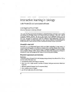
MODULE DESIGN The introductory material of a fluid mechanics course in mechanical engineering includes some immediately pertinent concepts such as viscosity, shear stress, and the definition of a Newtonian fluid, plane viscometers, etc., but also addresses, to varying degrees, an assortment of topics which are preparatory and intended to provide a framework for the remaining studies in the course. Preparatory type discussions would consider the nature of laminar and turbulent flow, boundary layers and wakes, internal and external flows, etc. Beyond the introductory material, topics for the remainder of the course address, in a similar order, fluid statics, elementary dynamics, control volume analysis, local analysis, dimensional analysis, internal flows, etc. The learning module uses computational-fluid-dynamics (CFD) results to discuss the laminar pipe flow problem shown in Figure 1. The problem considers a uniform entrance velocity profile, a 45-degree bend, and then discharges to atmospheric pressure. A specified mass flow rate of 0.01402 kg/s provides a Reynolds number of approximately 2000 ensuring laminar flow of water at 25oC.
Water (25 oC)
Discharge to Atmosphere 10cm
R = 2 cm 45°
10cm 1cm
Figure 1 – Problem specifications. 2005 ASEE Southeast Section Conference 2
Ideally, the module constitutes a single lecture about five weeks into a 15-week semester to follow lectures addressing elementary dynamics and precede lectures on control volume analysis. Students are guided through step-by-step, point-and-click procedures to interactively observe images from prepared post-processing results. Students are free to investigate by repositioning and rotating images as desired. An in-class worksheet accompanies the lecture with relevant calculations to be completed as directed by the instructor. The module intends to: 1) demonstrate flow visualization concepts including streamlines, pathlines, vector field and contour plots, 2) reinforce basic topics such as viscosity, shear stress, velocity profiles, volumetric flow rates, 3) bare witness and discuss advanced topics such as boundary layers and developing flow, the no slip boundary condition, pressure-driven pipe flow, and 4) review some relevant mathematical concepts in preparation for integral analysis topics such as setting up and evaluating surface integrals. Students should have experience in statics and dynamics to appreciate the concepts of a reaction force and momentum balance, and skills in basic calculus at a level sufficient to evaluate simple derivatives and surface integrals. Although not attempted with the current module design, the flow visualizations presented below provide an opportunity to also discuss topics of fluid kinematics such as the material derivative and convective acceleration. A complexity in the study of fluid mechanics stems from the need for such mathematical concepts to keep track of the motion of fluid particles in space and time and quantify the consequences from an Eulerian perspective. Additionally, some understanding of local fluid motion is essential even in solving problems with control volume methods. Visualizations The problem is solved with CFX-5, a commercial CFD software package. Postprocessing files are created to simplify viewing procedures required of students. Step-by-step visualization procedures are provided as a handout to students. Thus, students need not be familiar with the software, and the module makes no attempt to train students’ abilities with the software. The visualization procedures guide students through: 1) 2) 3) 4) 5)
a 2-D vector plot and speed contours of the center-plane velocity field, 3-D pathline animations (streamlines), 3-D surface plots of velocity over a pipe cross-section, 2-D pressure contours of the center-plane pressure field, and a shear-stress contour plot rendered on the pipe wall.
Figures 2a-b show samples of the resulting 3-D images. Speed contours of Figure 2a show the no-slip boundary condition and developing flow near the pipe entrance and around the 45-degree bend. Pressure contours of Figure 2b reveal the pressure gradient driving the flow as well as the transverse pressure change at the bend due to centripetal acceleration. The surface plot of Figure 2d intends to help students mentally visualize the velocity field and setup a surface integral specifying the volumetric flow rate. With the aid of these and other visualizations, formidable topics to be discussed at the instructor’s discretion include: 1) 2) 3) 4) 5) 6)
streamlines, timelines, pathlines, and streaklines, the no-slip boundary condition, developing versus fully developed flow, pressure-driven pipe flow, laminar versus turbulent flow, viscosity, shear stress and drag,
2005 ASEE Southeast Section Conference 3
7) boundary layers and internal versus external flows, 8) non-uniform velocity profiles and volumetric flow rates, and finally, 9) a balance of momentum. Worksheet The worksheet guides students through several concepts with calculations providing a more intense experience to complement the visualization. Students are not expected to be able to develop and complete many of the calculations independently due to the preparatory nature of some of the topics. Rather, students are guided through
a)
Center-plane speed contours
c)
3-D Pathlines
b)
Center-plane pressure contours
d) Surface rendering of velocity profile
Figure 2 – Sample visualizations of pipe flow solution
2005 ASEE Southeast Section Conference 4
calculations as a tutorial. The worksheet questions, presented in the appendix, address the following topics: 1) 2) 3) 4) 5)
finding fluid property values, velocity profiles in connection with flow rates, the critical Reynolds number for pipe flow, viscosity and shear stress, and applying the integral form of balance of momentum.
Ultimately via the worksheet, students will determine the minimum horizontal force required to hold the pipe in contact with the reservoir due to the interaction between the flowing water and the pipe. This resulting force is determined based on the CFD results and again analytically considering a fully developed laminar velocity profile. These calculations serve to prepare students to setup and solve surface integrals that will be necessary in the study of integral (control volume) analysis.
RESULTS AND ASSESSMENT The total of 21 students taking the course were able to amply follow the visualization procedures and seemed to enjoy the ability to explore the results by repositioning the pipe image. However, the expectation for all students to complete the worksheet in a timely manner proved to be unrealistic. Many students were unable to complete some of the worksheet questions without excessive attention from the instructor. The module as implemented consumed two 50-minute periods of lecture and still left the students to finish parts of the worksheet as homework. All students successfully completed the worksheet as homework. In comparison to the likely accomplishments of two traditional 50-minute class lectures, the module is arguably not a worthwhile venture. However, altering the implementation of the module by omitting the worksheet as an in-class activity would drastically decrease the time expense. The visualizations with sufficient discussion consumed approximately 30 minutes, and the worksheet could be assigned as homework. Alternatively, the worksheet could be utilized in a cooperative-learning lecture format where students would work in small groups to complete the worksheet. An extension to cooperative learning seems promising considering the benefits noted in previous studies and the already present teaching challenges of active learning [8, 9]. With the intent of experiential learning, specific objectives for the learning module, sighting student abilities to demonstrate calculations, were not identified. Instead, students were given a survey allowing them to convey their opinions of the experience. Figures 3-6 show the survey results of three questions. The information in the figures denotes the exact wording on the survey. Students were asked if the module helped them to understand course subjects. The distribution shown in Figure 3 has an average response of 3.15 on a scale of 1-5 as indicated. Additionally, no student was willing to claim that the module was essential to their learning, and no student claimed that the module was not at all helpful. Although the results indicate that 9 of 21 students benefited significantly from the module by indicating a response of 4, the overall impact on the class remains neutral. To query the students regarding their opinions of teaching effectiveness, they were asked if more or less time should be spent in the laboratory during lecture hours. Figure 4 shows the resulting distribution having an average of 3.05 on the indicated 1-5 scale. Again, a neutral impact shows a nearly symmetric distribution. Finally, students were asked to quantify the amount of time wasted due to technical (computer) issues. The average response indicates that 29.5 % of lecture time was wasted with two responses as high as 70 % and two as low as zero. Although a loss of nearly one third of the class time is inefficient, this incident marks the first implementation of this module and the students appeared uncomfortable working on UNIX based computers. Additionally students were asked, “Did the module improve your understanding of one or more particular fluids concepts that was otherwise unclear to you?” The results included 11 “yes” responses and 9 “no” responses. Following this question, space for comments was provided on the survey. Among the written comments, many students suggested that all relevant material be discussed in lecture before attempting the module calculations. 2005 ASEE Southeast Section Conference 5
10
9
9
Number of Students
8 7
6
6
5
5 4 3 2 1
0
0
0 1 - not at all helpful
2
3
4
5 - essential to my learning
Figure 3 – Students responses to “Did the class time spent in the Keck Engineering Analysis Center help you understand course subjects?” 9
8
8 Number of Students
7 7 6 5 4 3 3 2 1
1
1 0 1 - much more time needed
2
3 - just enough time
4
5 - much less time sufficient
Figure 4 – Students responses to “Considering the teaching effectiveness of the overall course, should more or less time be spent in the Keck Engineering Analysis Center?” 6 5
5
Number of Students
5 4 3 3 2
2
2 1
1
1
1 0
0
0
90
100
0 0
10
20
30
40
50
60
70
80
Percent of Time
Figure 5 – Student responses to “Of the class time spent in the Keck Engineering Analysis Center, how much was lost to non-engineering topics, such as learning software-specific procedures and/or issues regarding files or account problems?
2005 ASEE Southeast Section Conference 6
Recognizing that active experience is the first of four stages in Kolb’s educational model, the learning module attempted to support the future lectures of theory and concepts. Students’ preferences for more lecturing in preparation for the module suggest a sensitive balance between the first stage of active experience and the third stage of abstract conceptualization. In this case, the worksheet appears inappropriately challenging to be implemented immediately following the introductory lecture for integral methods. The survey results do not provide information for comparing the teaching effectiveness of the learning module to that of a traditional lecture. The results do show a potential for efficient teaching enhancements with continued development noting that nearly 50% of the students appear to have benefited from the learning module and that a great potential for improvement exists though the use of cooperative learning techniques and timing adjustments relative to lecture discussions. The learning module does succeed at providing a new experience for students not possible in a traditional classroom. The consequences of using UNIX based SUN workstations rather than PC’s are being assessed in conjunction with other learning modules of the Keck Center project.
ACKNOWLEDGEMENTS The efforts presented constitute a small component of a three-year multi-disciplinary project supported financially in its entirety by the W. M. Keck Foundation. Assistance in the development of a model problem from Dr. Sinjae Hyun of the Biomedical engineering department at MUSE is greatly appreciated.
REFERENCES [1]
Rogge, Burtner, Sumner, “Formative Assessment of a Computer-Aided Analysis Center: Plan Development and Preliminary Results,” Proceedings of the 2004 ASEE/IEEE Frontiers in Education Annual Conference, Savannah, GA., October 20-23, 2004.
[2]
Jenkins, H., “Increasing student interest and understanding in a first mechanics course through software modules,” Proceedings of the 2004 International Mechanical Engineering Congress and RD&D Expo, Anaheim, CA, November, 13-19, 2004.
[3]
Mahaney, J., “A drafting course for practicing engineers,” Proceedings of the 2004 International Mechanical Engineering Congress and RD&D Expo, Anaheim, CA, November, 13-19, 2004.
[4]
Ekong, D., “Using OPNET modules in a computer networks class at Mercer University,” Proceedings of the 2004 ASEE Southeastern Section Conference, Auburn, AL, April 4-6, 2004.
[5]
Keeton, M. T., Experiential Learning, Jossey-Bass Publishers, 1976.
[6]
Kolb, Experiential Learning: Experience as the Source of Learning and Development, Prentice-Hall, New Jersey, 1984.
[7]
Fox, McDonald, and Pritchard, Introduction to Fluid Mechanics, John Wiley & Sons, 2004.
[8]
Felder, R., Felder G., and Dietz, E., “A Longitudinal Study of Engineering Student Performance and Retention. V. Comparisons with Traditionally-Taught Students,” Journal of Engineering Education, v. 87, no. 4, October, 1998.
[9]
Felder, R. and Brent, R., “Cooperative learning in technical courses: Procedures, pitfalls, and payoffs,” ERIC Document Reproduction Service, ED 377038, 1994.
Loren Sumner Loren Sumner is an associate professor of mechanical engineering at Mercer University. He received his Ph.D. from the Georgia Institute of Technology in 1998 in the area of hydrodynamic stability. At Mercer, he teaches thermal science courses to include the presently discussed fluid mechanics course.
2005 ASEE Southeast Section Conference 7
APPENDIX Worksheet Questions Answer the flowing questions when prompted during the class lecture. 1) Look up the following properties for water at 25oC. (specify in SI units) a.
density, ρ ______________________________.
b.
dynamic viscosity, µ ________________________________.
2) Determine the volumetric flow rate in the pipe based on the specified mass flow rate. 3) Determine the average velocity in the pipe based on the specified mass flow rate. 4) Calculate the Reynolds number for the flow, Re =
ρU D . µ
5) Sketch the fully developed velocity profile of the CFD results and specify the maximum velocity. 6) Determine an equation for the parabolic velocity profile that will provide the same mass flow rate. The equation will be of the form,
V ( r ) = C (r 2 − R 2 ) , where r is the radial distance from the center of the pipe, R is half of the pipe diameter and C is a constant to determined. 7) Determine the maximum velocity of the parabolic profile and compare to the maximum velocity of the CFD results. 8) Determine the shear stress on the wall of the pipe based on the determined parabolic profile of question #6. Compare to the CFD results. 9) Report the inlet pipe pressure of the CFD results. _____________________. 10) Report the net resultant force of the CFD results. _____________________. 11) Determine the momentum flux at the pipe inlet by evaluating the following integral.
∫
− ρ[V (r )] 2 dA = inlet
12) Determine the momentum flux (in the x-direction) at the pipe exit by evaluating the following integral over the exit cross-sectional area using the parabolic velocity profile of question #6.
∫ ρ cos(45
o
)[V (r )] 2 dA =
exit
13) Balance of linear momentum reduces to the following expression for the resultant force acting on the pipe due to the flowing water. Calculate the resultant force and compare the CFD results reported in question #10.
∫
∫
F = Pinlet Ainlet + ρ cos(45 o )[V (r )] 2 dA − ρ[V (r )] 2 dA exit
inlet
2005 ASEE Southeast Section Conference 8