Journal of Advances in Mathematics and Computer Science 23(4): 1-19, 2017; Article no.JAMCS.34811 Previously known as British Journal of Mathematics & Computer Science ISSN: 2231-0851
An Interactive Model for Fully Fuzzy Multi-level Linear Programming Problem based on Multi-objective Linear Programming Technique O. E. Emam1, E. Fathy2 and M. A. Helmy3* 1
Department of Information Systems, Faculty of Computer Science and Information, Helwan University, Egypt. 2 Department of Mathematics, Faculty of Science, Helwan University, Egypt. 3 Department of Basic Science, Elgazeera High Institute for Engineering and Technology, Egypt. Authors’ contributions
This work was carried out in collaboration between all authors. All authors read and approved the final manuscript. Article Information DOI: 10.9734/JAMCS/2017/34811 Editor(s): (1) Feyzi Basar, Department of Mathematics, Fatih University, Turkey. Reviewers: (1) Chin-Chia Wu, Feng Chia University, Taiwan. (2) Harish Garg, Indian Institute of Technology Roorkee, India. (3) Ying Ji, University of Shanghai for Science and Technology, China. Complete Peer review History: http://www.sciencedomain.org/review-history/20127
Original Research Article
Received: 13th June 2017 Accepted: 13th July 2017 Published: 19th July 2017
_______________________________________________________________________________
Abstract An interactive approach is proposed to find the optimal fuzzy solution of fully fuzzy multi-level linear programming (FFMLLP) problem. Firstly, convert the problem under consideration into non-fuzzy multilevel multi-objective linear programming (MLMOLP) problem by using the bound and decomposition method. Secondly, simplify the MLMOLP problem by transforming it into separate multi-objective decision-making problems with hierarchical structure, and solving it by using ε-constraint method. The main results obtained in this paper will be explained by an illustrative numerical example. Finally, compare the proposed approach for solving FFMLLP with The result found in O. Emam et al. [21] to show its effectiveness. Keywords: Multi-level programming; multi-objective programming; interactive approach; bound and decomposition method; fuzzy linear programming.
_____________________________________
*Corresponding author: E-mail:
[email protected];
Emam et al.; JAMCS, 23(4): 1-19, 2017; Article no.JAMCS.34811
1 Introduction Fuzzy linear programming (FLP) is the linear programming in which some parameters are fuzzy numbers. The FLP was contrived firstly by Zimmermann [1] who developed a method for solving LP problem using multi-objective functions. Buckley and Feuring [2] presented another method for finding the solution to fuzzy, linear programming problem by changing target function into a linear multi-objective problem. The FLP in which all decision parameters and variables are fuzzy numbers is called fully fuzzy linear programming (FFLP) Saberi Najafi et al. [3]. Shamooshaki et al. Garg [4] presented an approach for computing the various arithmetic operations using credibility theory corresponding to a different type of intuitionistic fuzzy numbers.By using the concept of the distribution and complementary distribution functions Garg [5], studied the basic arithmetic operations for two generalized positive parabolic fuzzy numbers Ezzati et al. [6] applying new ordering on triangular fuzzy numbers and transforming FFLP to a multi-objective linear programming (MOLP) problem presented a new method to solve FFLP; see also Bhardwaj et al. [7]. Jayalakshmi and Pandian [8] suggested a bound and decomposition method to find an optimal fuzzy solution for the FFLP problem. The introduced method decomposed the FFLP problem into three crisp linear programming with bounded variables constraints and then found the fuzzy optimal solution by solving these problems independently and by using its optimal solutions. Garg [9] studied an approach for solving fuzzy differential equations using Runge-Kutta and Biogeography-based optimization. Multi-level programming technique is advanced to solve decentralized planning problems with multiple decision makers in a hierarchical organization. Multi-level mathematical programming (MLMP) is identified as mathematical programming that solved decentralized planning problems with multiple executors in a multi-level or hierarchical organization. The multi-level organization has the following common characteristic: 1. 2. 3. 4.
Interactive decision-making units exist within a mostly hierarchical structure. Execution of decision-making is sequential from the top-level to lower-level. Each unit independently maximizes its own net benefits but it affected by the actions of other units. The external effect on a decision maker's problem can be reflected in both the objective function and the set of feasible decision space.
The interactive algorithm uses the concepts of satisfactoriness to multi-objective optimization at each level until a preferred solution is reached. The FLDM gets the satisfactory solutions that are acceptable in rank order to the SLDM. The SLDM will search for the satisfactory solution of the FLDM until the satisfactory solution is reached then the interactive fuzzy methods developed in consideration of fuzziness of human judgment [10,11]. Multi-level multi-objective (MLMOP) programming problems involve sequential or multistage decision making. MLMOP problem is concerned with decentralized planning problems with multiple decision makers have interacted with each other. MLMOP problem is computationally more complex than the conventual's multi-objective programming problem or multi-level programming problem. In the multi-level field most studies are focused on the bi-level problem [12,13 and 14]. Firstly by finding the convex hull of its original set of constraints then simplifying the equivalent problem by converting it into a separate multi-objective decision-making problem and finally by using the -constraint method the resulted problem is solved. M.S. Osman et al. [15] proposed a three-planner multi-objective decision-making model and solution method for solving the three-level non-linear multi-objective decision-making (TLNMODM) problem. One may refer to the article ([16,17,18]) for more details on multi-objective. This paper is organized as follows: Section 2 Fuzzy Concepts. Section 3 formulates the model of fully fuzzy multi-level linear programming problem. Formulation of multi-level multi-objective linear programming
2
Emam et al.; JAMCS, 23(4): 1-19, 2017; Article no.JAMCS.34811
problem is obtained in section 4. Subsection 4.1 discusses ε-constraint method. Subsection 4.2 and Subsection 4.3 presents Interactive algorithm for fully fuzzy multi-level multi-objective linear programming problem and flow chart. In addition, a numerical example is provided in Section 5. Finally, conclusion and future works are reported in Section 6.
2 Fuzzy Concepts In this section we present some of important definitions from the fuzzy set theory, where some of these definitions will be used throughout this thesis and found in [19].
2.1 Fuzzy set Definition 2.1 A fuzzy set
µA ( x )
A
in
R
(real line) is defined to be a set of ordered pairs A
{
= ( x , µA ( x ) ) x ∈ R
} , where
is called the membership function for the fuzzy set.
Definition 2.2
A
A fuzzy set
on
is convex if for any x , y ∈ R
R
and any
µA ( λ x + (1 − λ ) y ) ≥ min {µA ( x ) , µA ( y )}.
λ ∈ [ 0,1]
, we have
Definition 2.3 A fuzzy set
A
is called normal if there is at least one point
x ∈R
with µA
( x ) = 1.
Definition 2.4 [8]
(1
)
2 3 where r1,r2,r3 ∈ R and its membership function µ r% ( x ) is
A triangular fuzzy number r% = r ,r ,r defined as:
x - r1 r2 - r1 x -r 3 µ% ( x ) = r r2 - r3 0
, r1 ≤ x ≤ r2 , , r2 ≤ x ≤ r3 ,
(1)
otherwise.
Definition 2.5 [8]
(1
)
(
)
% 2 3 and s = s1,s2,s3 are two triangular fuzzy numbers, then the basic arithmetic
Let r% = r ,r ,r
operations will be defined as follows:
3
Emam et al.; JAMCS, 23(4): 1-19, 2017; Article no.JAMCS.34811
(i) Addition:
(
)
r% ⊕ s% = r + s , r + s , r + s . 1 1 2 2 3 3 (ii) Subtraction:
(
)
r% Θ s% = r - s , r - s , r - s . 1 3 2 2 3 1 (iii) Scalar multiplication:
( ) kr% = ( kr3 , kr2 , kr1 ) , kr% = kr , kr , kr , 1 2 3
if k ≥ 0, if k < 0.
(iv) Multiplication:
( ) %r ⊗ s% = ( r s , r s , r s ) , r < 0, r ≥ 0, 13 2 2 33 1 3 r% ⊗ s% = ( r s , r s , r s ) , r < 0. 13 2 2 31 3 %r ⊗ s% = r s , r s , r s , r ≥ 0, 11 2 2 3 3 1
3 Fully Fuzzy Multi-level Linear Programming Problem Fully fuzzy multi-level linear programming (FFMLLP) problem may be formulated as follows:
1st level : n max F% = ∑ c% ⊗ x% , 1 j=1 ij j x% 1 where x% , x% ,…, x% n solves, 2 3 2 nd level : n max F% = ∑ g% ⊗ x% , 2 j x% j=1 ij 2 where x% ,…, x% n solves, 3 M
(2)
m th level : n max F%m = ∑ d% ⊗ x% , j %x m j=1 ij where x% ,…, x% n solves, m+1
4
Emam et al.; JAMCS, 23(4): 1-19, 2017; Article no.JAMCS.34811
subject to n ∑ a% rj ⊗ x% j ≤ b% r ( r = 1, 2,…, k ) , j=1 x% ≥ 0% ( j = 1, 2,…, n ) . j
(3)
x% , ( j = 1, 2,…, n ) be fuzzy variables indicating the ith decision level choice ( i = 1, 2,…, m ) . j % , d% , a% b% , j = 1, 2,…, n ) , ( i = 1, 2,…, m ) , ( r = 1, 2,…, k ) are parameters c% , g ij ij ij rj and r (
Where The
fuzzy numbers.
F% , x% , c% , a% i j ij rj
Let the parameters the
triangular
fuzzy numbers
and
b%r , ( i = 1, 2,…, m ) , ( j = 1, 2,…, n ) , ( r = 1, 2,…, k ) be
(v i 1,v i 2 ,v i 3 )
,
( x j, yj,z j ) , (arj,brj,crj) , ( urj,grj,erj)
( pr ,q r , h r ) respectively. Then the Problem (1)-(2) can be rewritten for i
(
)
(
) (
th
level in the following form:
)
n i th level : max v , v , v = ∑ a , b , c ⊗ x , y , z , ( i = 1, 2,…, m ) , i1 i2 i3 j j j j=1 rj rj rj x ,y ,z i i i
(
and
)
(4)
where x , y , z solves ( j = i +1,…, n ) , j j j
subject to
(
) (
)
n ∑ u rj , g rj , erj ⊗ x j , y j , z j ≤ ( p r , q r , h r ) , (r = 1, 2,..., k), j=1
(5)
x , y , z ≥ 0 , ( j = 1, 2,…, n ) . j j j By using the arithmetic operations which obtained in Definition 2.5, then Problem (4)-(5) is decomposed into the following form:
i th level : n max v = ∑ lower value of a , b , c ⊗ x , y , z , ( i = 1, 2,…, m ) , j j j x i1 j=1 rj rj rj i n max v = ∑ middle value of a , b , c ⊗ x , y , z , ( i = 1, 2,…, m ) , j j j y i2 j=1 rj rj rj i n max v = ∑ upper value of a , b , c ⊗ x , y , z , ( i = 1, 2,…, m ) , j j j z i3 j=1 rj rj rj i
(
(
)
(
(
) ( ) ( ) (
)
)
)
(6)
where x , y , z solves ( j = i +1,…, n ) . j j j
5
Emam et al.; JAMCS, 23(4): 1-19, 2017; Article no.JAMCS.34811
subject to
(
) ( ) ( ) (
)
n G = ∑ lower value of u , g , e ⊗ x , y , z ≤ p r , ( r = 1, 2,…, k ) , j j j rj rj rj j=1 n ∑ middle value of u rj, g rj, erj ⊗ x j, y j , z j ≤ q r , ( r = 1, 2,…, k ) , j=1 n ∑ upper value of u rj , g rj , erj ⊗ x j , y j , z j ≤ h r , ( r = 1, 2,…, k ) , j=1
(
(
)
)
(7)
}
x , y , z ≥ 0 ( j = 1, 2,…, n ) . j j j
4 Formulation of Multi-level Multi-objective Linear Programming Problem By using bound and decomposition method [8], Problem (6)-(7) is converted into multi-level multi-objective linear programming (MLMOLP) problem as follows:
1st level :
( ) ( ) n max v = ∑ upper value of ( (a , b , c ) ⊗ (x , y , z ) ) 13 j=1 ij ij ij j j j n max v = ∑ lower value of (a , b , c ) ⊗ (x , y , z ) 11 j=1 ij ij ij j j j n maxv = ∑ middle value of (a , b , c ) ⊗ (x , y , z ) 12 j=1 ij ij ij j j j
(
(8)
)
where x , y , z ,…, ( x n , y n , z n ) solves 2 2 2
2nd level : n max v21 = ∑ lower value of (a , b , c ) ⊗ (x , y , z ) ij ij ij j j j j=1
(
(
)
n = ∑ middle value of (a , b , c ) ⊗ (x , y , z ) 22 j=1 ij ij ij j j j n max v23 = ∑ upper value of (a , b , c ) ⊗ (x , y , z ) ij ij ij j j j j=1 max v
(
(
)
)
(9)
)
where x , y , z ,…, ( x n , yn , z n ) solves 3 3 3
6
Emam et al.; JAMCS, 23(4): 1-19, 2017; Article no.JAMCS.34811
m th level : n max v m1 = ∑ lower value of (a , b , c ) ⊗ (x , y , z ) ij ij ij j j j j=1
(
(
)
n max v m2 = ∑ middle value of (a , b , c ) ⊗ (x , y , z ) ij ij ij j j j j=1 n max v = ∑ upper value of (a , b , c ) ⊗ (x , y , z ) m3 j=1 ij ij ij j j j
(
(
)
)
)
(10)
where x , y , z solves ( j = m +1,…, n ) , j j j
Subject to
(
) ( ) ( ) (
)
n G = ∑ lower value of u , g , e ⊗ x , y , z ≤ p r , ( r = 1, 2,…, k ) , j j j rj rj rj j=1 n ∑ middle value of u rj , g rj , e rj ⊗ x j , y j , z j ≤ q r , ( r = 1, 2,…, k ) , j=1 n ∑ upper value of u rj , g rj , erj ⊗ x j , y j , z j ≤ h r , ( r = 1, 2,…, k ) , j=1
(
(
)
)
(11)
}
x , y , z ≥ 0 ( j = 1, 2,…, n ) . j j j 4.1 ε-constraint method [20] To obtain the preferred solution of the FLDM problem; we transform FLDM problem into the following single objective decision making problem:
1st level :
(
)
n max v = ∑ lower value of (a , b , c ) ⊗ (x , y , z ) 11 j=1 ij ij ij j j j Subject to x% ∈ G, n max v = ∑ middle value of (a , b , c ) ⊗ (x , y , z ) ≥ δ , 12 j=1 1 ij ij ij j j j
(
(
)
)
(12)
n maxv13 = ∑ upper value of (a , b , c ) ⊗ (x , y , z ) ≥ δ2 . ij ij ij j j j j=1
7
Emam et al.; JAMCS, 23(4): 1-19, 2017; Article no.JAMCS.34811
Similarly, to obtain the preferred solution of the SLDM problem; we transform problem SLDM into the following single objective decision making problem:
2nd level : n max v21 = ∑ lower value of (a , b , c ) ⊗ (x , y , z ) ij ij ij j j j j=1
(
Subject to x% ∈ G,
(
) )
(13)
n max v22 = ∑ middle value of (a , b , c ) ⊗ (x , y , z ) ≥ δ3 , ij ij ij j j j j=1 n max v23 = ∑ upper value of (a , b , c ) ⊗ (x , y , z ) ≥ δ4 . ij ij ij j j j j=1
(
)
th
Similarly, to obtain the preferred solution of the m LDM problem; we transform problem the following single objective decision making problem:
m th level : n max v m1 = ∑ lower value of (a , b , c ) ⊗ (x , y , z ) ij ij ij j j j j=1
(
Subject to x% ∈ G,
(
m th LDM into
) )
(14)
n max v m2 = ∑ middle value of (a , b , c ) ⊗ (x , y , z ) ≥ δ2n-1, ij ij ij j j j j=1 n max v m3 = ∑ upper value of (a , b , c ) ⊗ (x , y , z ) ≥ δ2n . ij ij ij j j j j=1
(
)
F , x% S , x% S ,..., x% S ) , is preferred solution to the FLDM or it may be changed, n 1 2 3
% Now, we will test whether (x by the following test: If
|| F% (x% F, x% F,x% F,..., x% nF) - F% (x% F, x% S,x% S,..., x% S n ) ||2 F 1 1 2 3 1 1 2 3 pδ , || F% (x% F,x% S, x% S,...,x% S ) || n 1 1 2 3 2
(15)
8
Emam et al.; JAMCS, 23(4): 1-19, 2017; Article no.JAMCS.34811
F , x% S , x% S ,..., x% S ) is a preferred solution to the FLDM, where δ F is a small positive constant given n 1 2 3 % F , x% S , x% S ,..., x% S by the FLDM which means (x n ) , is a preferred solution of the FFMLMLP problem. 1 2 3
% So (x
th th (m-1) F S % , x% ,..., x% Similarly, we will test whether (x , x% nm ) , is preferred solution to the (m-1)thLDM or 1 2 n-1 it may be changed, by the following test: If
th th th th (m-1) (m-1) (m-1) F S F S % % || F (x% , x% ,..., x% n-1 ,x% n )-F (x%1 , x% 2,..., x% n-1 , x% m ) ||2 th n (m-1) 1 2 (m-1) (m-1) , pδ th th (m-1) F S m || F% (x% ,x% ,..., x% , x% n ) || n-1 2 (m-1) 1 2
Where
δ
(m-1)
(16)
th is
a
small
positive
constant
given
by
the
(m-1)thLDM
which
means
th
(m-1) % mth (x% F , x% S ,..., x% , x n ) , is a preferred solution of the FFMLMLP problem. 1 2 n-1 4.2 Interactive algorithm for FFMLMLP problem Step 1: Formulating the FFMLMLP problem go to step 2. Step 2: Let all fuzzy variables and fuzzy coefficients are triangular fuzzy numbers. Step 3: Converting the FFMLMLP problem as problem (4) and (5). Step 4: Set i= 1. Step 5: Converting the I-LDM problem (4) and (5) into the non-fuzzy model as problem (6) and (7) by using the arithmetic operations on fully fuzzy and by the bound and decomposition method [8]. Step 6: Calculating the individual best and worst solutions for the decomposed problems of the I-LDM problem. Step 7: If i= n, go to step 8, otherwise, i= i+1, then go to step 5.
9
Emam et al.; JAMCS, 23(4): 1-19, 2017; Article no.JAMCS.34811
Step 8: Set k=0 ; solve the1st level decision-making problem to obtain a set of preferred solutions that are acceptable to the FLDM. The FLDM puts the solutions in order in the format as follows: Preferred solution
(x% 1k , x% k2 , x% 3k ),..., (x% 1k + p, x% k2 + p , x% 3k + p ) k
k
k
k +1
k +1
Preferred ranking (satisfactory ranking) (x% 1 , x% 2 , x% 3 ) f (x% 1 , x% 2 , x% Step 9: Solving the I-LDM problem by using the
% Step 10: Given x
1
Step 11: If
Where δ
k +1
) f ... f (x% 1k + p, x% k2 + p , x% 3k + p )
ε -constraint method as problem (12), (13) and (14).
= x% F to the SLDM. 1
|| F% (x% F, x% F,x% F,..., x% nF) - F% (x% F, x% S,x% S,..., x% S n ) ||2 F 1 1 2 3 1 1 2 3 pδ , || F% (x% F,x% S, x% S,...,x% S ) || n 1 1 2 3 2
F is a small positive constant given by the FLDM, then go to step 12. Otherwise, go to step 13.
Step 12:
(x% F , x% S , x% S ,..., x% S n ) , is a preferred solution of the FFMLLP problem go to step 14. 1 2 3
Step 13: Set k=k+1, then go to step 8.
(m-1) % = x% F , x% = x% S ,...and x% = x% Step 14: Similarly, given x 1 1 2 2 n-1 n-1
th to the
m th LDM
Step 15: If
(m-1) || F% (x% F , x% S ,..., x% n-1 (m-1) 1 2
th
th
(m-1) ) - F% (x% F , x% S ,..., x% n-1 (m-1) 1 2 th (m-1) % m th || F% (x% F , x% S ,..., x% , x n ) || n-1 2 (m-1) 1 2
Where δ step 13. Step 16:
(m-1)
(m-1) , x% n
th
th , x% m n ) ||2
pδ
(m-1)
th ,
th is a small positive constant given by the (m-1)thLDM then go to step 16. Otherwise, go to
th (m-1) % mth (x% F , x% S ,..., x% , x n ) is a preferred solution to the FFMLLP problem go to step 17. 1 2 n-1
Step 17: Stop.
10
Emam et al.; JAMCS, 23(4): 1-19, 2017; Article no.JAMCS.34811
4.3 A flowchart for solving FFMLLPP Start
Formulate FFMLLP problem
Convert FFMLLP as problem (4)-(5)
Set i=1
Calculate best and worst solutions for I-LDM problem
Convert I-LDM into non-fuzzy problem by bound and decomposition method
Yes Set k=0
No i=i+1
i=n
Solving the I-LDM problem by using the -constrain
ε
= x% F to the 1 1
% Given x
ZF =
SLDM
|| F% (x% F , x% F , x% F ,..., x% nF ) - F% (x% F , x% S , x% S ,..., x% S n ) ||2 1 1 2 3 1 1 2 3 || F% (x% F , x% S , x% S ,..., x% S ) || n 2 1 1 2 3
Yes
No
Z pδ
Set k=k+1
F
F
given
preferred solution
th % =X % F, X % =X % S,...and X % =X % (m-1) X 1 1 2 2 n-1 n-1 to the
Z
(m-1)
th =
(m-1) || F% (x% F , x% S ,..., x% n-1 (m-1) 1 2
th
|| F% (m-1)
No
(m-1) , x% n
Z
pδ
(m−1)th
m th LDM
th
(m-1) ) - F% (x% F , x% S ,..., x% n-1 (m-1) 1 2 th th % (m-1) , x% m (x% 1F , x% S n ) ||2 2 ,..., x n-1
Yes (m−1)th
, is a (x% F , x% S , x% S ,..., x% S n) 1 2 3
(m-1) (x% F , x% S , ..., x% 1 2 n-1
th
th
, x% nm
th , x% m n )
th
) ||2
,
is a
preferred solution
Stop
11
Emam et al.; JAMCS, 23(4): 1-19, 2017; Article no.JAMCS.34811
5 Numerical Example Consider the following example of fully fuzzy three-level linear programming (FFTLLP) problem:
1st level : max F%1 = ( 8,11,15) ⊗ x%1 ⊕ (1,3,7) ⊗ x% 2 ⊕ ( 2,5,8) ⊗ x% 3, x% 1 where x% 2 , x% 3 solves, 2nd level : max F%2 = ( 4,7,9) ⊗ x%1 ⊕ ( 6,10,12) ⊗ x% 2 ⊕ ( 3,8,11) ⊗ x% 3, x% 2 where x% 3 solves, 3rd level : max F%3 = ( 7,10,12) ⊗ x%1 ⊕ ( 5,9,11) ⊗ x% 2 ⊕ (10,13,16) ⊗ x% 3, x% 3 subject to
(1,2,3) ⊗ x%1 ⊕ ( 5,6,8) ⊗ x% 2 ⊕ ( 3,5,9) ⊗ x% 3 ≤ ( 20,25,50) , ( 4,8,11) ⊗ x%1 ⊕ (1,3,6) ⊗ x% 2 ⊕ ( 2,3,4) ⊗ x% 3 ≤ (18,23,40) , ( 5,9,10) ⊗ x%1 ⊕ ( 2,4,7) ⊗ x% 2 ⊕ (1,2,6) ⊗ x% 3 ≤ ( 27,32,55) , x%1, x% 2 , x% 3 ≥ 0. Let
(
)
(
)
(
)
(
)
(
x%1 = x1, y1,z1 , x% 2 = x2, y2,z2 , x% 3 = x3, y3,z3 ,F%1 = v1,v2,v3 ,F%2 = v4,v5,v6
)
and
(
)
F%3 = v7 , v8 , v9 , then the (FFTLLP) problem may be formulated as follows:
12
Emam et al.; JAMCS, 23(4): 1-19, 2017; Article no.JAMCS.34811
1st level :
(
)
(
)
)(
(
(
)
)
)
where x2, y2,z2 , x3, y3,z3 solves, 2nd level :
(
max v ,v ,v = ( 8,11,15) ⊗ x , y ,z ⊕(1,3,7) ⊗ x , y ,z ⊕ ( 2,5,8) ⊗ x , y ,z , 1 1 1 2 2 2 3 3 3 x ,y ,z 1 2 3 1 1 1
(
)
(
)
(
)
(
)
(
)
max v ,v ,v = ( 4,7,9) ⊗ x , y ,z ⊕ ( 6,10,12) ⊗ x , y ,z ⊕ ( 3,8,11) ⊗ x , y ,z , 1 1 1 2 2 2 3 3 3 x ,y ,z 4 5 6 2 2 2
(
)
where x3, y3,z3 solves, 3rd level :
(
)
(
)
(
)
max v7,v ,v = ( 7,10,12) ⊗ x , y ,z ⊕ ( 5,9,11) ⊗ x , y ,z ⊕(10,13,16) ⊗ x , y ,z , 8 9 1 1 1 2 2 2 3 3 3 x ,y ,z 3 3 3 subject to
(1,2,3) ⊗( x1, y1,z1) ⊕( 5,6,8) ⊗( x2, y2,z2 ) ⊕( 3,5,9) ⊗( x3, y3,z3) ≤ ( 20,25,50) ,
( 4,8,11) ⊗( x1, y1,z1) ⊕(1,3,6) ⊗( x2, y2,z2 ) ⊕( 2,3,4) ⊗( x3, y3,z3 ) ≤ (18,23,40) ,
( 5,9,10) ⊗( x1, y1,z1) ⊕( 2,4,7) ⊗( x2, y2,z2 ) ⊕(1,2,6) ⊗( x3, y3,z3 ) ≤ ( 27,32,55) , x ,x ,x , y , y , y ,z ,z ,z ≥ 0. 1 2 3 1 2 3 1 2 3
By using the arithmetic operations in Definition 2.5 and the bound and decomposition method [8], therefore the (FFTLLP) problem above became non-fuzzy three- level multi-objective linear programming (TLMOLP) problem as follows:
1st level : max v = 8x + x + 2x , 1 2 3 x 1 1 max v2 =11y1 +3y2 +5y3, y 1 max v3 =15z1 + 7z2 +8z3, z 1
(
)(
)
where x , y ,z , x , y ,z solves, 2 2 2 3 3 3
13
Emam et al.; JAMCS, 23(4): 1-19, 2017; Article no.JAMCS.34811
2 nd level : max v = 4x + 6x + 3x , 4 1 2 3 x 2 max v 5 = 7y + 10y + 8y , 1 2 3 y 2 max v = 9z + 12z + 11z , 6 1 2 3 z 2
(
)
where x , y , z solves, 3 3 3 rd 3 level : max v 7 = 7x + 5x + 10x , 1 2 3 x 3 max v = 10y + 9y + 13y , 8 1 2 3 y 3 max v 9 = 12z1 + 11z 2 + 16z 3 , z 3 subject to G = {x + 5x + 3x ≤ 20, 1 2 3 4x + x + 2x ≤ 18, 1 2 3 5x + 2x + x ≤ 27, 1 2 3 2y + 6y + 5y ≤ 25, 1 2 3 8y + 3y + 3y ≤ 23, 1 2 3 9y1 + 4y 2 + 2y 3 ≤ 32, 3z1 + 8z 2 + 9z 3 ≤ 50, 11z1 + 6z 2 + 4z 3 ≤ 40, 10z1 + 7z 2 + 6z 3 ≤ 55, x1 , x 2 , x 3 , y1 , y 2 , y 3 , z1 , z 2 , z 3 ≥ 0}. After applying the bound and decomposition method on the (TLMOLP) problem, the individual best and worst fuzzy solutions are obtained in the following tables: Table 1. The individual best fuzzy solution of the TLMOLP problem
FLDM (i=1)
x%1∗ x% 2∗ x% 3∗ F% ∗ i
(1.176, 1.176, 1.839 ) (1.047, 0, 0 ) ( 4.529, 4.529, 4.943 ) (19.518, 35.588, 67.126)
Individual best fuzzy solution SLDM (i=2)
(1.5, 1.5, 1.5 ) ( 3.667, 3.667, 3.667 ) ( 0, 0, 0.375) ( 28.002, 47.167, 61.625)
TLDM (i=3)
(1.176, 1.765, 1.839 ) ( 0, 0, 0 ) ( 4.529, 4.529, 4.943) ( 53.522, 70.647, 101.149)
14
Emam et al.; JAMCS, 23(4): 1-19, 2017; Article no.JAMCS.34811
Table 2. The individual worst fuzzy solution of the TLMOLP problem Individual worst fuzzy solution SLDM (i=2)
FLDM (i=1)
x%1− x% 2− − 3
x% F% − i
( 0, 0, 1.176 ) ( 0, ( 0, ( 0,
TLDM (i=3)
( 0, 0, 1.5)
0, 0 )
( 0, ( 0, ( 0,
0, 4.529 )
0, 53.882 )
( 0, ( 0, ( 0, ( 0,
0, 3.667 )
0, 0 )
0, 57.5 )
0, 1.176 ) 0, 0 )
0, 4.529 )
0, 86.588 )
Using ε-constraint method [20] and the solution of FLDM problem, its equivalent single objective function can be formulated as follows:
1st level : max v = 8x + x + 2x , 1 2 3 x 1 1 subject to x% ∈ G , 11y + 3y + 5y ≥ 35.588, 1 2 3 15z + 7z + 8z ≥ 67.126. 1 2 3 Where
(
(
)
)
δ12 = b12 - a12 s1 + a12 = 35.588 and δ13 = b13 - a13 s1 + a13 = 67.126 .
x1 = 4.5, x 2 = 0, x3 = 0, y1 = 1.176, y2 = 0, y = 4.529, z = 1.839, z = 0, z = 4.943 , v = 36 where s = 1 and δ F = 0.5 are given by 3 1 2 3 1 1
Then
the
solution
of
FLDM
is
FLDM. Using ε-constraint method [20] and the solution of SLDM problem, its equivalent single objective function can be formulated as follows:
2nd level : max v = 4x + 6x + 3x , 4 1 2 3 x 2 subject to x% ∈ G , 7y1 +10y 2 + 8y3 ≥ 42.45, 9z +12z +11z ≥ 61.21. 1 2 3
15
Emam et al.; JAMCS, 23(4): 1-19, 2017; Article no.JAMCS.34811
Where
δ
22
(
= b
22
-a
)
(
)
s + a = 42.45 and δ = b - a s + a = 61.21. 22 2 22 23 23 23 2 23
So the solution of SLDM is
x1 = 3.68, x 2 = 3.26, x3 = 0, y1 = 0.214, y2 = 4.095, y3 = 0, z1 = 0, z2 = 5.1, z3 = 0 , v = 34.3158 and s 2 = 0.9. 4
(1
)
By using the FLDM test function to decide whether the solution is acceptable or not so x% F , x% S , x% S is
2
3
preferred solution to the FLDM upon following test:
|| F% (x% F, x% F, x% F) - F% (x% F,x% S,x% S) || 1 1 2 3 1 1 2 3 2 ≤ δF, || F% (x% F, x% S, x% S) || 1 1 2 3 2 Where
x% F = ( 4.5,1.177,1.839 ) , x% S = ( 3.26,4.095,5.1) , x% S = ( 0,0,0 ) , 1 2 3
Then
( 36,35.592, 67.121) - ( 21.26, 25.232, 63.285) 2 = 0.258 p 0.5 ( 21.26, 25.232, 63.285) 2 F , x% S , x% S ) is a preferred solution of the FFMLLP problem. 1 2 3
So (x%
Similarly, do the same way on the SLDM and TLDM to have the following results: By applying ε-constraint method [20] and the solution of the TLDM, its equivalent single objective function can be formulated as follows:
3rd level : max v7 = 7x + 5x +10x 1 2 3 x 3 subject to x% ∈ G, 10y + 9y +13y ≥ 70.647, 1 2 3 12z +11z +16z ≥ 101.149. 1 2 3 Where
(
)
(
)
δ32 = b32 - a 32 s3 + a 32 = 70.647 and δ33 = b33 - a 33 s3 + a 33 = 101.149.
16
Emam et al.; JAMCS, 23(4): 1-19, 2017; Article no.JAMCS.34811
The solution of TLDM is
x1 = 1.4, x 2 = 0, x3 = 6.2, y1 = 1.176, y2 = 0, y3 = 4.529, z1 = 1.839, z2 = 0, z = 4.943, v7 = 71.8 where s = 1 and δS = 0.5 are given by SLDM. 3 3
( 1F
S T 2 3
By using the SLDM test function to decide whether the solution is acceptable or not so x% , x% , x%
)
is
preferred solution to the SLDM upon following test:
|| F% (x% F,x% S,x% S) - F% (x% F, x% S, x% T ) || 2 1 2 3 2 1 2 3 2 ≤ δS , || F% (x% F, x% S,x% T ) || 2 1 2 3 2 T F %S and x% = ( 6.2,4.529,4.943 ) 3 1 = ( 4.5,1.177,1.839 ) , x 2 = ( 3.26,4.095,5.1)
Where x%
Then
( 37.56,53.34, 77.751) - ( 56.16,89.572,132.124) 2 = 0.40147 p 0.5 ( 56.16,89.572,132.124) 2
( x%1F , x% S2 , x%T3 ) = (( 4.5,1.177,1.839) , (3.26,4.095,5.1) , ( 6.2,4.529,4.943))
So
is
a
preferred
solution of the FFMLLP problem, which means that the optimal fuzzy solution is Table 3. The individual best fuzzy solution of the TLMOLP problem
FLDM (i=1) ∗ 1
x% x%
∗ 2
x% 3∗ F% ∗ i
( 4.5, 1.176, 1.839 ) ( 0, 0, 0 ) ( 0, 4.529, 4.943) ( 36, 35.581, 67.129)
Individual best fuzzy solution SLDM (i=2)
( 3.68, 0.214, 0 ) ( 3.26, 4.095, 5.1) ( 0, 0, 0 ) ( 34.28, 42.448, 61.2)
TLDM (i=3)
(1.4, 1.176, 1.839 ) ( 0, 0, 0 ) ( 6.2, 4.529, 4.943 ) ( 71.8, 70.637, 101.156)
Finally, by using the result found in O. Emam et al. [21] we get a better result in the proposed algorithm other one we can introduce this at this table In comparing between the result found in O. Emam et al. [21] and the proposed algorithm, the result shows that the proposed algorithm better than the result found in O. Emam et al. [21], the table below introduce the following: Table 4. Comparison between the result found in O. Emam et al. [21] and the proposed algorithm Level FLDM SLDM TLDM
The result found in O. Emam et al. [21] (12.536,31.54,58.059) (16.344,45.814,70.25) (18.526,59.326,84.489)
The proposed algorithm (36,35.581,67.129) (34.28,42.448,61.2) (71.8,70.637,101.156)
17
Emam et al.; JAMCS, 23(4): 1-19, 2017; Article no.JAMCS.34811
6 Conclusion This paper was proposed an interactive approach to find the solution of fully fuzzy multi-level linear programming problem where all of its decision parameters and variables are fuzzy numbers. Firstly, the problem under consideration was converted into non-fuzzy multi-level multi-objective linear programming (MLMOLP) problem by using the bound and decomposition method. Secondly, the MLMOLP problem be simplified by transforming it into separate multi-objective decision-making problems with hierarchical structure, and solved it by using ε-constraint method. However, there are many other aspects, which should be reconnoitered and studied in the area of fuzzy multi-level optimization such as: 1. 2. 3.
Interactive fully fuzzy multi-level multi-objective integer linear fractional programming problem. Interactive fully fuzzy multi-level multi-objective integer linear quadratic programming problem. Interactive fully fuzzy fully rough multi-level multi-objective integer programming problem.
Competing Interests Authors have declared that no competing interests exist.
References [1]
Zimmermann HJ. Fuzzy programming and linear programming with several objective functions. Fuzzy Sets and Systems. 1978;1(1):45-55.
[2]
Buckley JJ, Feuring T. Evolutionary algorithm solution to fuzzy problems: Fuzzy linear programming. Fuzzy Sets and Systems. 2000;109(1):35-53.
[3]
Najafi HS, Edalatpanah SA. A note on A new method for solving fully fuzzy linear programming problems. Applied Mathematical Modelling. 2013;37(14):7865-7867.
[4]
Garg H. A novel approach for analyzing the reliability of series-parallel system using credibility theory and different types of intuitionistic fuzzy numbers. Journal of the Brazilian Society of Mechanical Sciences and Engineering. 2016;3(38):1021-1035.
[5]
Garg H. Arithmetic operations on generalized parabolic fuzzy numbers and its application. Proceedings of the National Academy of Sciences, India Section A: Physical Sciences. 2016;1-12
[6]
Ezzati R, Khorram E, Enayati R. A new algorithm to solve fully fuzzy linear programming problems using the MOLP problem. Applied Mathematical Modelling. 2015;39(12):3183-3193.
[7]
Bhardwaj B, Kumar A. A note on a new algorithm to solve fully fuzzy linear programming problems using the MOLP problem. Applied Mathematical Modelling. 2015;39(19):5982-5985.
[8]
Jayalakshmi M, Pandian P. A new method for finding an optimal fuzzy solution for fully fuzzy linear programming problems. International Journal of Engineering Research and Applications. 2012; 2(4):247-254.
[9]
Garg H. A novel approach for solving fuzzy differential equations using Runge-Kutta and Biogeography-based optimization. Journal of Intelligent & Fuzzy Systems. 2016;30(4):2417-2429.
18
Emam et al.; JAMCS, 23(4): 1-19, 2017; Article no.JAMCS.34811
[10]
Sakawa M, Nishizaki I. Interactive fuzzy programming for multi-level programming problems: A review. International Journal of Multicriteria Decision Making. 2012;2(3):241-266.
[11]
Zheng Y, Liu J, Wan Z. Interactive fuzzy decision making method for solving bilevel programming problem. Applied Mathematical Modelling. 2014;38(13):3136-3141.
[12]
Pramanik S, Banerjee D. Chance constrained quadratic bi-level programming problem. International Journal of Modern Engineering Research. 2012;2(4):2417-2424.
[13]
Saraj M, Safaei N. Solving bi-level programming problems on using global criterion method with an interval approach. Applied Mathematical Sciences. 2012;6(23):1135-1141.
[14]
Saraj M, Safaei N. Fuzzy linear fractional bi-level multi-objective programming problems. International Journal of Applied Mathematical Research. 2012;4:643-658.
[15]
Osman MS, Abo-Sinna MA, Amer AH, Emam OE. A multi-level non-linear multi-objective decisionmaking under fuzziness. Applied Mathematics and Computation. 2004;153(1):239-252.
[16]
Garg H, Sharma SP. Multi-objective reliability-redundancy allocation problem using particle swarm optimization. Computers & Industrial Engineering. 2013;64(1):247-255.
[17]
Garg H, Rani M, Sharma SP, Vishwakarma Y. Intuitionistic fuzzy optimization technique for solving multi-objective reliability optimization problems in interval environment. Expert Systems with Applications. 2014;41(7):3157-3167.
[18]
Garg H. Multi-objective optimization problem of system reliability under intuitionistic fuzzy set environment using Cuckoo Search algorithm. Journal of Intelligent & Fuzzy Systems. 2015;29(4): 1653-1669.
[19]
Youness EA, Emam OE, Hafez MS. Simplex method for solving bi-level linear fractional integer programming problems with fuzzy numbers. International Journal of Mathematical Sciences and Engineering Applications. 2013;7:351-363.
[20]
Emam OE. Interactive approach to bi-level integer multi-objective fractional programming problem. Applied Mathematics and Computation. 2013;223:17-24.
[21]
Emam OE, Fathy E, Helmy MA. Fully fuzzy multi-level linear programming problem. International Journal of Computer Applications. 2016;155(7). _______________________________________________________________________________________
© 2017 Emam et al.; This is an Open Access article distributed under the terms of the Creative Commons Attribution License (http://creativecommons.org/licenses/by/4.0), which permits unrestricted use, distribution, and reproduction in any medium, provided the original work is properly cited.
Peer-review history: The peer review history for this paper can be accessed here (Please copy paste the total link in your browser address bar) http://sciencedomain.org/review-history/20127
19