An Interpretation Framework for the Evaluation of Evidence in Forensic Automatic Speaker Recognition with Limited Suspect Data Filippo Botti †, Anil Alexander ‡, Andrzej Drygajlo ‡ † Institut de Police Scientifique (IPS) - University of Lausanne (UNIL) ‡ Signal Processing Institute - Swiss Federal Institute of Technology (EPFL) Lausanne, Switzerland
[email protected],
[email protected],
[email protected]
Abstract This paper proposes an interpretation framework for the evaluation of evidence in forensic automatic speaker recognition where only a single recording of the suspect and a single trace (questioned recording) are provided. In such a case the withinsource variability of the suspect cannot be evaluated. An estimation of within-source and between-sources variability is performed for the case using a database of speakers recorded in the similar conditions of the case. Two measures of interpreting the evidence within the Bayesian framework are compared, one using the Likelihood Ratio (LR) and the other, giving complementary information, using Error Ratio (ER). Experimental results using the proposed methodology are presented and the two interpretation measures are discussed.
1. Introduction Often, in forensic investigations dealing with voice, the forensic expert has only a questioned recording and a single recording of a suspect. The task is normally to evaluate whether the voice in both these recordings comes from the same person. In many cases only one recording of the suspect is available due to the nature of the investigation, e.g. when it is not possible to have additional recordings of the suspect’s voice, since it may alert him to the fact that he is being investigated. As a consequence, it is not always possible to evaluate the within-source variability of the suspect with this single recording. However, since this is a recurring problem in forensic speaker recognition, it is necessary to define an interpretation framework for evaluating the evidence even in the absence of additional control recordings [1]. The framework is similar to the speaker verification domain in which the task is to compare two recordings and answer whether they have the same or different sources. Normally, a threshold is used in the verification domain to decide whether the two recordings come from the same source. Unfortunately, in the forensic domain it is not acceptable to use such a threshold as discussed in [2]. In forensic automatic speaker recognition, statistical modelling techniques are based on the distribution of various features pertaining to the suspect’s speech and its comparison to the distribution of the same features in a reference population with respect to the questioned recording [3]. When a speaker recognition system has to analyze two recordings, it creates a statistical model of one of them (normally the suspect’s recording), and estimates the likelihood of the features of the second recording (the questioned recording) when it is compared to this model. In forensic speaker recognition, the result of the com-
parison between the model of the suspect and the questioned recording is commonly called E (Evidence) and it is evaluated given two hypothesis: H0 - the suspect is the source of the questioned recording and, H1 - anyone else in the relevant population is the source. In this paper we propose to use the automatic speaker recognition system with cases in similar conditions, and evaluate the evidence in a Bayesian framework [4]. We propose to use two complementary measures to interpret the evidence, one using the likelihood ratio (LR), and the other using error ratio (ER) and measuring the quality of the match by evaluating the relative risk in choosing each hypothesis. We discuss the methodology to handle a new singlesuspect, single-trace case (with databases in similar conditions to the case recordings conditions). We compare the use of two measures, LR and ER within the methodology and provide experimental results in order to compare them.
2. Methodology When it is not possible to obtain additional suspect recordings, we cannot evaluate the within-source variability of the suspect as only one suspect utterance is available. Hence, the methodology proposed for forensic automatic speaker recognition based on a Bayesian approach [5] and [6] cannot be employed, because it needs additional suspect recordings. The methodology described in this paper evaluates E in the light of scores obtained in similar conditions when H0 or H1 are true. By similar conditions, we mean that although the speech content may be different, the effect of channel distortions, noise and recording conditions should be similar across the recordings. Let: • SR - Suspect Recording used to create his model • QR - Questioned Recording • E - Evidence which is the score given by the recognition system when comparing SR vs QR. To apply the proposed methodology, two databases are needed: • SDB - Speakers Database. It is a database containing the reference recordings of different speakers who are used as mock suspects. It is used to create their models. Recording conditions of SDB should be similar to the conditions of SR. • TDB - Traces Database. It contains mock traces of the same speakers of the SDB. It is used to test the speakers’
models. Recording conditions of TDB should be similar to the conditions of QR. For instance, if the trace corresponds to a recording of a cellular telephone and the recording of the suspect comes from a fixed telephone, the databases required would be a mock trace database of cellular recordings (TDB) and a reference database of corresponding speakers using a fixed telephone (SDB). It is necessary to perform a control experiment to check whether the conditions are similar and whether the two databases are indeed compatible with the respective recording of the case (as discussed in Section 3). The hypotheses considered are : 1. H0 - two recordings have the same source 2. H1 - two recordings have different sources The forensic expert should select the mock suspect database (SDB) and its corresponding mock trace database (TDB) according to the conditions of the case. Two sets of mock cases have to be created using the recordings of these databases: 1. Cases where two recordings coming from the same source are compared (H0 cases) 2. Cases where two recordings coming from different sources are compared (H1 cases) It can be noted that each mock case always has a speaker model coming from SDB and a trace coming from TDB, to reproduce the conditions of the real case. For each mock case we obtain the similarity score. The probability distributions of all the scores of H0 cases and of H1 cases are then plotted in a graph. The H0 curve represents the distribution of scores that we can expect when a trace belonging to a speaker, within the conditions of the case, is compared to the speaker. The H1 curve represents the distribution of scores that we can expect when a trace that does not belong to a speaker, within the conditions of the case, is compared to the speaker. Then, the expert has to compare the real trace from the case with the suspect’s model, and obtains a score for E. The significance of this score can then be evaluated, with different measures, with regard to the distributions obtained for the mock cases, as we will explain in Section 4.
3. Requirements The following assumptions are made in the proposed methodology: 1. Trace Database (TDB) is recorded in similar conditions to the questioned recording (QR). 2. Speaker Database (SDB) is recorded in similar conditions to the suspect recording (SR). 3. In similar conditions, when two recordings coming from the same source are compared, scores obtained (H0 scores) are in a same higher range. Scores obtained comparing recordings of different speakers (H1 scores) are in a same range, on the average lower than scores obtained in H0 cases. In order to verify the assumption of compatibility between recordings of the case and the mock databases (assumptions 1 and 2), we propose to perform compatibility tests as follows:
• To evaluate the compatibility between QR and TDB, we can calculate scores obtained by testing the models of speakers of the mock database (SDB) against the QR and against each recording of TDB. With these two sets of comparisons we have two sets of values for H1 . Statistical significance testing can be applied to see whether these distributions are compatible [7]. • To evaluate the compatibility between SDB and SR, we can compare statistically the scores obtained by testing the recordings of TDB against SR and SDB. Statistical significance testing can be applied to these two sets of H1 values to see whether these distributions are compatible. Note that assumption 3 implies that we consider similar within-source variability for different speakers, which is not entirely correct because the voices of different speakers may vary differently. Although differences can exist between speakers, scores obtained comparing speakers models with their own voices (H0 cases) are in a similar range that is distinct from the scores obtained comparing their voices with someone else’s (H1 cases). We consider differences between speakers’ withinsource variability as not significant compared to differences between scores of H0 cases and scores of H1 cases. While such differences are for the most part negligible, especially in wellmatched conditions, this assumption heavily depends on the degree of mismatch between train and test recording conditions. Standard normalization techniques (at the feature and at the modelling level) should be considered and used in order to reduce the risk of bias introduced by not following assumption stated [8]. However, the discussion of these techniques presented in [7] is out of the scope of the paper. It is widely known that there are speakers for whom speaker recognition systems give unusually good results and others whose voices are particularly difficult to recognize. The speakers with whose voices the automatic system shows markedly different results are classified into goats, sheep, wolves, etc [9]. These speakers have results that are significantly different from the majority of other speakers and indeed, if the suspect belongs to one of these categories, his scores may be biased. However, in the absence of additional suspect data, a good estimate of his intra-variability can be made by choosing databases sufficiently representative of all classes of speakers. If distribution scores show incompatibility between the recordings, then the forensic expert has to decide either to select or record more compatible (SDB and TDB) databases, or decide not to do the case using this methodology or apply statistical compensation techniques [10] [11] [12].
4. Interpretation of the Evidence Following the methodology presented in Section 2, the expert obtains: • a score E, given by the comparison of the trace QR and the suspect model SR; • a distribution of H0 (same source) scores for cases in similar conditions; • a distribution of H1 (different sources) scores for cases in similar conditions. Two measures to interpret the evidence (E) in this framework are discussed in 4.1 and 4.2: likelihood ratio (LR) and error ratio (ER).
4.1. Likelihood Ratio LR measures the relative probability of observing a particular value of evidence with respect to two competing hypotheses (H0 and H1 ):
LR =
P (E|H0 ) . P (E|H1 )
(1)
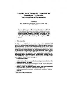
LR is calculated by dividing the heights of H0 and H1 distributions at the point of E (Fig. 1).
Figure 1: P (E|H0 ) and P (E|H1 ) for a given value of E. LR is the ratio of the heights of A and B points. LR is a measure widely used in many fields in forensic science. Since LR is calculated as a ratio of two heights, its estimation is sensitive to the mathematical modelling of the probability density function (pdf) of H0 and H1 and artifacts (especially in the tails of the pdf) can lead to erroneous estimation of LR. Very high scores of E are not often observed in the distribution of scores of H0 . In such a range of values the likelihood ratio declines despite the fact that such high scores are strong support for the hypothesis in which the two voices were produced by the same speaker. The phenomenon is related to the fact that the variance of the H1 distribution is bigger than the variance of the H0 distribution. As a consequence, this may lead to two different scores having the same LR. In Fig. 2 we see the evolution of the LR with respect to the score of E; an example is given for LR=5, to which two different scores correspond (see points S1 and S2).
In such a case it would mean that two different suspects may obtain the same LR despite the fact that one of them has a higher evidence score than the other. For both suspects the strength of the evidence is the same but for one of them the similarity between his voice and the questioned record, is higher. 4.2. Error Ratio We propose to use a second measure, the Error Ratio (ER), which contains complementary information to the strength of evidence (LR). This measure takes into consideration the relative risk of error for an obtained score, in choosing either of the hypotheses. ER is the ratio between the two types of errors, FNMR (False Non Match Rate) and FMR (False Match Rate) if the score E is used as a decision point. In other words, ER is the proportion of cases for which recordings from the same source would be wrongly considered to come from different sources, divided by the proportion of cases in which recordings from different sources were wrongly considered to be from the same source, if E is used as a threshold in a hypothesis test for match or non match (see Fig. 3):
ER =
P (N onM atch|H0 , E) F N M RE = P (M atch|H1 , E) F M RE
(2)
If the score of the trace given the suspect model is E, then error ratio (ER) is: RE p(x|H0 )dx (3) ER = R−∞ ∞ p(x|H 1 )dx E For example, for a given value of E, an ER of 10 means that the risk of making an error by excluding a suspect is ten times higher than the risk of identifying him as the source, if the score of E is used to decide. Note that although the DET (Detection Error Tradeoff) curve [13] shows the relative evolution of False Match with False Non Match probabilities, it cannot be used to estimate the extent of relative risk of error for a given E, since the score doesn’t appear implicitly in the plot and hence DET is useful only for the comparison and evaluation of system performance [14]. In the DET curve it can be remarked that False Alarm probability corresponds to the False Match Rate and the Miss probability corresponds to the False Non Match Rate.
Figure 3: The light gray area corresponds to the numerator of the ER (F N M RE ), the dark gray one to the denominator of the ER (F M RE ). Figure 2: First graph shows H0 and H1 score distributions and second graph shows LR evolution in which we can observe the same LR for two different scores of E.
Let us examine how the ER is calculated and what it means. The numerator of the ER corresponds to the area under the H0
distribution curve below E. This refers to the percentage of comparisons with a score smaller than the score E in which the source of the two compared recordings is the same. With the increase of the score of E (moving along the match score axis), the higher this percentage is, the lower the risk is in deciding in favor of the hypothesis H0 . In fact, if there are more comparisons between pairs of recordings (having the same source) giving a smaller score than E, it implies that the E of the case is actually a strong match. Similarly, the denominator of the ER is the area under the H1 curve above the score of E. It is the proportion of comparisons which have obtained a greater score than E for which the source of the two compared recordings is not the same. As this proportion of cases increases, so does the support for choosing H1 and the risk involved in choosing H0 is higher. Again, with the increase of the score of E, we come to the point where there are only very few comparisons between recordings coming from different sources giving a higher score than E, and the conviction that our value does not belong to the H1 distribution becomes stronger. Actually, if no comparison between recordings coming from different sources has given a value higher than E, this supports the hypothesis that E belongs to H0 distribution. If the decision threshold in a speaker verification system is set to E, the system cannot determine whether this trace comes from the suspect or not. This means that, for this particular case, the verification system would neither accept nor reject H0 . This is forensically desirable as at this threshold E no binary decision has to be made for the case. However, the expert can evaluate how good E would be as a decision threshold for similar cases for which he knows whether H0 or H1 is true. If the expert tries to evaluate the performance of a system based on this threshold (E) with all the cases in his experience to be similar to the given case, he will be able to obtain the False Match Rate and False Non Match Rate for this value of E. If he obtains a very high FMR and a very low FNMR, he knows that the risk involved in supporting the H0 hypothesis would be high. Similarly, if he obtains a low FMR and a high FNMR, implying a high ER, he can conclude that, based on his experience with cases under similar conditions, there is lower risk involved in accepting H0 . From the perspective of making a decision, it is desirable to know the relative risk of choosing one hypothesis over the other based on past experience with cases in similar conditions, using this system. Both the likelihood ratio and the error ratio present complementary information and we do not suggest the exclusive use of one method or the other. When LR=1 the probability of observing the score of E given one hypothesis (H0 ) is the same as given the competitive hypothesis (H1 ). The strength of evidence is one, and neither of the hypotheses can be favored. When the total error (FMR+FNMR) is minimum, it implies that at this point LR=1. ER, at this point, can be different from 1, since the risk of error that we would have if we took a decision in favor of one hypothesis might be higher than the risk of error taking a decision in favor of the other hypothesis. ER will be equal to 1 when, for a given value of E, the risk of error in choosing either of the hypotheses is equal.
5. Experimental Results In this section, we examine the evolution of ER and LR for different cases. This is performed applying the presented methodology and by means of a database which contains recordings in different conditions. In our experiments we have used the ASPIC (Automatic Speaker Identification by Computer) system, developed by EPFL and IPS-UNIL at Lausanne (Switzerland). ASPIC is a text-independent automatic speaker recognition system. The feature extraction is performed using RASTA PLP method and the statistical modelling is Gaussian Mixture Modelling. The database used is a subset of Polyphone IPSC02. The experiments were performed with a set of 10 speakers speaking German and French, and using a fixed phone as well as a cellular phone (GSM). The SR and SDB used are in French and in fixed telephone condition. Three situations are studied in which QR and TDB are: 1) French language and fixed phone 2) German language and fixed phone 3) French language and cellular phone. For each situation we have 5 utterances from each of these speakers for training their models (SDB), and 3 utterances that are used for testing (TDB). This means that we calculate scores for 150 H0 and for 1350 H1 cases, for each situation. The number of samples in each hypothesis is sufficient to generate probability density distributions for H0 and H1 scores. Figs 4, 5 and 6 present H0 and H1 score distributions for each of the three situations and the evolutions of the LR and the ER, first in a linear scale then in a logarithmic scale. Fig. 7 shows the compared DET curves for all the situations considered.
Figure 4: French Fixed SDB vs French Fixed TDB (situation 1). F M RE + F N M RE = minimum => LR = 1 F M RE = F N M RE f or ER = 1
(4) (5)
It is important to note that the evolution of the two measures
Figure 5: French Fixed SDB vs German Fixed TDB (situation 2).
Figure 6: French Fixed SDB vs French cellular (GSM) TDB (situation 3).
is different. While the LR after reaching a maximum begins to decrease (for such distributions), the ER continuously increases with the increasing of the score. We also notice that there are no significant differences between situations 1 and 2 (shown in Figs 4 and 5) where the only change concerns the language and a difference is observed with Fig. 6 when two different phone lines (fixed phone and cellular) were compared. The greater influence of technical mismatch compared to language mismatch can be observed in our experiments. The difference in performance of the automatic recognition system in these two different mismatched situations can be seen in Fig. 7.
6. Discussion The proposed methodology assumes that conditions in case recordings and database recordings are similar i.e., (TDB similar to QR and SDB similar to SR). Unfortunately, recording conditions in real cases are not always known and even with known conditions not always it is possible to obtain a database with identical (or very similar) conditions. It is possible however, that the expert collaborates with the investigation and performs the acquisition of both suspect data as well as the recordings required to create the comparison databases (SDB and TDB) in similar conditions. An interesting point of the methodology is that we can create in advance the probability distributions for H0 and H1 cases in different possible conditions, and evaluate a new case in the light of its corresponding conditions [15]. It will be necessary to determine whether the conditions of the database and the case are indeed compatible. The two interpretation measures, LR and ER, cannot be used instead of each other as they have different meanings and
Figure 7: DET curve for the three studied situations.
different evolutions although log of ER is similar to log of LR in some regions [16]. In the presented score-based system, in which the bigger the score is, the stronger the match is, we notice that the ER is a measure that increases as the score of E increases. ER gives in-
formation about the quality of the match for the obtained score. LR considers instead how many times you have observed the given value of E under the two hypotheses. If for a high value of E such a score is observed rarely in H0 cases, P (E|H0 ) will be very low, and so will the numerator of the LR. For the ER numerator, we are looking instead at every H0 case in which the score was smaller than E. So, although the given value of E is so high that it is rare, the numerator of ER will be very big. An advantage of using probabilities calculated using areas like in ER, over LR which uses likelihoods calculated by heights, is that mathematical artifacts are considerably reduced. Language mismatch (between train and test data) does not significantly affect the performance of the system in our experiments. Instead, the mismatch introduced by differences between fixed and cellular phone reduce drastically the performance.
7. Conclusion In this paper a general interpretation framework to handle forensic cases of automatic speaker recognition, where only one recording for the suspect is available, was presented. The assumptions needed in order to deal with such a framework and how to handle new cases were described. When suspect data is limited, the within-source variability of individual speakers can be approximated by the average within-source variability from representative databases. Normalization techniques should be used in order to reduce the bias due to mismatched recordings conditions [7]. Two measures for the interpretation of the evidence - the likelihood ratio (LR) and the error ratio (ER) - were presented and analyzed under different test conditions. Their comparative evolution with respect to the evidence is shown in different experiments. The weaker influence of language than technical conditions (cellular compared to fixed phone) on performance was observed in the experiments. While LR measures the strength of the evidence, ER gives complementary information to LR, about the quality of the match in a score-based framework (given the case and the databases), to interpret the observed value of the evidence. LR and ER cannot be used instead of each other as they have different meanings and different evolutions. The use of ER in the legal framework has to be investigated further.
8. Acknowledgments The authors would like to thank Quentin Rossy for his help in creation of the IPSC02 Polyphone database which has been used in the experiments in this paper.
9. References [1] F. Botti, A. Alexander, and A. Drygajlo, “Evaluation of Evidence in Forensic Speaker Recognition with a Questioned Recording and a Single Suspect’s Recording,” in 2003: Third European Academy of Forensic Science, Istanbul, Turkey, 2003. [2] C.G.G. Aitken, Statistics and the Evaluation of Evidence for Forensic Scientists, John Wiley & Sons, 1997. [3] A. Drygajlo, D. Meuwly, and A. Alexander, “Statistical Methods and Bayesian Interpretation of Evidence in Forensic Automatic Speaker Recognition,” in Proc. Eurospeech 2003, Geneva, Switzerland, 2003, pp. 689–692.
[4] D. Meuwly, M. El-Maliki, and A. Drygajlo, “Forensic Speaker Recognition Using Gaussian Mixture Models and a Bayesian Framework,” in 8th COST 250 workshop: Speaker Identification by Man and by Machine: Directions for Forensic Applications, 1998, pp. 52–55. [5] D. Meuwly, Reconnaissance de locuteurs en science forensiques: l’apport d’une approche automatique, Ph.D. thesis, University of Lausanne, 2001. [6] D. Meuwly and A. Drygajlo, “Forensic Speaker Recognition Based on a Bayesian Framework and Gaussian Mixture Modelling (GMM),” in 2001: A Speaker Odyssey, The Speaker Recognition Workshop, Crete, Greece, 2001, pp. 145–150. [7] A. Alexander, F. Botti, and A. Drygajlo, “Handling Mismatch in Corpus-Based Forensic Speaker Recognition,” in Proceedings of 2004: A Speaker Odyssey, Toledo, Spain, 2004, to be published. [8] D. A. Reynolds, “Comparison of Background Normalization Methods for Text-independent Speaker Verification,” in Proc. Eurospeech ’97, Rhodes, Greece, 1997, pp. 963– 966. [9] G. R. Doddington, W. Liggett, A. F. Martin, M. Przybocki, and D. A. Reynolds, “Sheep, Goats, Lambs and Wolves: A Statistical Analysis of Speaker Performance in the NIST 1998 Speaker Recognition Evaluation,” in International Conference on Spoken Language Processing, Sydney, Australia, November 1998. [10] R. Auckenthaler, M. J. Carey, and H. Lloyd-Thomas, “Score Normalisation for Text-independent Speaker Verification System,” Digital Signal Processing (DSP), a review journal - Special issue on NIST 1999 Speaker Recognition Workshop, vol. 10 (1-3), 2000. [11] D. A. Reynolds, T. F. Quatieri, and R. B. Dunn, “Speaker Verification using adapted Gaussian Mixture Models,” Digital Signal Processing, vol. 10, no. 1-3, pp. 19–41, 2000. [12] J. Navr´atil and G. N. Ramaswamy, “The Awe and Mystery of T-norm,” in Proc. Eurospeech 2003, Geneva, Switzerland, 2003, pp. 2009–2012. [13] A. Martin, G. Doddington, T. Kamm, M. Ordowski, and M. Przybocki, “The DET Curve in Assessment of Detection Task Performance,” in Proc. Eurospeech ’97, Rhodes, Greece, 1997, pp. 1895–1898. [14] H. Nakasone and S.D. Beck, “Forensic Automatic Speaker Recognition,” in 2001: A Speaker Odyssey, Crete, Greece, 2001, pp. 139–144. [15] J. Koolwaaij and L. Boves, “On Decision Making in Forensic Casework,” Forensic Linguistics, the International Journal of Speech, Language and the Law, vol. 6, no. 2, pp. 242–264, 1999. [16] B. Pfister and R. Beutler, “Estimating the Weight of Evidence in Forensic Speaker Verification,” in Proc. Eurospeech 2003, Geneva, Switzerland, 2003, pp. 701–704.