Software Tools for Technology Transfer manuscript No. (will be inserted by the editor)
An Interval-based SAT Modulo ODE Solver for Model Checking Nonlinear Hybrid Systems Daisuke Ishii1 , Kazunori Ueda1,2 , Hiroshi Hosobe2 1
2
Dept. of Computer Science, Waseda University 3-4-1, Okubo, Shinjuku-ku, Tokyo 169-8555, Japan e-mail: {ishii, ueda}@ueda.info.waseda.ac.jp National Institute of Informatics 2-1-2, Hitotsubashi, Chiyoda-ku, Tokyo 101-8430, Japan e-mail:
[email protected]
The date of receipt and acceptance will be inserted by the editor
Abstract. This paper presents a bounded model checking (BMC) tool called hydlogic for hybrid systems. It translates a reachability problem of a nonlinear hybrid system into a predicate logic formula involving arithmetic constraints, and checks the satisfiability of the formula based on a satisfiability modulo theories (SMT) method. We tightly integrate (i) an incremental SAT solver to enumerate the possible sets of constraints and (ii) an interval-based solver for hybrid constraint systems (HCSs) to solve the constraints described in the formulas. The HCS solver verifies the occurrence of a discrete change by enclosing continuous states that may cause the discrete change by a set of boxes. We adopt the existence property of a unique solution in the boxes computed by the HCS solver as (i) a proof of the reachability of a model, and (ii) a guide in the over-approximation refinement procedure. Our hydlogic implementation successfully handled several examples including those with nonlinear constraints.
1 Introduction One of the challenging problems in software verification is to design and analyse systems in which computer programs reliably interact with their physical environment [17]. Such systems are modeled as hybrid systems (Section 2.2) that consist of discrete and continuous changes over time. To develop reliable embedded controllers such as those for automobiles, we need to describe the specification as hybrid systems, and to prove the correctness of the systems. This paper is intended to construct a model checking tool for hybrid systems to verify the reachability to unsafe states. Tools for hybrid systems such as [10,15, 5, 16] have difficulties in modeling and verification, especially when the models belong to the class of
nonlinear hybrid systems, where vector fields in the continuous state space or conditions for discrete changes are expressed by nonlinear constraints. Since the above tools take linear hybrid systems as inputs, users need to linearize a problem by hand for each instance. In this paper, we propose a satisfiability modulo theories (SMT) framework for the bounded model checking (BMC) of nonlinear hybrid systems. In the BMC of hybrid systems, the bounded execution of a model is described by a predicate logic formula involving arithmetic constraints [1, 4, 3, 9]. Checking the satisfiability of the formula may become possible for systems that are too large for unbounded execution. An SMT solver enumerates propositional models of the formula using a SAT (propositional satisfiability) solver and then checks the consistency of these models by calling theory solvers that handle the conjunctions of arithmetic constraints. BMC for possibly nonlinear hybrid systems is simply encoded using formulas involving ordinary differential equations (ODEs) [3]. However, no existing implementations support nonlinear hybrid systems. Due to the state space explosion in handling the continuous state space of hybrid systems, abstraction methods play a significant role in model checking. Techniques for over-approximating state space by a set of boxes (tuples of intervals) [15, 4, 3] and polytopes [5] have been developed. In this paper, we use interval arithmetic (Section 2.1) for rigorous over-approximation. As a theory solver, we adopt a technique for hybrid systems proposed in our previous work [11] that integrates an interval-based method for nonlinear ODEs [13] and an interval-based constraint programming framework [8]. These interval-based methods guarantee that computed intervals or boxes enclose the solutions of a given problem. Moreover, the interval Newton methods guarantee that a unique solution exists in the computed intervals or boxes.
2
Daisuke Ishii et al.: An Interval-based SAT Modulo ODE Solver for Model Checking Nonlinear Hybrid Systems
More specifically, this paper presents a BMC tool for nonlinear hybrid systems called hydlogic. – hydlogic encodes a hybrid system into a predicate logic formula involving ODEs (Section 3). We describe a phase of continuous changes between two discrete changes as a hybrid constraint system (HCS) (Section 2.3) [11]. – We propose a set of algorithms for checking the satisfiability of the encoded formula (Section 4). The algorithms work tightly with (i) a SAT solver that enumerates possible sets of constraints, and (ii) a theory solver based on the HCS solver that simulates a phase of continuous change, i.e., computation of an initial value problem based on interval arithmetic. – In the proposed algorithms, the theory solver efficiently computes a set of boxes that enclose a counterexample by using the interval Newton method. Ordinary over-approximation methods do not necessarily guarantee that the computed enclosure contains a counter-example. In contrast, as a by-product of employing the interval Newton method, the HCS solver we adopt guarantees the existence of a unique solution in a result when the checking of certain conditions succeeds. This work focuses on the search of such sets of boxes in which a unique counter-example exists. When the algorithms fail to find such sets of boxes, we can still prove that the model has no counter-example by exhaustively searching the rest of the state space. We have implemented the hydlogic tool (Section 5) and used it to analyze several examples including those with nonlinear constraints (Section 6). 1.1 Related Work Eggers et al. [3] used an interval-based solver for ODEs in an SMT framework. However, their method did not support either nonlinear ODEs or nonlinear guard constraints which our method does. Their method was also limited in the integration with the SMT framework. The method collects ODEs and solves them in a round-robin manner. Our method solves ODEs incrementally while the SMT framework unrolls an execution path. To certify the result and to reduce the search space, our method utilizes the existence property of a unique solution obtained by the interval-based solver. Ratschan et al. [15] proposed to translate a safety verification problem of a hybrid system into a constraint satisfaction problem. They also provided an intervalbased implementation of the method that supports nonlinear constraints. Their method is not an SMT framework but is based on a specific set of complex constraints. Our method provides a simpler and more modular SMT framework that uses generic solvers for (nonlinear) equations and ODEs.
2 Preliminaries This section introduces notions used for describing the technique we propose. 2.1 Interval Arithmetic The proposed method is based on interval arithmetic [12]. A (bounded) interval [l, u] (l, u ∈ R) is a set of real numbers, where [l, u] = {r ∈ R | l ≤ r ≤ u}. I denotes a set of intervals. A box is a tuple (I1 , . . . , In ) of n intervals. In denotes a set of boxes. For an interval I ∈ I, lb(I) and ub(I) denote the lower and upper bounds, respectively. For a tuple X, X.i denotes the i-th component of X. For f : Rm → Rn , F : Im → In is called an f ’s interval extension iff it satisfies the following condition: ∀I1 ∈ I · · · ∀Im ∈ I ∀r1 ∈ I1 · · · ∀rm ∈ Im ∀i ∈ {1, . . . , n} [f (r1 , . . . , rm ).i ∈ F (I1 , . . . , Im ).i]. In the implementation of the proposed method, we use a machine-representable interval I such that lb(I) and ub(I) belong to a set of floating-point numbers F ⊂ R. In the computation of interval extensions, we handle the bounds of intervals rigorously to enclose the theoretical solutions and the accumulation of round-off errors. 2.2 Hybrid Systems Hybrid systems are systems consisting of discrete changes and continuous changes over time. We consider a reachability problem that decides whether the execution of a hybrid system may reach (or never reach) an unsafe state that is predetermined by the users. Definition 1. A hybrid system with unsafe states is a tuple HS = (Q, X , E, F, I, G, R, Init, US ) consisting of the following components: – – – – – –
– – –
A finite set Q of discrete states; A set X = Rn of continuous states; A finite set E ⊆ Q × Q of discrete state transitions; A family F = {fq }q∈Q of vector fields fq : X → Rn . We assume fq is a Lipschitz continuous function; A family I = {Inv q }q∈Q of invariants Inv q = I1 × · · · × In , where I1 , . . . , In ∈ I; A family G = {ge (x) = 0}e∈E of guard constraints, where x is a variable over X , and ge is a differentiable function X → R; A family R = {rst e }e∈E of (polynomial) reset functions rst e : X → X ; A set of initial states Init = (q0 , I1 × · · · × In ), where q0 ∈ Q and I1 , . . . , In ∈ I; A finite set US ⊆ Q of unsafe states. ⊓ ⊔
Daisuke Ishii et al.: An Interval-based SAT Modulo ODE Solver for Model Checking Nonlinear Hybrid Systems
A k-step execution of a hybrid system is an alternating sequence of discrete change phases (DPs) and continuous change phases (CPs) DP0
CP0
DP1
correct left p˙ = −r · sin(γ) γ˙ = ω c˙ = −2 −1 ≤ p ≤ 1 c≥0
−−−→ (q 0 , x0 , t0 ) −−−→ (q 0 , x1− , t1 ) −−−→ · · · DPk−1
CPk−1
−−−−→ (q k−1 , xk−1 , tk−1 ) −−−−→ (q k−1 , xk− , tk ), where: 0 i+1 – q i ∈ Q, xi , xi+1 ∈ R≥0 (i ∈ {0, . . . , − ∈ X , and t , t k−1}); – DP0 stands for the establishment of an initial state (q 0 , x0 , t0 ) ∈ Init; – For i ∈ {1, . . . , k−1}, DPi is an (instant) state transii+1 tion from (q i , xi+1 ) to (q i+1 , xi+1 , ti+1 ) at time − ,t ti+1 ∈ R≥0 , where (q i , q i+1 ) ∈ E, g(qi ,qi+1 ) (xi+1 − ) = 0, and xi+1 = rst (qi ,qi+1 ) (xi+1 ) hold; − – For i ∈ {0, . . . , k −1}, CPi is a continuous evolution of states from xi ∈ X to xi+1 ∈ X while a discrete − state q i is enabled.
Let 0 < t0 < · · · < tk−1 be k time points, q i a discrete state enabled over the time interval (ti , ti+1 ), fqi a vector field corresponding to q i , and xi ∈ X a continuous state at time ti . Then, a continuous function (or trajectory) y : [ti , ti+1 ] → X is determined with the ODE y(τ ˙ ) = fqi (y(τ )) ∧ y(ti ) = xi , where y(τ ˙ ) = dy(τ )/dτ . Since fqi is Lipschitz continuous, a unique trajectory is determined by the ODE. For all t ∈ [ti , ti+1 ], y(t) ∈ Inv qi holds. xi+1 is obtained as y(ti+1 ). In the following, we − call the pair (DPi , CPi ) the i-th step of an execution. For a hybrid system, a state q ∈ Q is reachable within k steps if and only if there exists a k-step execution where ∃i ∈ {0, . . . , k − 1}[qi = q]. A hybrid system is unsafe (resp. safe) within k steps if and only if there exists a state us ∈ US reachable (resp. unreachable) within k steps. Example 1. We describe a controller that steers a car along a straight road near a canal [2]. Figure 1 shows the controller modeled as a hybrid system. The model consists of 7 discrete states corresponding to each node, 3-dimensional continuous states (p, γ, c) ∈ R3 , and 9 discrete state transitions corresponding to each edge. Let p, γ, and c represent the horizontal position of the car, the heading angle, and the internal timer, respectively. A discrete state labeled go ahead has a vector field (−r · sin(γ), 0, 0) and an invariant [−1, 1] × [−∞, ∞] × [−∞, ∞]. The set of initial states is (go ahead, [−1, 1] × [−π/4, π/4] × [0]). A transition e from go ahead to left border has a guard constraint ge (x) = p + 1 = 0 and a reset function rst e (x) = (p, γ, 0) (x is a variable over R3 ). An edge entering go ahead represents the initial constraint. Reaching the state labeled in canal in an execution signals the unsafety of the model. ⊓ ⊔
c=0
straight ahead p˙ = −r · sin(γ) γ˙ = 0 c˙ = 0
p=1 c := 0
p = −1 left border p˙ = −r · sin(γ) γ˙ = −ω c˙ = 1 −1.5 ≤ p ≤ −1
p = −1 c := 0
go ahead p˙ = −r · sin(γ) γ˙ = 0 c˙ = 0 −1 ≤ p ≤ 1
c=0
3
correct right p˙ = −r · sin(γ) γ˙ = −ω c˙ = −2 −1 ≤ p ≤ 1 c≥0
p = −1 c := 0
p=1
p=1 c := 0
right border p˙ = −r · sin(γ) γ˙ = ω c˙ = 1 1≤p
p = −1.5 in canal p˙ = 0 γ˙ = 0 c˙ = 0
−1 ≤ p ≤ 1 −π/4 ≤ γ ≤ π/4 c=0
Fig. 1. Model of the car steering example.
2.3 Hybrid Constraint Systems We formulated the problem of detecting a discrete change in hybrid systems as a hybrid constraint system, consisting of a flow constraint on trajectories and a guard constraint on states causing discrete changes [11]. The solution to such a system is the crossing point(s) of a trajectory and a boundary in the state space represented by a guard constraint. Definition 2. A hybrid constraint system (HCS) is a tuple HCS = (˜ x, flow q , grd e , D, D0 ) with the following components: – A tuple of variables x ˜ = (x0 , x1 , . . . , xn ) consisting of a variable x0 representing the time x0 ∈ R≥0 at a crossing point and n variables x1 , . . . , xn representing a continuous state in X = Rn at time x0 ; – A flow constraint flow q (˜ x) corresponding to a discrete state q ∈ Q, which is described by the conjunction of the four equations flow q (˜ x) ≡ y(τ ˙ ) = fq (y(τ )) ∧ y(t0 ) = y0 ∧ y(x0 ) = (x1 , . . . , xn ) ∧ x0 > t0 , where t0 ∈ R≥0 , y0 ∈ X , y(τ ) is a trajectory [t0 , tmax ] → X ([t0 , tmax ] ∈ I); – A guard constraint grd e (x1 , . . . , xn ) corresponding to a transition e ∈ E is described by grd e (x1 , . . . , xn ) ≡ ge (x1 , . . . , xn ) = 0; – A domain D = (D0 , . . . , Dn ) ∈ In+1 that contains possible values of the variables; – An initial value set D0 = (D0,0 , . . . , Dn,0 ) ∈ In+1 that contains values for parameters t0 and y0 in flow q . ⊔ ⊓ The valuation of an HCS is a map of the form x ˜ 7→ (d0 , . . . , dn ) from every variable xi = x ˜.(i+1) to a value
4
Daisuke Ishii et al.: An Interval-based SAT Modulo ODE Solver for Model Checking Nonlinear Hybrid Systems
di ∈ Di . A solution of the HCS is a valuation satisfying the constraints flow q and grd e . An HCS may have multiple solutions. In [11], we proposed a technique for solving HCSs by coordinating (i) interval-based solving of nonlinear ODEs and (ii) a constraint programming technique for reducing interval enclosures of solutions. Our technique provides the following characteristics: (a) the computation is regarded as a contracting map SHCS : In+1 → n+1 2I , where ∀D′ ∈ SHCS (D)[D′ ⊆ D]; (b) the domain D′ ∈ SHCS (D) is box-consistent, i.e., for each bound b of a component Di of D′ , interval-based computation of constraints with a valuation x ˜ 7→ (D0 , . . . , [b], . . . , Dn ) encloses a solution of the HCS. The interval Newton method used in SHCS guarantees the existence property of computed intervals. SHCS checks certain conditions when applying the interval Newton method, and if the conditions hold, it guarantees that a unique solution exists in the computed domain for each value in the initial domain D0 . Example 2. Consider an execution in the discrete state q = go ahead ∈ Q of the model in Example 1, which will move to the state left border with e = (go ahead, left border) ∈ E. We can express the continuous state in q causing a discrete change with respect to e by an HCS consisting of the following components: x ˜ = (t, p, γ, c), flow q (˜ x) ≡ y(τ ˙ ) = (−r · sin(y(τ ).3), 0, 0) ∧ y(t0 ) = y0 ∧ y(t) = (p, γ, c) ∧ t > t0 , grd e (p, γ, c) ≡ p + 1 = 0, D = (R≥0 , [−1, 1], R, R), D0 = ([0], [−1, 1], [−π/4, π/4], [0]). The flow constraint flow q is parametrized by variables t0 and y0 that range over [0] and [−1, 1]×[−π/4, π/4]×[0], respectively. ⊓ ⊔ 3 Constraint-based Representation of Hybrid Systems We describe hybrid systems involving unsafe states as predicate logic formulas with flow and guard constraints described in Section 2.3. We propose how a reachability problem of a hybrid system is translated into satisfiability checking of a formula. This encoding method is a modification of the former methods [1,3]. Definition 3. A k-step execution of HS is encoded as a formula [[HS ]]k as follows. 1. Prepare the following variables: – (k + 1) Boolean variables biq (i ∈ {0, . . . , k}) for each discrete state q ∈ Q representing whether the state is activated in the i-th step;
– k Boolean variables bie (i ∈ {0, . . . , k−1}) for each discrete state transition e ∈ E representing the activation of the transition; – (k+1) variables xi (i ∈ {0, . . . , k}) and k variables xi− (i ∈ {1, . . . , k}) over n-real vectors representing the continuous state after the i-th transition and before the (i + 1)-st transition, respectively; – k variables ti over R≥0 (i ∈ {0, . . . , k−1}) representing the time at which the i-th transition takes place; – k variables xiinv over n-dimensional real vectors and k variables tinv over R≥0 (i ∈ {0, . . . , k−1}). 2. The following formulas express that a unique discrete state is activated and a unique transition takes place in the i-th step UQ i =
⊗
biq ,
q∈Q
UE i =
⊗
bie ,
e∈E
where ⊗ means that exactly one of the arguments is true. 3. The following formula expresses the CP corresponding to the discrete state q in the i-th step CONT i =
∧
(biq ⇒ flow iq (ti+1 , xi+1 − )).
q∈Q
The invariant in the i-th step is described through the following formula INV i =(flow iq (tiinv , xiinv ) ∧ ti ≤ tiinv ≤ ti+1 ∧ xiinv ∈ / Inv q ) ⇒ ¬biq . 4. Taking a discrete state transition e = (q, q ′ ) ∈ E at step i implies enabling the discrete states q at step i and q ′ at step i + 1. Moreover, the guard constraint should be satisfied by xi− , and the initial state xi+1 for the next step is determined by the reset function. For transitions in E, we describe the following formulas ∧ EDGE i = (bie ⇒ (biq ∧ bi+1 q ′ )), e=(q,q ′ )∈E
TRANS i =EDGE i ∧
∧
(bie ⇒ (grd e (xi− )
e∈E
∧ xi+1 = rst e (xi− ))). 5. Let q be a discrete state specified in Init.1. The initial state is described by the following formula INIT = b0q ∧ x0 ∈ Init.2. 6. Finally, conjunct all the formulas described above. We also express that the unsafety (to be falsified in model checking) holds. In this paper, unsafety properties are represented as discrete states US ⊆ Q in a model. For each variable bius corresponding to
Daisuke Ishii et al.: An Interval-based SAT Modulo ODE Solver for Model Checking Nonlinear Hybrid Systems
us ∈ US , we express that us will be reached within the k-step execution [[HS ]] =INIT ∧ k
k−1 ∧
(UQ i ∧ UE i ∧ CONT i ∧ INV i
i=0
∧ TRANS i ) ∧ UQ k ∧
k ∨ ∨
bius . ⊓ ⊔
i=0 us∈US
Proposition 1. For a hybrid system HS , suppose [[HS ]]k is a formula encoded for k steps as described above. If [[HS ]]k is unsatisfiable, then HS is safe for its k-step execution. ⊓ ⊔
4 Algorithms for Checking the Satisfiability In this section, we propose a set of algorithms for checking the satisfiability of the formula [[HS ]]k described in Section 3. We use interval-based techniques to deduce the satisfiability of constraints in a formula by computing a set of boxes that may enclose the solution of the constraints. As in DPLL(T ) [6], we tightly integrate a modern SAT solver and a theory solver, i.e., the HCS solver described in Section 2.3. Our method incrementally runs a SAT solver, for each step, to enumerate combinations of active constraints in a formula, such as the discrete state to enable in the current step, the flow constraint in the discrete state, and the guard constraint for a possible transition from the current state. Then, the interval-based HCS solver computes an enclosure of states causing the next discrete change. With this result, the algorithms check the consistency of the set of constraints for the current step. As in the previous work [2, 15, 4,3], we refine an overapproximation of continuous changes in a solving process to obtain a more accurate enclosure. Refinements are done by splitting one of the components of an initial boxed value. The refined initial values are enumerated by the SAT solver. In our method, refinements are guided by whether computed intervals are proved to enclose a unique solution, or whether by or an initial interval value is precise enough. 4.1 Incremental Solving The IncSolve algorithm illustrated in Figure 2 checks the satisfiability of the formula [[HS ]]k . Input to the algorithm is a hybrid system with unsafe states HS , and a maximum number of steps k ∈ N to verify. The algorithm returns one of the following values: Sat (satisfiable); Unsat (unsatisfiable); Unknown indicating that it cannot be decided whether the formula is satisfiable or not (due to the too coarse initial condition). When Sat is returned, the existence of a counter-example, which signals the unsafety of the systems, is guaranteed.
5
At lines 1–2, the algorithm translates HS into [[HS ]]k and reads the subformula Init describing the initial states into the proposition database P (P is always modified by appending formulas). When reading a predicate logic formula lf , the algorithm first translates lf into a propositional logic formula bf by mapping each constraint in lf to a propositional variable (these maps are preserved in a table), and then substitutes bf into P . A flag uk initialized in line 3 indicates whether the satisfiability of the formula can be decidable or not. In the loop starting from line 5, the algorithm incrementally checks the satisfiability of [[HS ]]i for i ∈ {0, . . . , k−1}. At line 6, the subformulas UQ i , CONT i , INV i , and EDGE i are read. Then the SAT solver processes the proposition P and computes a valuation for the propositional variables within them (lines 7–10). If there is no valuation, the algorithm terminates and returns Unknown or Unsat. Note that TRANS i is not handled here. The algorithm returns Sat if the current discrete state is unsafe (line 12). The decision of a transition e ∈ E to take place is computed in the HcsPropag procedure described in the next section (line 14). For each e ∈ E from the state q i , HcsPropag checks whether the transition will be enabled or not, and returns the result res e of the check, a reachable continuous state De that is consistent with the guard constraint grd e , and the next discrete state qe to proceed to. At lines 15–25, the algorithm analyzes the results. When the box De is guaranteed to contain a unique solution of grd e , the algorithm learns an initial condition for the next step and proceeds to the next loop (line 17). When grd e is unsatisfiable, the algorithm learns that it does not need to re-check this transition in the sequel (line 20). This is effective when the algorithm refines the initial domain and re-simulates the execution from the domain. Otherwise, grd e may be satisfied or may not. Thus, the algorithm tries to refine the initial domain (see Section 4.3) at line 23. If it cannot be refined, i.e., the initial domain is too coarse to divide, the algorithm turns on the flag uk . If there is no possible transition, the algorithm returns Unknown or Unsat (line 27). 4.2 Propagation by Solving HCSs The HcsPropag algorithm (Figure 3) computes a continuous state evolution simultaneously evaluating the guard constraints to determine the next transition to take place. This is done by constructing an HCS for each candidate transition, and solving it with the method described in Section 2.3. The procedure is equivalent to theory propagation in DPLL(T ). The input consists of a set E of candidate transitions, an initial domain D0 for the HCS, a flow constraint flow q for the current step, and an invariant Inv q . The destination state qe and the guard constraint grd e are given by a transition e ∈ E (line 3). At line
6
Daisuke Ishii et al.: An Interval-based SAT Modulo ODE Solver for Model Checking Nonlinear Hybrid Systems
Input: a hybrid system HS , and a maximum step k Output: satisfiability sat ∈ {Sat, Unsat, Unknown} 1: encode HS to obtain [[HS ]]k 2: P := INIT 3: uk := false 4: i := 0 5: while 0 ≤ i ≤ k−1 do 6: P := P ∧ (UQ i ∧ UE i ∧ CONT i ∧ INV i ∧ EDGE i ) 7: sat := Solve(P ) 8: if ¬sat then 9: return uk ? Unknown : Unsat 10: (q i , D0i , flow iqi , Inv q ) := collect true-valued constraints from P 11: if q i ∈ US then 12: return Sat 13: E ′ := {(q, q ′ ) ∈ E | q = q i } 14: {(res e , De , qe )}e∈E ′ := HcsPropag(E ′ , D0i , flow iqi , Inv q ) 15: for e ∈ E ′ do 16: if res e = true then 17: P := P ∧ ((q i+1 = qe ) ⇒ (xi+1 ∈ Rst e (De ))) 18: else 19: if De = ∅ then 20: P := P ∧ (¬e) 21: else 22: if ¬ (the initial domain is precise enough) then 23: P := Refine(P ); i := 0; Continue() 24: else 25: uk := true; P := P ∧ (¬e) 26: i := i + 1 27: return uk ? Unknown : Unsat Fig. 2. IncSolve algorithm.
4, an initial domain is prepared by setting a maximum time interval beyond the initial time and the invariant box for the current state. An HCS is solved at line 5 and a set of box-consistent domains are obtained as a result. Domains in the set are enumerated at lines 6–13. As described in Section 2.3, the SHCS we adopt may guarantee that a resulting domain contains a unique solution with respect to every initial value in D0 . The algorithm returns true if the existence of a solution is guaranteed, or false otherwise. 4.3 Over-approximation Refinement The Refine procedure called in IncSolve tries to refine an over-approximation by dividing the initial box and re-computing the over-approximation for each of the divided boxes. In a refinement, an initial box is divided along one of the components of the box (each time the component is changed in a round-robin manner). Each time an initial box is refined, the solver learns an additional formula on the initial constraint. In the formula, we use Boolean variables id i (i ∈ N) which give an identifier to each initial box. Beforehand, we give id 0 to INIT by adding the formula id 0 ⇔ INIT to the proposition
Input: a set E of transitions, an initial domain D0 , a flow constraint flow q , and an invariant Inv q Output: a set R of tuples (res, D, q), where res ∈ {true, false}, D ⊆ X , and q ∈ Q 1: R := ∅ 2: for e ∈ E do 3: (qe , grd e ) := collect the destination state and the guard constraint of e 4: D := (D0 , . . . , Dn ), where D0 = [lb(D0 .1), tmax ] and D1 × · · · × Dn = Inv q 5: DS := SHCS (D), // see Section 2.3 where HCS = (˜ x, flow q , grd e , D, D0 ) 6: if DS = ∅ then 7: R := R ∪ {(false, ∅, qe )} 8: else 9: for D ∈ DS do 10: if D is proved to contain a solution then 11: R := R ∪ {(true, D, qe )} 12: else 13: R := R ∪ {(false, D, qe )} 14: return R Fig. 3. HcsPropag algorithm.
database P . Let D0 be an initial boxed value, and assume that D0 is divided into boxes D0,1 and D0,2 . Then, we construct the following formula and add this to the solver. ((id 0 ∧ q i+1 ) ⇒ (id 1 ⊕ id 2 )) ∧ (¬id 1 ∨ ¬id 2 ) ∧ (id 1 ⇒ (x0 ∈ D0,1 )) ∧ (id 2 ⇒ (x0 ∈ D0,2 )). After a refinement, the Continue() command at line 23 of IncSolve restarts the solving loop from step i = 0. Accordingly, one of the identifiers id 1 and id 2 is selected, and the computation of refined over-approximation starts. Note that not id 1 and id 2 but id 0 may be selected because a search along a different path may be still on the way. 4.4 An Example We describe how the proposed method verifies the hybrid system in Example 1. Here, we change the initial domain to (p, γ, c) ∈ [−1, 0]×[π/6, π/4]×[0]. Parameters are set as r = 2 and ω = π/4. Computed domains for p along the time line are illustrated in Figure 4. Enumeration of refined initial domains and decisions on transitions are illustrated in Figure 5. The computation proceeds as follows: a. At line 10 of IncSolve, the initial state go ahead and the initial domain D0 = ([0, tmax ], [−1, 0], [π/6, π/4], [0]) is activated using the SAT solver (we denote D0 by D0,0 in the following, where the identifier for (refined) domains is subscripted). Then, HcsPropag constructs HCSs with respect to the state go ahead and the transitions from go ahead to left border and right border. By solving these, HcsPropag
Daisuke Ishii et al.: An Interval-based SAT Modulo ODE Solver for Model Checking Nonlinear Hybrid Systems
Fig. 4. Process of solving the car steering example. The horizontal line at t = 0 denotes the initial domains for p. The vertical lines are the boundary values at the discrete state transitions. In (a), the p component of the domain is divided into two (D0,1 and D0,2 ). In (b), the γ component is divided (D0,3 and D0,4 ). Bending lines show the results of numerical computation using the boundary values of the initial domain.
0
1
(true, D0,0 , go ahead)
(false, D1,0 , left border)
id \ step
0
2
3
(false, ∅, right border)
1
(true, D0,1 , go ahead)
(true, D1,1 , left border)
(false, D2,0 , in canal)
(true, D2,1 , correct left)
2
(true, D0,2 , go ahead)
(false, D1,2 , left border)
3
(true, D0,3 , go ahead)
(true, D1,3 , left border)
(false, D2,2 , in canal)
4
(true, D0,4 , go ahead)
(true, D1,4 , left border)
(true, D2,3 , in canal)
(true, D3,0 , straight ahead)
(false, ∅, right border)
Fig. 5. Enumeration of possible execution paths. Enumeration starts from the upper-left of the figure. A simulation from an initial domain proceeds horizontally as directed by the arrows. Each node is a tuple of a result of evaluating a guard constraint, a domain satisfying the guard constraint, and the next state to transit. Refinements of the initial domains are shown by the identifier numbers directed by the dotted arrows.
computes the results {(false, D1,0 , left border), (false, ∅, right border)}. Since all the results contain false, the algorithm refines D0,0 to D0,1 and D0,2 by dividing the component [−1, 0] for p into [−0.5, 0] and [−1, −0.5]. b. Afterward, HcsPropag computes the result {(true, D1,1 , left border)} from D0,1 . IncSolve proceeds to step 1 of the execution, and HcsPropag com-
7
putes the results {(false, D2,0 , in canal), (true, D2,1 , correct left)} from D1,1 . Since D2,0 is returned with false, D0,1 is refined into D0,3 and D0,4 along the component for γ, i.e., [π/6, π/4] into [π/6, 5π/24] and [5π/24, π/4]. The algorithm also computes the execution path that moves to correct left at step 2, and reaches straight ahead at step 3. c. From D0,2 , the algorithm is still unable to decide whether the transition to left border may be enabled or not. The algorithm applies another refinement. d. From D0,3 , the algorithm computes the results without the guarantee of existence, as in the computation from D0,1 . Note that the path to straight ahead is not computed here again, since the existence of this path is learned in Step b. e. Finally, from D0,4 , the algorithm computes a counterexample guaranteed to reach in canal at step 2. 5 Implementation We built a prototype implementation called hydlogic of the method described in this paper. hydlogic is implemented in OCaml, C, and C++, and consists of about 2000 lines of code. Input to hydlogic is a textual description of a hybrid system. hydlogic translates an input model into a formula as explained in Section 3. Then, the core component checks the satisfiability of the formula by the method in Section 4. hydlogic integrates the following external solvers. – The Decision Procedure Toolkit (DPT) [7] is used as an incremental SAT solver. DPT is an implementation of a DPLL-based SAT solver in OCaml. It has a flexible API for adding clauses incrementally and controlling search procedures. – We use the implementation described in [11] for solving HCSs. The HCS solver is built on top of Elisa [8], an interval-based constraint solver based on boxconsistency, and VNODE-LP [13], which handles initial value problems for ODEs based on interval arithmetic. The whole system is implemented in C++. 6 Experiments We present results of experiments on three examples. It shows how the complexity scales by the unrolled execution steps, the size of models, and the size of boxes given by initial constraints. We also compared the tool with HSolver [15] and PHAVer [5]. We experimented on a 2.4GHz Intel Core 2 Duo processor with 4GB of RAM. 6.1 Car Steering Problem Consider the car steering problem given in Example 1. We first analyzed the unsafety of the model as described
8
Daisuke Ishii et al.: An Interval-based SAT Modulo ODE Solver for Model Checking Nonlinear Hybrid Systems
in Section 4.4. hydlogic took 692.74 seconds and 1716 times of refinements to prove the existence of a counterexample. We set the minimum width wmin of the initial boxed values to 0.05, and the time domain D.1 in the HCSs to [0, 3]. We then modified the guard constraint for the edge entering in canal as p = 2, and analyzed the model again. hydlogic returned the result Unknown in 91.88 seconds. Refinements were done 48 times. The result was Unknown because it was unable to prove the existence property for some of the guard constraints and the initial values. For example, when the initial domain for p was [0, 0.05], the existence of a solution to the guard constraint of left border was not proved. We confirmed that all the evaluation of the transition to in canal had no solution. We tried to solve the same instance of this problem by HSolver but the computation did not terminate after 10 minutes (though HSolver could solve another instance of the problem). 6.2 Navigation Benchmark We present results of the navigation benchmark problem taken from [5,15]. This problem models an object at a position (px (t), py (t)) ∈ R2 moving within a grid of n × n areas of size 1 × 1 (n ∈ N). Each area in the grid determines the velocity (vx (t), vy (t)) of the object as (v˙x (t), v˙y (t))T = A · ((vx (t), vy (t))T − vd ), where ( ) −1.2 0.1 A= , vd = (sin(i · π/4), cos(i · π/4))T . 0.1 −1.2 i ∈ {0, . . . , 7} is determined by each area. The lower left corner area of the grid has the coordinate (0, 0). We used U2 4 a map specified by the following matrix M = 4 3 4 , 2 2U where U denotes an unsafe region, and the other numbers indicate the values i of the corresponding areas. We set the initial discrete state as the (1, 2) area in the grid, and set the initial values as (px,0 , py,0 , vx,0 , vy,0 ) ∈ [0, 1] × [1, 2] × [0.5] × [0]. We analyzed the reachability to the unsafe areas using hydlogic. Parameters are set as k = 4, wmin = 0.25, and tmax = 10. We proved the existence of a path from the initial state, where (px,0 , py,0 ) ∈ [0.25, 0.5] × [1.5, 1.75], to the unsafe area at (3, 3). The analysis took 60.1 seconds and 34 refinements. We then modified the initial condition for py to py,0 ∈ [1, 1.5], and tried to find an execution path reaching to the unsafe area at (1, 1). We analyzed for k ∈ {2, . . . , 7} and each computation returned Unknown because there were some guard constraints not guaranteed to be satisfied. We confirmed those guard constraints are not for the boundary of the unsafe area. The computation took
37.93, 40.33, 43.46, 70.37, 70.36, and 70.38 seconds, respectively. PHAVer can check the safety of several instances of this problem [5]. An advantage of hydlogic is that it can prove the existence of a path reaching the goals specified as unsafe areas. As previously experimented [15], HSolver could not solve this problem. 6.3 Tunnel Diode Oscillator Circuit The third example taken from [5] models an RLC circuit involving a tunnel diode. The two dimensional continuous state (i, v) ∈ R2 expresses the current i through the inductor and the voltage drop v of the tunnel diode. The vector fields are specified as in the original paper. We describe the model as a hybrid system, where each discrete state corresponds to an equation for id . In the experimentation, we unrolled the model for 7 steps and tried to find a path. We set the initial constraint as taking q3 for the discrete state, and (i, v) ∈ [0.0006] × [0.45] for the continuous state. hydlogic computed an enclosure of a path with the guarantee of the existence. It took 4332 seconds. Most of the CPU time was spent by VNODE-LP to solve the ODEs because VNODE-LP can only take small time steps (around 10−8 ) in its iterative computation. In [5], PHAVer took a model, which is linearized beforehand, and proved that the continuous state stayed within a certain region. HSolver also solved a reachability problem based on this example in a reasonable time [15]. Our method might solve reachable sets more efficiently by applying recent techniques for solving ODEs with uncertain initial domains. By detecting that a box enclosure of a state in an execution is included in the initial domain, we can verify the safety for the infinite steps.
7 Conclusion We have presented the hydlogic tool for verifying systems that interact with physical environments. We provide hydlogic as an SMT-based tool that inter-works with an incremental SAT solver and an interval-based constraint solver. hydlogic supports nonlinear hybrid systems (Definition 1) involving nonlinear ODEs and nonlinear guard constraints, which cannot be handled by the most of the available tools. The proposed method utilizes the property to guarantee the existence of a unique solution in an over-approximation provided by the HCS solver. The property is used to prune the search space in the proposed algorithms, as well as to output a set of boxes in which a counter-example of a model (or a path to the goal) is guaranteed to exist.
Daisuke Ishii et al.: An Interval-based SAT Modulo ODE Solver for Model Checking Nonlinear Hybrid Systems
In this paper, refinement of an over-approximation is performed by simply dividing an initial box. The refinement method can be improved in several ways using techniques for handling nonlinear ODEs with uncertainties [14], for example. Acknowledgements. The authors are indebted to anonymous referees for their useful comments. The authors are also indebted to the members of the HydLa project for the development of the ideas. This research is partially supported by JSPS, Grant-in-Aid for Young Scientists (B) 20700033 and Grant-in-Aid for Scientific Research (B) 20300013.
References 1. G. Audemard, M. Bozzano, A. Cimatti, and R. Sebastiani. Verifying industrial hybrid systems with MathSAT. Electronic Notes in Theoretical Computer Science, 119(2):17–32, 2005. 2. E. Clarke, A. Fehnker, Z. Han, B. Krogh, O. Stursberg, and M. Theobald. Verification of hybrid systems based on counterexample-guided abstraction refinement. In Proc. of TACAS’03, LNCS 2619, pp. 192–207, 2003. 3. A. Eggers, M. Franzle, and C. Herde. SAT modulo ODE: A direct SAT approach to hybrid systems. In Proc. of ATVA’08, LNCS 5311, pp. 171–185, 2008. 4. M. Fr¨ anzle, C. Herde, T. Teige, S. Ratschan, and T. Schubert. Efficient solving of large non-linear arithmetic constraint systems with complex boolean structure. Journal on Satisfiability, Boolean Modeling and Computation (JSAT), 1:209–236, 2007. 5. G. Frehse. PHAVer: Algorithmic verification of hybrid systems past HyTech. International Journal on Software Tools for Technology Transfer (STTT), 10(3):263–279, 2008. 6. H. Ganzinger, G. Hagen, R. Nieuwenhuis, A. Oliveras, and C. Tinelli. DPLL(T): Fast decision procedures. In Proc. of CAV’04, LNCS 3114, pp. 175–188, 2004. 7. A. Goel and J. Grundy. Decision Procedure Toolkit 1.2. http://dpt.sourceforge.net/, 2008. 8. L. Granvilliers and V. Sorin. Elisa 1.0.4. http://sourceforge.net/projects/elisa/, 2005. 9. S. Gulwani and A. Tiwari. Constraint-based approach for analysis of hybrid systems. In Proc. of CAV’08, LNCS 5123, pp. 190–203, 2008. 10. T. J. Hickey and D. K. Wittenberg. Rigorous modeling of hybrid systems using interval arithmetic constraints. In Proc. of HSCC’04, LNCS 2993, pp. 402–416, 2004. 11. D. Ishii, K. Ueda, H. Hosobe, and A. Goldsztejn. Interval-based solving of hybrid constraint systems. In Proc. of the 3rd IFAC Conference on Analysis and Design of Hybrid Systems (ADHS’09), pp. 144–149, 2009. 12. R. E. Moore, R. B. Kearfott, and M. J. Cloud. Introduction to Interval Analysis. SIAM, 2009. 13. N. S. Nedialkov. VNODE-LP: a validated solver for initial value problems in ordinary differential equations. TR CAS-06-06-NN, McMaster University, 2006. 14. N. Ramdani, N. Meslem, and Y. Candau. A hybrid bounding method for computing an over-approximation for the reachable space of uncertain nonlinear systems. IEEE Trans. on Automatic Control, 2009 (to appear).
9
15. S. Ratschan and Z. She. Safety verification of hybrid systems by constraint propagation-based abstraction refinement. ACM Trans. on Embedded Computing Systems (TECS), 6(1), Article 8, 2007. 16. S. Sankaranarayanan, F. Ivancic, and T. Dang. Symbolic Model Checking of Hybrid Systems using Template Polyhedra. In Proc. of TACAS’08, LNCS 4963, pp. 188–202, 2008. 17. L. Sha, S. Gopalakrishnan, X. Liu, and Q. Wang. Cyberphysical systems: a new frontier. Machine learning in cyber trust: security, privacy, and reliability, pp. 3–14, Springer-Verlag, 2009.