An Interval Partitioning Approach for Continuous Constrained Optimization 2 ¨ Chandra Sekhar Pedamallu1 , Linet Ozdamar , and Tibor Csendes3 1
2 3
Nanyang Technological University, School of Mechanical and Aerospace Engineering, Singapore
[email protected] Izmir Ekonomi Universitesi, Izmir, Turkey
[email protected] University of Szeged, Institute of Informatics, Szeged, Hungary
[email protected]
Summary. Constrained Optimization Problems (COP’s) are encountered in many scientific fields concerned with industrial applications such as kinematics, chemical process optimization, molecular design, etc. When non-linear relationships among variables are defined by problem constraints resulting in non-convex feasible sets, the problem of identifying feasible solutions may become very hard. Consequently, finding the location of the global optimum in the COP is more difficult as compared to bound-constrained global optimization problems. This chapter proposes a new interval partitioning method for solving the COP. The proposed approach involves a new subdivision direction selection method as well as an adaptive search tree framework where nodes (boxes defining different variable domains) are explored using a restricted hybrid depth-first and best-first branching strategy. This hybrid approach is also used for activating local search in boxes with the aim of identifying different feasible stationary points. The proposed search tree management approach improves the convergence speed of the interval partitioning method that is also supported by the new parallel subdivision direction selection rule (used in selecting the variables to be partitioned in a given box). This rule targets directly the uncertainty degrees of constraints (with respect to feasibility) and the uncertainty degree of the objective function (with respect to optimality). Reducing these uncertainties as such results in the early and reliable detection of infeasible and sub-optimal boxes, thereby diminishing the number of boxes to be assessed. Consequently, chances of identifying local stationary points during the early stages of the search increase. The effectiveness of the proposed interval partitioning algorithm is illustrated on several practical application problems and compared with professional commercial local and global solvers. Empirical results show that the presented new approach is as good as available COP solvers.
Key words: continuous constrained optimization, interval partitioning approach, practical applications.
2
¨ Chandra Sekhar Pedamallu, Linet Ozdamar, and Tibor Csendes
1 Introduction Many important real world problems can be expressed in terms of a set of nonlinear constraints that restrict the domain over which a given performance criterion is optimized, that is, as a Constrained Optimization Problem (COP). In the general COP with a non-convex objective function, discovering the location of the global optimum is NP-hard. Locating feasible solutions in a non-convex feasible space is also NP-hard. Solution approaches using derivatives developed for solving the COP might often be trapped in infeasible and/or sub-optimal sub-spaces if the combined topology of the constraints is too rugged. The same problem exists in the discovery of global optima in non-convex bound-constrained global optimization problems. The COP has augmented complexity as compared to bound-constrained problems due to the restrictions imposed by highly non-linear relationships among variables. Existing global optimization algorithms can be categorized into deterministic and stochastic methods. Extensive surveys on global optimization exist in the literature ([TZ89], and recently by [PR02]). Although we cannot cover the COP literature in detail within the scope of this chapter, we can cite deterministic approaches including Lipschitzian methods [HJL92, Pin97]; branch and bound methods (e.g., [AS00]); cutting plane methods [TTT85]; outer approximation [HTD92]; primal-dual method [BEG94, FV93]; alpha-Branch and Bound approach [AMF95], reformulation techniques [SP99]; interior point methods [MNWLG01, FGW02] and interval methods [CR97, Han92, Kea96c]. Interval Partitioning methods (IP ) are Branch and Bound techniques (B&B) that use inclusion functions, therefore, we elaborate more on B&B among deterministic methods. B&B are partitioning algorithms that are complete and reliable in the sense that they explore the whole feasible domain and discard sub-spaces in the feasible domain only if they are guaranteed to exclude feasible solutions and/or local stationary points better than the ones already found. B&B are exhaustive algorithms that typically rely on generating lower and upper bounds for boxes in the search tree, where tighter bounds may result in early pruning of nodes. For expediting B&B, feasibility and optimality based variable range reduction techniques [RS95, RS96], convexification [TS02, TS04], outer approximation [BHR92] and constraint programming techniques in pre- and post-processing phases of branching have been developed [RS96]. The latter resulted in an advanced methodology and software called Branch and Reduce algorithm (BARON, [Sah96, Sah03]). Here, we propose an interval partitioning approach that recursively subdivides the continuous domain over which the COP is defined. This IP conducts reliable assessment of sub-domains while searching for the globally optimal solution. Theoretically, IP has no difficulties in dealing with the COP, however, interval research on the COP is relatively scarce when compared with bound constrained optimization. Robinson [Rob73] uses interval arithmetic only to obtain bounds for the solution of the COP, but does not attempt to find the global optimum. Hansen and Sengupta [HS80] first use IP
An interval partitioning approach for continuous constrained optimization
3
to solve the inequality COP. A detailed discussion on interval techniques for the general COP with both inequality and equality constraints is provided in [RR88] and [Han92], and some numerical results using these techniques have been published later [Wol94, Kea96a]. An alternative approach is presented in [ZB03] for providing ranges on functions. Conn et al.[CGT94] transform inequality constraints into a combination of equality constraints and bound constraints and combine the latter with a procedure for handling bound constraints with reduced gradients. Computational examination of feasibility verification and the issue of obtaining rigorous upper bounds are discussed in [Kea94] where the interval Newton method is used for this purpose. In [HW93], interval Newton methods are applied to the Fritz John equations that are used to reduce the size of sub-spaces in the search domain without bisection or other tessellation. Experiments that compare methods of handling bound constraints and methods for normalizing Lagrange multipliers are conducted in [Kea96b]. Dallwig et al. [DNS97] propose software (so called GLOPT) for solving bound constrained optimization and the COP. GLOPT uses a Branch and Bound technique to split the problem recursively into subproblems that are either eliminated or reduced in size. The authors also propose a new reduction technique for boxes and novel techniques for generating feasible points. Kearfott presented GlobSol (e.g. in [Kea03]), which is an IP software that is capable of solving bound constrained optimization problems and the COP. A new IP is developed by Mark´ot [Mar03] for solving COP problems with inequalities where new adaptive multi-section rules and a box selection criterion are presented [MFCC05]. Kearfott [Kea04] provides a discussion and empirical comparisons of linear relaxations and alternate techniques in validated deterministic global optimization. Empirical results show that linear relaxations are of significant value in validated global optimization. Finally, in order to eliminate the subregion of the search spaces, Kearfott [Kea05] proposes a simplified and improved technique for validation of feasible points in boxes, based on orthogonal decomposition of the normal space to the constraints. In the COP with inequalities, a point, rather than a region, can be used, and for the COP with both equalities and inequalities, the region lies in a smaller-dimensional subspace, giving rise to sharper upper bounds. In this chapter, we propose a new adaptive tree search method that we used in IP to enhance its convergence speed. This approach is generic and it can also be used in non-interval B&B approaches. We also develop a new subdivision direction selection rule for IP. This rule aims at reducing the uncertainty degree in the feasibility of constraints over a given sub-domain as well as the uncertainty in the box’s potential for containing the global optimum. We show, on a test bed of practical applications, that the resulting IP is a viable method in solving the general COP with equalities and inequalities. The results obtained are compared with commercial softwares such as BARON, Minos and other solvers interfaced with GAMS (www.gams.com).
4
¨ Chandra Sekhar Pedamallu, Linet Ozdamar, and Tibor Csendes
2 Interval Partitioning Algorithm for the COP 2.1 Problem Definition A COP is defined by an objective function, f (x1 , . . . , xn ) to be maximized over a set of variables, V = {x1 , . . . , xn }, with finite continuous domains: Xi = [X, X] for xi , i = 1, . . . , n, that are restricted by a set of constraints, C = {c1 , . . . , cr }. Constraints in C are linear or nonlinear equations or inequalities that are represented as follows: gi (x1 , . . . , xn ) ≤ 0 i = 1, . . . , k, hi (x1 , . . . , xn ) = 0 i = k + 1, . . . , r. An optimal solution of a COP is an element x∗ of the search space X (X = X1 × · · · × Xn ) that meets all the constraints, and whose objective function value, f (x∗ ) ≥ f (x) for all feasible elements x ∈ X. COP problems are difficult to solve because the only way parts of the search space can be discarded is by proving that they do not contain an optimal solution. It is hard to tackle general nonlinear COP with computer algebra systems, and in general, traditional numeric algorithms cannot guarantee global optimality and completeness in the sense that the solution found may be only a local optimum. It is also possible that the approximate search might result with an infeasible result despite the fact that a global optimum exists. Here, we propose an Interval Partitioning Algorithm (IP ) to identify x∗ in a reliable manner. 2.2 Basics of Interval Arithmetic and Terminology Denote the real numbers by x, y, . . ., the set of compact intervals by I := {[a, b] | a ≤ b, a, b ∈ R}, and the set of n-dimensional intervals (also called simply intervals or boxes) by In . Capital letters will be used for intervals. Every interval X ∈ I is denoted by [X, X], where its bounds are defined by X = inf X and X = sup X. For every a ∈ R, the interval point [a, a] is also denoted by a. The width of an interval X is the real number w(X) = X - X. Given two intervals X and Y, X is said to be tighter than Y if w(X) < w(Y ). Given (X1 , . . . , Xn ) ∈ I, the corresponding box X is the Cartesian product of intervals, X = X1 × . . . × Xn , where X ∈ In . A subset of X, Y ⊆ X, is a sub-box of X. The notion of width is defined as follows: w(X1 × . . . × Xn ) = max1≤i≤n w(Xi ), and w(Xi ) = Xi − Xi . Interval arithmetic operations are set theoretic extensions of the corresponding real operations. Given X, Y∈ I, and an operation ω ∈ {+, −, ·, ÷}, we have: XωY = {xωy | x ∈ X, y ∈ Y }. Due to properties of monotonicity, these operations can be implemented by real computations over the bounds of intervals. Given two intervals X = [a, b] and Y = [c, d]
An interval partitioning approach for continuous constrained optimization
5
[a, b] + [c, d] = [a + c, b + d] [a, b] − [c, d] = [a − d, b − c] [a, b] · [c, d] = [min{ac, ad, bc, bd}, max{ac, ad, bc, bd}] [a, b] / [c, d] = [a, b] · [1/d, 1/c] if 0 ∈ / [c, d]. The associative law and the commutative law are preserved over it. However, the distributive law does not hold. In general, only a weaker law is verified, called subdistributivity. Interval arithmetic is particularly appropriate to represent outer approximations of real quantities. The range of a real function f over an interval X is denoted by f (X), and it can be computed by interval extensions. Definition 1. (Interval extension): An interval extension of a real function f : Df ⊂ Rn → R is a function F : In → I such that ∀X ∈ In , X ∈ Df ⇒ f (X) = {f (x) | x ∈ X} ⊆ F (X). Interval extensions are also called interval forms or inclusion functions. This definition implies the existence of infinitely many interval extensions of a given real function. In a proper implementation of interval extension based inclusion functions the outward rounding must be made to be able to provide a mathematical strength reliability. The most common extension is known as the natural extension. It means that procedure when we substitute each occurrence of variables, operations and functions by their interval equivalents [RR88]. Natural extensions are inclusion monotonic (this property follows from the monotonicity of operations). Hence, given a real function f, whose natural extension is denoted by F, and two intervals X and Y such that X ⊆ Y , the following holds: F (X) ⊆ F (Y ). We denote the lower and upper bounds of the function interval range over a given box Y as F (Y ) and F (Y ), respectively. Here, it is assumed that for the studied COP, the natural interval extensions of f , g and h over X are defined in the real domain. Furthermore, F (and similarly, G and H) are α-convergent over X, that is, for all Y ⊆ X, w(F (Y )) − w(f (Y )) ≤ cw(Y )α , where c and α are positive constants. An interval constraint is built from an interval function and a relation symbol, which is extended to intervals. A constraint being defined by its expression (atomic formula and relation symbols), its variables, and their domains, we will consider that an interval constraint has interval variables (variables that take interval values), and that each associated domain is an interval. The main guarantee of interval constraints is that if its solution set is empty, it has no solution over a given box Y , then it follows that the solution set of the COP is also empty and the box Y can be reliably discarded. In a similar manner, if the upper bound of the objective function range, F (Y ), over a given box Y is less than or equal to the objective function value of a known feasible solution, (the Current Lower Bound, CLB) then Y can be reliably discarded since it cannot contain a better solution than the CLB.
6
¨ Chandra Sekhar Pedamallu, Linet Ozdamar, and Tibor Csendes
Below we formally provide the conditions where a given box Y can be discarded reliably based on the ranges of interval constraints and the objective function. In a partitioning algorithm, each box Y is assessed for its optimality and feasibility status by calculating the ranges for F , G, and H over the domain of Y . Definition 2. (Cut-off test based on optimality:) If F (Y ) < CLB, then box Y is called a sub-optimal box. Definition 3. (Cut-off test based on feasibility:) If Gi (Y ) > 0, or 0 ∈ / Hi (Y ) for any i, then box Y is called an infeasible box. Definition 4. If F (Y ) ≤ CLB, and F (Y ) > CLB, then Y is called an indeterminate box with regard to optimality. Such a box holds the potential of containing x∗ if it is not an infeasible box. Definition 5. If (Gi (Y ) < 0, and Gi (Y ) > 0), or (0 ∈ Hi (Y ) 6= 0) for some i, and other constraints are consistent over Y , then Y is called an indeterminate box with regard to feasibility and it holds the potential of containing x∗ if it is not a sub-optimal box. Definition 6. The degree of uncertainty of an indeterminate box with respect to optimality is defined as: P FY = F (Y ) − CLB. Definition 7. The degree of uncertainty, PGiY (PHiY ) of an indeterminate inequality (equality) constraint with regard to feasibility is as: P GiY = Gi (Y ), and P HYi = Hi (Y ) + |H i (Y )|. Definition 8. The total feasibility uncertainty degree of a box, IN FY , is the sum of uncertainty degrees of equalities and inequalities that are indeterminate over Y . The proposed subdivision direction selection rule (Interval Inference Rule, IIR) targets an immediate reduction in IN FY and P FY and chooses those specific variables to bisect a given parent box. The IP described in the following section uses the feasibility and optimality cut-off tests in discarding boxes and applies the new rule IIR in partitioning boxes. 2.3 Interval Partitioning Algorithm Under reasonable assumptions, IP is a reliable convergent algorithm that subdivides indeterminate boxes to reduce IN FY and P FY by nested partitioning. In terms of subdivision direction selection, convergence depends on whether the direction selection rule is balanced [CR97]. The contraction and the αconvergence properties enable this. The reduction in the uncertainty levels of
An interval partitioning approach for continuous constrained optimization
7
boxes finally lead to their elimination due to sub-optimality or infeasibility while helping IP in ranking remaining boxes in a better fashion. A box that becomes feasible after nested partitioning still can have uncertainty with regard to optimality unless it is proven that it is sub-optimal. The convergence rate of IP might be very slow if we require nested partitioning to reduce a box to a point interval that is to the global optimum. Hence, since a box with a high P FY holds the promise of containing the global optimum, we propose to use a local search procedure that can identify stationary points in such boxes. Usually, IP continues to subdivide available indeterminate and feasible boxes until either they are all deleted or interval sizes of all variables in existing boxes are less than a given tolerance. Termination can also be forced by limiting the number of function evaluations and/or CPU time. In the following, we describe our proposed IP that has a flexible stage-wise tree management feature. Our IP terminates if the CLB does not improve at the end of a tree stage as compared with the previous stage. This stage-wise tree also enables us to apply the best-first box selection rule within a restricted subtree (economizing memory usage) as well as to invoke local search in a set of boxes. The tree management system in the proposed IP maintains a stage-wise branching scheme that is conceptually similar to the iterative deepening approach [Kor85]. The iterative deepening approach explores all nodes generated at a given tree level (stage) before it starts assessing the nodes at the next stage. Exploration of boxes at the same stage can be done in any order, the sweep may start from best-first box or the one on the most right or most left of that stage. On the other hand, in the proposed adaptive tree management system, a node (parent box) at the current stage is permitted to grow a sub-tree forming partial succeeding tree levels and to explore nodes in this sub-tree before exhausting the nodes at the current stage. If a feasible solution (and CLB) is not identified yet, boxes in the subtree are ranked according to descending IN FY , otherwise they are ranked in descending order of F (Y ). A box is selected among the children of the same parent according to either box selection criterion, and the child box is partitioned again continuing to build the same sub-tree. This sub-tree grows until the Total Area Deleted (T AD) by discarding boxes fails to improve in two consecutive partitioning iterations in this sub-tree. Such failure triggers a call to local search where all boxes not previously subjected to local search are processed by the procedure Feasible Sequential Quadratic Programming (FSQP, [ZT96, LZT97]), after which they are placed back in the list of pending boxes and exploration is resumed among the nodes at the current stage. Feasible and improving solutions found by FSQP are stored (that is, if a feasible solution with a better objective function value is found, CLB is updated and the solution is stored). The above adaptive tree management scheme is achieved by maintaining two lists of boxes, Bs and Bs+1 that are the lists of boxes to be explored
8
¨ Chandra Sekhar Pedamallu, Linet Ozdamar, and Tibor Csendes
at the current stage s and the next stage s + 1, respectively. Initially, the set of indeterminate or feasible boxes in the pending list Bs consists only of X and Bs+1 is empty. As child boxes are added to a selected parent box, they are ordered according to the current ranking criterion. Boxes in the sub-tree stemming from the selected parent at the current stage are explored and partitioned until there is no improvement in T AD in two consecutive partitioning iterations. At that point, partitioning of the selected parent box is stopped and all boxes that have not been processed by local search are sent to the FSQP module and processed to identify feasible and improving point solutions if FSQP is successful in doing so. From that moment onwards, child boxes generated from any other selected parent in Bs are stored in Bs+1 irrespective of further calls to FSQP in the current stage. When all boxes in Bs have been assessed (discarded or partitioned), the search moves to the next stage, s+1, starting to explore the boxes stored in Bs+1 . In this manner, a lesser number of boxes (those in the current stage) are maintained in primary memory and the search is allowed to go down to deeper levels within the same stage, increasing the chances to discard boxes. On the other hand, by enabling the search to also explore boxes horizontally across at the current stage, it might be possible to find feasible improving solutions faster by not partitioning parent boxes that are not so promising (because we are able to observe a larger number of boxes). The tree continues to grow in this manner taking up the list of boxes of the next stage after the current stage’s list of boxes is exhausted. The algorithm stops either when there are no boxes remaining in Bs and Bs+1 or when there is no improvement in CLB as compared with the previous stage. The proposed IP algorithm is described below. IP with adaptive tree management Step 0. Set tree stage, s = 1. Set future stage, r = 1. Set non-improvement counter for T AD: nc = 0. Set Bs , the list of pending boxes at stage s equal to X, Bs = {X}, and Bs+1 = ∅. Step 1. If Bs = ∅ and CLB has not improved as compared to the stage s − 1, or, both Bs = ∅ and Bs+1 = ∅, then STOP. Else, if Bs = ∅ and Bs+1 6= ∅, then set s ← s + 1, set r ← s, and continue. Pick the first box Y in Bs and continue. 1.1 If Y is infeasible or suboptimal, discard Y , and go to Step 1. 1.2 If Y is sufficiently small, evaluate m, its mid-point, and if it is a feasible improving solution, update CLB, reset nc ← 0, and store m. Remove Y from Bs and go to Step 1. Step 2. Select variable(s) to partition (use the subdivision direction selection rule IIR). Set v = number of variables to partition.
An interval partitioning approach for continuous constrained optimization
9
X
1
nc=1
nc=2
nc=3
5
6
9
13
2
7
10
14
3
8
11
15
12
16
1st Call FSQP: 3, 5, 6, 8, 9, 11, 12, 13, 14, 15, 16
4
17
18
19
20
21
22
23
24
25
26
27
nc=1
nc=2
nc=3
28
2nd Call FSQP: 17, 18, 19, 21, 22, 24, 25, 26, 27, 28
Stage 1
Stage 2 Explanation: 3, 5, 6, 8, 9, 11, 12, 13, 14, 15, and 16 are in Stage 1’s list and should be explored before moving to Stage 2. All their children are placed in Stage 2’s list after the first FSQP call in Stage 1. There might be more than one FSQP calls in Stage 1; this does not affect the placement of children
Fig. 1. Implementation of the adaptive iterative deepening procedure.
Step 3. Partition Y into 2v non-overlapping child boxes. Check T AD, if it improves, then reset nc ← 0, else set nc ← nc + 1. Step 4. Remove Y from Bs , add 2v boxes to Br . 4.1. If nc > 2, apply FSQP to all (previously unprocessed by FSQP) boxes in Bs and Bs+1 , reset nc ← 0. If FSQP is called for the first time in stage s, then set r ← s + 1. Go to Step 1. 4.2. Else, go to Step 1. The adaptive tree management system in IP is illustrated in Figure 1 on a small tree where node labels indicate the order of nodes visited. The adaptive tree management system in IP is illustrated in Figure 1 on a small tree where node labels indicate the order of nodes visited. 2.4 A New Subdivision Direction Selection Rule for IP The order in which variable domains are partitioned has an impact on the convergence rate of IP . In general, variable selection is made according to
10
¨ Chandra Sekhar Pedamallu, Linet Ozdamar, and Tibor Csendes
widest variable domain rule or largest function rate of change in the box. Here, we develop a new numerical subdivision direction selection rule, Interval Inference Rule (IIR), to improve IP ’s convergence rate by partitioning in parallel, those variable domains that reduce P FY and IN FY in immediate child boxes. Hence, new boxes are formed with an appropriate partitioning sequence resulting in diminished uncertainty caused by the overestimation in the indeterminate objective function range and constraint ranges. Before IIR is applied, the objective f and each constraint g and h are interpreted as binary trees that represent recursive sub-expressions hierarchically. Such binary trees enable interval propagation over all sub-expressions of the constraints and the objective function [BMV94]. Interval propagation and function trees are used by [Kea91] in improving interval Newton approach by decomposition and variable expansion, by [SP99] in automated problem reformulation, by [Sah03] and by [TS04] where feasibility based range reduction is achieved by tightening variable bounds. After interval propagation is carried out over the sub-expressions in a binary tree, IIR traverses this tree to label its nodes so as to identify the pair of variables (source variables) that are most influential on the constraint’s or the objective’s uncertainty degree. The presented interval subdivision direction selection rule is an alternative of earlier rules as those published in [CR97], [RC95], and [CGC00]. This pair of variables are identified for each constraint and the objective function, and placed in the pool of variables whose domains will be possibly partitioned in the next iteration. We make sure that the pool at least contains the source variables for the objective function and therefore, the number of variables to be bisected in parallel is at least two. The total pool resulting from the traversal of f , g and h is screened and its size is reduced by allocating weights to variables and re-assessing them. 2.4.1 Interval Partitioning Algorithm Before the labeling process IIR T ree can be applied on a constraint expression, it has to be parsed and intervals have to be propagated through all sub-expression levels. This is achieved by calling an Interval Library at each (molecular) sub-expression level of the binary tree from bottom to top starting from atomic levels (variables or constants). A binary tree representing a constraint is built as follows. Leaves of the binary tree are atomic elements, i.e., they are either variables or constants. All other nodes represent binary expressions of the form (Left Θ Right). A binary operator “Θ” is an arithmetic operator (·, +, -, ÷ ) having two branches (“Left”, “Right”) that are themselves recursive binary sub-trees. However, mathematical functions such as ln, exp, sin, etc. are unary operators. In such cases, the argument of the function is always placed in the “Left” branch. For instance, the binary tree for the expression 1 − (10x1 + 6x1 x2 − 6x3 x4 ) = 0 is illustrated in Figure 2.
An interval partitioning approach for continuous constrained optimization
11
[-339, 261] -
Level 0
Level 1
Level 2
1
+
[-20, 40]
[-260, 340]
[-240, 300] *
[-120, 240]
Level 3
10
*
x1
*
[-2, 4] Level 4
Level 5
[-60, 120]
[-20, 40] 6
x1 [-2, 4]
[-10, 20] 6
*
x2 [0, 10]
*
x3
x4
[-2, 1]
[-10, 0]
Fig. 2. Interval propagation for the expression 1 − (10x1 + 6x1 x2 − 6x3 x4 ) = 0.
Variable intervals in the box are x1 = [−2.0, 4.0], x2 = [0.0, 10.0], x3 = [−2.0, 1.0], and x4 = [−10.0, 0.0]. In Figure 2, dotted arrows linking arguments with operator nodes show how intervals are propagated starting from the bottom leaves (variables). Once a level of the tree is completed and the corresponding sub-expression intervals are calculated according to basic interval operations, they are linked by next level operators. This procedure goes on until the topmost “root” node representing the whole constraint is reached resulting in the constraint range of [-339, 261]. We now describe the IIR T ree labeling procedure. Suppose a binary tree is constructed for a constraint and its source variables have to be identified over a given box Y . The labeling procedure called IIR Tree accomplishes this by tree traversal. We take the expression depicted in Figure 2 as an indeterminate equality constraint. In Figure 3, the path constructed by IIR Tree on this example is illustrated graphically. Straight lines in the figure indicate the propagation tree, dashed arrows indicate binary decisions, and arrows with curvature indicate the path constructed by IIR T ree.
12
¨ Chandra Sekhar Pedamallu, Linet Ozdamar, and Tibor Csendes
[-339, 261] -
[-260, 340] 1
+ [-240, 300]
[-20, 40]
*
-
[-60, 120] 10
*
x1
*
[-2, 4]
[-10, 20] *
*
6
6
x1
x2
[-2, 4]
[0, 10]
x3 [-2, 1]
x4 [-10, 0]
Fig. 3. Implementation of IIR T ree over the binary tree for 1 − (10x1 + 6x1 x2 − 6x3 x4 ) = 0.
For illustrating how IIR Tree works on a given constraint or objective function over domain Y , we introduce the following notation. Qk : a parent sub-expression at tree level k (k = 0 is root node), Lk+1 and Rk+1 : immediate Left and Right sub-expressions of Qk at level k+1, k
[Qk , Q ]: interval bounds of the parent sub-expression Qk , k+1
[Lk+1 , L ] and [Rk+1 , R sub-expressions,
k+1
]: interval bounds of immediate left and right
Lk : labeled bound at level k. 0
IIR starts by labeling Q when the constraint is an inequality. Hence, the target is Gi (Y ) for inequalities so as to reduce PG iY , and in equalities 0 the target is the max{Q0 , Q }. That is, max{|H i (Y )| , H i (Y )} is targeted
An interval partitioning approach for continuous constrained optimization
13
to reduce P HYi . If the expression concerns the objective function f , then IIR Tree labels F (Y ) at the root node in order to minimize P FY . Here, we have an equality (in Figure 2) and hence, IIR labels Q0 . That is, we label the bound that gives max {|-339|, |261|}, which is -339, as Λ0 at 1 the root node. Next, we determine the pair of interval bounds {L1 − R } that 1 results in -339. Hence, L1 ΘR = Q0 . We then compare the absolute values of individual bounds in this pair and take their maximum as the label at level 1 1 k + 1. That is, Λ1 = max{|L1 |, |R |} = R = 340. The procedure is applied recursively from top to bottom; each time searching for the bound pair resulting in the labeled bound Λk+1 till a leaf (a variable) is hit. Once this forward tree traversal is over, all leaves in the tree corresponding to the selected variable are set to ”Closed” status. The procedure then backtracks to the next higher level of the tree to identify the other leaf in the couple of variables that produce the labeled bound. All steps of the labeling procedure carried out in the example are provided below in detail. 0
Level 0: [Q0 , Q ] = [−339, 261]. Λ0 = Q0 . 1
1
aΘb = L1 − R = {1-340} = -339. Λ1 = max{|L1 |, |R |} = max{|1|, 1 |340|} = 340 = R . 1
Level 1: [Q1 , Q ] = [−260, 340] 2 ¯2. aΘb = {−20 + (−240) or 40 + 300} = 340 ⇒ aΘb = L + R 2 2 2 Λ2 = max{|L |, |R |} = max{|40|, |300|} = 300 ⇒ R . 2
Level 2: [Q2 , Q ] = [−240, 300] 3
aΘb = {(−120) − 120 or 240 − (−60)} = 300 ⇒ aΘb = L − R3 . 3 3 3 Λ = max{|L |, |R3 |} = max{|240|, | − 60|} = 240 ⇒ L . 3
Level 3: [Q3 , Q ] = [−120, 240] 4
4
4
aΘb = {6 ∗ (−20) or 6 ∗ 40} = 240 ⇒ aΘb = L ∗ R . Λ4 = max{|L |, 4 |R |} = max{|6|, |40|} = 40 ⇒ R . 4
5
Level 4: [Q5 , Q ] = [−20, 40] 5
5
aΘb = {−2 ∗ 0 or −2 ∗ 10 or 4 ∗ 0 or 4 ∗ 10} = 40 ⇒ aΘb = L ∗ R . 5 5 5 Λ5 = max{|L |, |R |} = max{|4|, |10|} = 10 ⇒ R .
¨ Chandra Sekhar Pedamallu, Linet Ozdamar, and Tibor Csendes
14
5
The bound R leads to leaf x2 . The leaf pertaining to x2 is “Closed” from here onwards, and the procedure backtracks to Level 4. Then, the labeling procedure leads to the second source variable, x1 . Note that the uncertainty degree of the parent box is 600 whereas when it is sub-divided into four sibling boxes by bisecting the two source variables, the uncertainty degrees of sibling boxes become 300, 330, 420, and 390. If the parent box were sub-divided using the largest width variable rule (x2 and x4 ), then the sibling uncertainty degrees would have been 510, 600, 330, and 420. 2.4.2 Restricting Parallelism in Multi-variable Partitioning When the number of constraints is large, there might be a large set of variables resulting from the local application of IIR Tree to the objective function and each constraint. Here, we develop a priority allocation scheme to narrow down the set of variables (selected by IIR) to be partitioned in parallel. In this approach, all variable pairs identified by IIR Tree are merged into a single set Z. Then, a weight wj is assigned to each variable xj ∈ Z and the average w ¯ is calculated. The final set of variables to be partitioned is composed of the two source variables of f and all other source variables xj ∈ Z with wj > w pertaining to the constraints. Then wj is defined as a function of several criteria: P GiY (or P HYi ) of constraint gi for which xj is identified as a source variable, the number of times xj exists in gi , total number of multiplicative terms in which xj is involved within gi . Furthermore, the existence of xj in a trigonometric and/or even power sub-expression in gi is included in wj by inserting corresponding flag variables. When a variable xj is a source variable to more than one constraint, the weight calculated for each such constraint is added to result in a total wj defined as X wj = [P FYi /P Hmax + P GiY /P Gmax + eji /ej,max + aji /aj,max + tji + pji ]/5 i∈ICj
where IC j :
set of indeterminate constraints (over Y ) where xj is a source variable, TIC : total set of indeterminate constraints, PH max : max {P HYi }, i∈T IC
PG max : eji : ej,max : aji : aj,max :
max {P GiY },
i∈T IC
number of times xj exists in constraint i ∈IC j , max {eji }, i∈ICj number of multiplicative terms xj is involved in constraint i∈IC j , max {aji }, i∈ICj
An interval partitioning approach for continuous constrained optimization
tji : pji :
15
binary parameter indicating that xj exists in a trigonometric expression in constraint i ∈ ICj , binary parameter indicating that xj exists in an even power or abs expression in constraint i ∈ ICj .
3 Solving COP Applications with IP 3.1 Selected Applications The following applications have been selected to test the performance of the proposed IP. 1. Planar Truss Design [HWY03] Consider the planar truss with parallel chords shown in Figure 4 under the action of a uniformly distributed factored load of p = 25 kN/m, including the dead weight of approximately 1 kN/m. The truss is constructed from bars of square hollowed cross-section made of steel 37. For chord members, limiting tensile stresses are 190 MPa, for other truss members 165 MPa. The members are divided into four groups according to the indices shown in Figure 4. The objective of this problem is to minimize the volume of the truss, subject to stress and deflection constraints. Substituting material property parameters and the maximum allowable deflection that is 3.77 cm, the optimization model can be simplified. However, the original model is a discrete constrained optimization problem [HWY03], which is converted into a continuous optimization problem described below. Maximize f = −(600 ∗ A1 + 2910.4 ∗ A2 + 750 ∗ A3 + 1747.9 ∗ A4 ) (cm3 ), subject to: A1 ≥ 30.0 cm2 , A2 ≥ 24.0 cm2 , A3 ≥ 14.4 cm2 , A4 ≥ 11.2 cm2 , and 313920/A1 + 497245/A2 + 22500/A3 + 67326/A4 ≤ 25200 (kN-cm). The first four inequalities are the stress constraints, while the last one is the deflection constraint.
¨ Chandra Sekhar Pedamallu, Linet Ozdamar, and Tibor Csendes
16
P=25kN/m
B 2
A
2
D 2
4
2
C
2
F
1 4
2
E
1 4
K 4
h
3
3 4
H
2
G
2
J
4a=12m Fig. 4. Optimal design of a planar truss with parallel chords.
The search space is: A1 = [30, 1000], A2 = [24, 1000], A3 = [14.4, 1000], A4 = [11.2, 1000]. Here Ai is the area in cm2 with indices i = 1, 2, 3, 4. The objective function is a simple linear function, but the deflection constraint turns the feasible domain into a non-convex one. Hsu et. al [HWY03] report an optimal design point for the original discrete model as A = (55, 37.5, 15, 15), and the minimum volume of the truss for this solution is 179,608.5. However, for a continuous model, we find a minimum volume of the truss as 176,645.373 using the IP and other solvers used in the comparison. 2. Pressure Vessel Design [HWY03] Figure 5 shows a cylindrical pressure vessel capped at both ends by hemispherical heads. This compressed air tank has a working pressure of 3,000 psi and a minimum volume of 750 feet3 . The design variables are the thickness of the shell and head, and the inner radius and length of the cylindrical section. These variables are denoted by x1 , x2 , x3 and x4 , respectively. The objective function to be minimized is the total cost, including the material and forming costs expressed in the first two terms, and the welding cost in the last
An interval partitioning approach for continuous constrained optimization
17
Fig. 5. Pressure vessel design.
two terms. The first constraint restricts the minimum shell thickness and the second one, the spherical head thickness. The 3rd and 4th constraints represent minimum volume required and the maximum shell length of the tank, respectively. However, the last constraint is redundant due to the given search domain. The original model for this application is again a discrete constrained optimization problem. The continuous model is provided below. Maximize f = −(0.6224x1 x3 x4 + 1.7781x1 x23 + 3.1661x21 x4 + 19.84x21 x3 ) subject to: −x1 + 0.0193x3 ≤ 0, −x2 + 0.00954x3 ≤ 0, (−πx23 x4 − 4πx33 /3)/1296000 + 1 ≤ 0, and x4 − 240 ≤ 0. The search space is: x1 = [1.125, 2], x2 = [0.625, 2], x3 = [40, 60], x4 = [40, 120]. Hsu et. al [HWY03] list the reported optimal costs obtained by different formulations as given in Table 1. The least cost reported by IIR for designing a pressure vessel subjected to the given constraints is 7198.006. Other solvers report the same objective function value.
18
¨ Chandra Sekhar Pedamallu, Linet Ozdamar, and Tibor Csendes
Table 1. List of the reported optimal costs obtained by different formulations Problem Formulation Reported optimal solution Reference Continuous Discrete Discrete Mixed discrete
-7198.01 -7442.02 -8129.14 -7198.04
[HWY03] [HWY03] [San88] [KK94]
3. Simplified Alkylation Process [BLW80, Pri] This model describes a simplified alkylation process. The nonlinearities are bounded in a narrow range and introduce no additional computational burden. The design variables for the simplified alkylation process are olefins feed, isobutane recycle, acid feed, alkylate yield, isobutane makeup, acid strength, octane number, iC4 olefin ratio, acid dilution factor, F4 performance number, alkyate error, octane error, acid strength error, and F4 performance number error. The objective function maximizes profit per day. The constraints represent alkylate volumetric shrinkage equation, acid material balance, isobutane component balance, alkylate definition, octane number definition, acid dilution factor definition, and F4 performance number definition. The model is provided below. Maximize f = 5.04x3 x4 + 0.35x13 + 3.36x14 − 6.3x1 x2 subject to: x1 − 0.81967213114754101x3 − 0.81967213114754101x14 = 0, −3x2 + x8 x12 = −1.33, 22.2x8 + x7 x11 = 35.82 (acid material balance), −0.325x5 − 0.01098x6 + 0.00038x26 + x2 x10 = 0.57425, 0.98x4 − x5 (x4 + 0.01x1 x7 ) = 0, x1 x9 − x3 (0.13167x6 − 0.0067x26 + 1.12) = 0, 10x13 + x14 − x3 x6 = 0 (isobutane component balance). The search space is: x1 = [1, 5], x2 = [0.9, 0.95], x3 = [0, 2], x4 = [0, 1.2], ˙ x5 = [0.85, 0.93], x6 = [3, 12], x7 = [1.2, 4], x8 = [1.45, 1.62], x9 = [0.99, 1.0˙ 1], ˙ x11 = [0.9, 1.112], x12 = [0.99, 1.0˙ 1], ˙ x13 = [0, 1.6], x10 = [0.99, 1.0˙ 1],
An interval partitioning approach for continuous constrained optimization
19
x14 = [0, 2]. The optimal solution for alkylation process is 1.765. 4. Stratified Sample Design [Pri] The problem is to find a sampling plan that minimizes the related cost and yields variances of the population limited by an upper bound. Maximize f = −(x1 + x2 + x3 + x4 ) subject to 0.16/x1 + 0.36/x2 + 0.64/x3 + 0.64/x4 − 0.010085 ≤ 0, 4/x1 + 2.25/x2 + 1/x3 + 0.25/x1 − 0.0401 ≤ 0. The search space is x1 = [100, 400000], x2 = [100, 300000], x3 = [100, 200000], and x4 = [100, 100000]. The optimum value for this problem is 725.479. 5. Robot [Pri, BFG87] This model is designed for the analytical trajectory optimization of a robot with seven degrees of freedom. Maximize f = −((x1 − x8 )2 + (x2 − x9 )2 + (x3 − x10 )2 + (x4 − x11 )2 + (x5 − x12 )2 + (x6 − x13 )2 + (x7 − x14 )2 ) subject to cos x1 + cos x2 + cos x3 + cos x4 + cos x5 + cos x6 + 0.5 ∗ cos x7 = 4, sin x1 + sin x2 + sin x3 + sin x4 + sin x5 + sin x6 + 0.5 ∗ sin x7 = 4. The search space is xi = [−10, 10], i = 1, 2, 3, 4, . . . , 14. The optimal solution for this problem is 0.0.
4 Numerical Results The numerical results are provided in Table 2. We compare IP results with five different solvers that are linked to the commercial software GAMS (www.gams.com) and FSQP [ZT96, LZT97], the code was provided by AEM [Aem]. The solvers used in this comparison are BARON [Sah03], Conopt [Dru96], LGO [Pin97], Minos [MS87], and Snopt [GMS97]. For each application we report the absolute deviation from the global optimum obtained at the end of the run and the CPU time necessary for each
20
¨ Chandra Sekhar Pedamallu, Linet Ozdamar, and Tibor Csendes
run in new Standard Time Units (STU, [SNSVN02] 105 times as defined in [TZ89]). All runs were executed on a PC with 256 MB RAM, 2.4 GHz P4 Intel CPU, on Windows platform. The IP code was developed with Visual C++ 6.0 interfaced with the PROFIL interval arithmetic library [Knu94] and FSQP. One new STU is equivalent to 229.819 seconds on our machine. GAMS solvers were run until each solver terminates on its own without restricting the CPU time used or the number of iterations made. FSQP was run with a maximum number of iterations allowed, that is 100 in this case. However, in these applications FSQP never reached this iteration limit. IP was run until no improvement in the CLB was obtained as compared with the previous stage of the search tree. However, if a feasible solution has not been found yet, the stopping criterion became the least feasibility degree of uncertainty, IN FY . In Table 2, we report additional information for IP . For each application, we report the number of tree stages where IP stops, the number of times FSQP is invoked, the average number of variables partitioned in parallel for a parent box (the maximum and minimum numbers are also indicated in parenthesis), and the number of function calls invoked outside FSQP. We provide two summaries of results obtained excluding and including the robot application. The reason for it is that BARON is not enabled to solve trigonometric models. When we analyze the results, we observe that Snopt identifies the optimum solution for four of the applications excluding the robot problem. However, its performance is inferior for the robot problem as compared to IP and FSQP. For the robot application, FSQP identifies the global optimum solution in the initial box itself (stage zero in IP ). That is why IP stops at the first stage. The performance of the local optimizers, Minos and Conopt, is significantly inferior in this problem. In the pressure vessel and planar truss applications, all GAMS solvers, IP and FSQP identify the global optimum with short CPU times (IP and BARON take longer CPU time). For the Alkyl problem, Minos is stuck at a local stationary point while BARON and IP take longer CPU times. In the Sample application, LGO does not converge and FSQP ends up with a very inferior solution. On the other hand, IP runs for 6 tree stages and results in an absolute deviation that is comparable with those of BARON, Conopt and Minos. When the final summary of the results is analyzed, we observe that IP ’s performance is as good as BARON’s (which is a complete and reliable solver) in identifying the global optimum and regarding CPU time. The use of FSQP in IP (rather than the Generalized Reduced Gradient local search procedure available in BARON) becomes an advantage for IP in the solution of the robot problem. Furthermore, IP does not have any restrictions in dealing with trigonometric functions. The impact of interval partitioning on performance is particularly observed in the Sample application where FSQP fails to converge. For these applications, the number of tree stages that IP has to run for is quite small (two) except for the Sample problem. The average number of variables
An interval partitioning approach for continuous constrained optimization
21
Table 2. Comparison of results obtained. The problem names (global optimum values) are Pressure Vessel (-7198.006), Planar Truss (-176645.373), Alkyl (1.765), and Sample (-725.479), respectively. For the IIR method the number of stages, FSQP calls, and the average number of variables in parallel (maximal/minimal), and the number of function calls were (2, 18, 3.04/4.2, 402), (2, 27, 3/4.2, 257), (2, 631, 4.04/5.3, 8798), and (6, 917, 3.56/4.3, 12000), respectively. The summary of the average results for the first 4 problems is: for the number of stages is 3.000, the number of FSQP calls is 398.250, and the average number of function calls is 5364.25. For the 5., robot optimization the global optimum was zero, and the efficiency measures (1, 1, 2.25/3.2, 62). The final summary provides the following average figures: the number of stages is 2.600, the number of FSQP calls is 318.800, and the average number of function calls is 4303.800.
Probl. Dim. Performance
1
4
2
4
3
14
4
4
Summary
5
14
IIR
FSQP
Baron Conopt LGO Minos Snopt
Deviation CPU(STU) Deviation CPU(STU) Deviation CPU(STU) Deviation CPU(STU)
0.000 0.000 0.000 0.001 0.000 0.263 1.200 0.056
0.000 0.000 0.000 0.000 0.000 0.000 26706.5 0.000
0.000 0.001 0.000 0.001 0.000 0.292 1.158 0.000
0.000 0.000 0.000 0.000 0.000 0.000 1.201 0.000
0.000 0.000 0.000 0.000 0.000 0.003 ∞ 0.002
0.000 0.000 0.000 0.000 1.765 0.000 1.168 0.000
0.000 0.000 0.000 0.000 0.000 0.000 0.000 0.000
Avg. deviation Std. dev. for it Avg. CPU time # best solutions # unsolved probl.
0.300 0.600 0.080 3 0
6676.625 13353.25 0.000 3 0
0.290 0.579 0.073 3 0
0.300 0.601 0.000 3 0
0.000 0.000 0.001 3 1
0.733 0.881 0.000 2 0
0.000 0.000 0.000 4 0
Deviation CPU(STU)
0.000 0.000 0.000 0.000
NA
27.1 0.000
5.463 343.022 13.391 0.046 0.001 0.000
0.240 0.537 0.064 4 0
0.290 0.579 0.073 3 1
5.659 11.994 0.000 3 0
1.366 2.732 0.010 3 1
Final summ. Avg. deviation Std. dev. for it Avg. CPU time # best solutions # unsolved probl.
5341.300 11943.510 0.000 4 0
69.191 153.078 0.000 2 0
2.678 5.989 0.000 4 0
22
¨ Chandra Sekhar Pedamallu, Linet Ozdamar, and Tibor Csendes
partitioned in parallel in IP varies between 2 and 4. The dynamic parallelism imposed by the weighting method seems to be effective as it is observed that different scales of parallelism are adopted for different applications.
5 Conclusion A new interval partitioning approach (IP ) is proposed for solving constrained optimization applications. This approach has two supportive features: a flexible tree search management strategy and a new variable selection rule for partitioning parent boxes. Furthermore, the proposed IP method is interfaced with the local search FSQP that is invoked when no improvement is detected regarding the area of disposed boxes. FSQP is capable of identifying feasible stationary points quickly within the restricted areas of boxes. The tree management strategy proposed here can also be used in noninterval partitioning algorithms such as BARON and LGO. It is effective in the sense that it allows going deeper into selected promising parent boxes while providing a larger perspective on how promising a parent box is by comparing it to all other boxes available in the box list of the current stage. The proposed variable selection rule is able to make an inference related to the pair of variables that have most impact on the uncertainty of a box’s potential to contain feasible and optimal solutions. By partitioning the selected maximum impact variables these uncertainties are reduced in the immediate sibling boxes after the parent is partitioned. The latter results in earlier disposal of boxes due to their sub-optimality and infeasibility. This whole framework enhances the convergence speed of the interval partitioning algorithm in the solution of COP problems. In the numerical results it is demonstrated that the proposed IP can compete with available commercial solvers on several COP applications. The methodology developed here is generic and can be applied to other areas of global optimization such as the continuous Constraint Satisfaction Problem (CSP) and box-constrained global optimization. Acknowledgement. The present work has been partially supported by the grants OTKA T 048377, and T 046822. We wish to thank Professor Andre Tits (Electrical Engineering and the Institute for Systems Research, University of Maryland, USA) for providing the source code of CFSQP.
References [Aem] www.aemdesign.com/FSQPmanyobj.htm [AH83] Alefeld, G. and Herzberger, J.: Introduction to Interval Computations. Academic Press Inc. New York, USA(1983)
An interval partitioning approach for continuous constrained optimization
23
[AMF95] Androulakis, I.P., Maranas, C. D., and Floudas, C.A.: AlphaBB: A Global Optimization Method for General Constrained Nonconvex Problems. Journal of Global Optimization, 7, 337–363 (1995) [AS00] Al-Khayyal,F.A., and Sherali, H. D.: On Finitely Terminating Branch-andBound Algorithms for Some Global Optimization Problems. SIAM Journal on Optimization, 10, 1049–1057 (2000) [BEG94] Ben-Tal, A., Eiger, G., and Gershovitz, V.: Global Optimization by Reducing the Duality Gap. Mathematical Programming, 63, 193–212 (1994) [BFG87] Benhabib, B., Fenton, R.G., and Goldberg, A. A.: Analytical trajectory optimization of seven degrees of freedom redundant robot. Transactions of the Canadian Society for Mechanical Engineering, 11, 197–200 (1987) [BHR92] Burkard, R.E., Hamacher, H., and Rote, G.: Sandwich approximation of univariate convex functions with an application to separable convex programming. Naval Research Logistics, 38, 911–924 (1992) [BLW80] Berna, T., Locke, M., and Westerberg, A. W.: A New Approach to Optimization of Chemical Processes. American Institute of Chemical Engineers Journal, 26, 37–43 (1980) [BMV94] Benhamou, F., McAllester, D. and Van Hentenryck, P.: CLP(Intervals) Revisited. Proc. of ILPS’94, International Logic Programming Symposium, pp. 124-138, (1994) [CGC00] Casado, L.G., I. Garc´ıa, and T. Csendes: A new multisection technique in interval methods for global optimization. Computing, 65, 263-269, (2000) [CGT94] Conn, A. R., Gould, N., and Toint, Ph. L.: A Note on Exploiting Structure when using Slack Variables. Mathematical Programming, 67, 89–99 (1994) [CR97] Csendes, T. and Ratz, D.: Subdivision direction selection in interval methods for global optimization, SIAM J. on Numerical Analysis 34, 922-938 (1997) [DNS97] Dallwig, S., Neumaier, A., and Schichl, H.: GLOPT - A Program for Constrained Global Optimization. In: Bomze, I. M., Csendes, T., Horst, R., and Pardalos, P. M.,(eds) Developments in Global Optimization. pp. 19-36, Kluwer, Dordrecht (1997) [Dru96] Drud, A. S.: CONOPT: A System for Large Scale Nonlinear Optimization. Reference Manual for CONOPT Subroutine Library, ARKI Consulting and Development A/S, Bagsvaerd, Denmark (1996) [FGW02] Forsgren, A., Gill, P. E., and Wright M. H.: Interior methods for nonlinear optimization. SIAM Review., 44, 525–597 (2002) [FV93] Floudas, C.A., and Visweswaran, V.: Primal-relaxed dual global optimization approach. J. Opt. Th. Appl., 78, 187–225 (1993) [GMS97] Gill, P. E., Murray, W., and Saunders, M. A.: SNOPT: An SQP algorithm for large-scale constrained optimization. Numerical Analysis Report 97-2, Department of Mathematics, University of California, San Diego, La Jolla, CA (1997) [Han92] Hansen, E.R.: Global Optimization Using Interval Analysis. Marcel Dekker, New York (1992) [HJL92] Hansen, P., Jaumard, B., and Lu, S.: Global Optimization of Univariate Lipschitz Functions: I. Survey and Properties. Mathematical Programming, 55, 251–272 (1992) [HS80] Hansen, E., and Sengupta, S.: Global constrained optimization using interval analysis. In: Nickel, K. L., (eds) Interval Mathematics, Academic Press, New York (1980)
24
¨ Chandra Sekhar Pedamallu, Linet Ozdamar, and Tibor Csendes
[HTD92] Horst, R., Thoai, N.V., and De Vries, J.: A New Simplicial Cover Technique in Constrained Global Optimization. J. Global Opt., 2, 1–19 (1992) [HW93] Hansen, E., and Walster, G. W.: Bounds for Lagrange Multipliers and Optimal Points. Comput. Math. Appl., 25, 59 (1993) [HWY03] Hsu, Y-L., Wang, S-G., and Yu, C-C.: A sequential approximation method using neural networks for engineering design optimization problems. Engineering Optimization, 35, 489–511 (2003) [Kea91] Kearfott R.B.: Decompostion of arithmetic expressions to improve the behaviour of interval iteration for nonlinear systems. Computing, 47, 169–191 (1991) [Kea94] Kearfott R.B.: On Verifying Feasibility in Equality Constrained Optimization Problems. preprint (1994) [Kea96a] Kearfott, R. B.: A Review of Techniques in the Verified Solution of Constrained Global Optimization Problems. In: Kearfott, R. B. and Kreinovich, V. (eds) Applications of Interval Computations, Kluwer, Dordrecht, Netherlands, pp. 23–60 (1996a) [Kea96b] Kearfott, R. B.: Test Results for an Interval Branch and Bound Algorithm for Equality-Constrained Optimization. In: Floudas, C., and Pardalos, P., (eds.) State of the Art in Global Optimization: Computational Methods and Applications, Kluwer, Dordrecht, Netherlands, pp. 181–200 (1996b) [Kea96c] Kearfott, R. B.: Rigorous global search: continuous problems. Kluwer, Dordrecht, (1996) [Kea03] Kearfott, R. B.: An overview of the GlobSol Package for Verified Global Optimization. talk given for the Department of Computing and Software, McMaster University, Ontario, Canada (2003) [Kea04] Kearfott, R. B.: Empirical Comparisons of Linear Relaxations and Alternate Techniques in Validated Deterministic Global Optimization. Optimization Methods and Software, accepted, (2004) [Kea05] Kearfott, R. B.: Improved and Simplified Validation of Feasible Points: Inequality and Equality Constrained Problems. Mathematical Programming, submitted,(2005) [KK94] Kannan, B. k., and Kramer, S. N.: An augmented Lagrange multiplier based method for mixed integer discrete continuous optimization and its applications to mechanical design. Journal of Mechanical Design, 116, 405–411 (1994) [Knu94] Knuppel, O.: PROFIL/BIAS - A Fast Interval Library. Computing, 53, 277–287 (1994) [Kor85] Korf, R.E.: Depth-first iterative deepening: An optimal admissible tree search. Artificial Intelligence, 27, 97–109 (1985) [LZT97] Lawrence, C. T., Zhou, J. L., and Tits, A. L.: User’s Guide for CFSQP version 2.5: A Code for Solving (Large Scale) Constrained Nonlinear (minimax) Optimization Problems, Generating Iterates Satisfying All Inequality Constraints. Institute for Systems Research, University of Maryland, College Park, MD (1997) [Mar03] Mark´ ot, M. C.: Reliable Global Optimization Methods for Constrained Problems and Their Application for Solving Circle Packing Problems. PhD dissertation, University of Szeged, Hungary (2003) ot, M. C., Fernandez, J., Casado, L.G., and Csendes, T.: New inter[MFCC05] Mark´ val methods for constrained global optimization. Mathematical Programming, accepted, (2005)
An interval partitioning approach for continuous constrained optimization
25
[MNWLG01] Morales, J. L., Nocedal, J., Waltz, R., Liu, G., and Goux, J.P.: Assessing the Potential of Interior Methods for Nonlinear Optimization. Optimization Technology Center, Northwestern University, USA (2001) [Moo66] Moore, R. E.: Interval anlaysis. Prentice-Hall, Englewood Cliffs, New Jersey (1966) [MS87] Murtagh, B. A., and Saunders, M. A.: MINOS 5.0 User’s Guide. Report SOL 83-20, Department of Operations Research, Stanford University, USA (1987) [Pin97] Pint´er, J. D.: LGO- A program system for continuous and Lipschitz global optimization. In: Bomze, I. M., Csendes, T., Horst, R., and Pardalos, P. M. (eds) Developments in Global Optimization, pp. 183-197, Kluwer Academic Publishers, Boston/Dordrecht/London, (1997) [PR02] Pardalos, P. M., and Romeijn, H. E.: Handbook of Global Optimization Volume 2. Nonconvex Optimization and Its Applications, Springer, Boston/Dordrecht/London (2002) [Pri] PrincetonLib.: Princeton Library of Nonlinear Programming Models. http://www.gamsworld.org/performance/princetonlib/princetonlib.htm. [Rob73] Robinson, S. M.: Computable error bounds for nonlinear programming. Mathematical Programming, 5, 235–242 (1973) [RR88] Ratschek, H., and Rokne, J.: New computer Methods for Global Optimization. Ellis Horwood, Chichester (1988) [RC95] Ratz, D., Csendes, T.: On the selection of Subdivision Directions in Interval Branch-and-Bound Methods for Global Optimization. J. Global Optimization, 7, 183–207 (1995) [RS95] Ryoo, H. S. and Sahinidis, N. V.: Global optimization of nonconvex NLPs and MINLPs with applications in process design. Computers and Chemical Engineering, 19, 551–566 (1995) [RS96] Ryoo, H. S., and Sahinidis, N. V.: A branch-and-reduce approach to global optimization. Journal of Global Optimization, 8, 107–139 (1996) [Sah96] Sahinidis, N. V.: BARON: A general purpose global optimization software package. Journal of Global Optimization, 8, 201–205 (1996) [Sah03] Sahinidis, N. V.: Global Optimization and Constraint Satisfaction: The Branch-and-Reduce Approach. In: Bliek, C., Jermann, C., and Neumaier, A.,(eds.) COCOS 2002, LNCS, 2861, 1–16 (2003) [San88] Sandgren, E.: Nonlinear integer and discrete programming in mechanical design. Proceeding of the ASME Design Technology Conference, Kissimmee, FL, 95–105 (1988) [SNSVN02] Scherbina, O., Neumaier, A., Sam-Haroud, D., Vu, X.-H., and Nguyen, T.-V.: Benchmarking Global Optimization and Constraint Satisfaction Codes. Global Optimization and Constraint Satisfaction: First International Workshop on Global Constraint Optimization and Constraint Satisfaction, COCOS 2002, Valbonne-Sophia Antipolis, France (2002) [SP99] Smith, E. M. B., and Pantelides, C. C.: A Symbolic reformulation/spatial branch and bound algorithm for the global optimization of nonconvex MINLP’s. Computers and Chemical Eng., 23, 457–478 (1999) [TS02] Tawarmalani, M., and Sahinidis, N. V.: Convex extensions and envelopes of lower semi-continuous functions. Mathematical Programming, 93, 247–263 (2002) [TS04] Tawarmalani, M., and Sahinidis, N. V.: Global optimization of mixed-integer nonlinear programs: A theoretical and computational study. Mathematical Programming, 99, 563–591 (2004)
26
¨ Chandra Sekhar Pedamallu, Linet Ozdamar, and Tibor Csendes
ˇ [TZ89] T¨ orn, A., and Zilinskas, A.: Global Optimization. (Lecture Notes in Computer Science No. 350, G. Goos and J. Hartmanis, Eds.) Springer, Berlin (1989) [TTT85] Tuy, H., Thieu, T.V., and Thai. N.Q.: A Conical Algorithm for Globally Minimizing a Concave Function over a Closed Convex Set. Mathematics of Operations Research, 10, 498 (1985) [Wol94] Wolfe, M. A.: An Interval Algorithm for Constrained Global Optimization. J. Comput. Appl. Math., 50, 605–612 (1994) [ZT96] Zhou, J. L., and Tits, A. L.: An SQP Algorithm for Finely Discretized Continuous Minimax Problems and Other Minimax Problems with Many Objective Functions. SIAM J. on Optimization, 6, 461–487 (1996) [ZB03] Zilinskas J., and Bogle, I.D.L.: Evaluation ranges of functions using balanced random interval arithmetic. Informatica, 14, 403-416 (2003)