in a momentum shell has no impact on the remaining degrees of freedom. ... renormalizable â for the following reason: If the momentum cutoff is taken to infinity, .... solution of conformal field theories, even in circumstances that apparently break ...... to define right and left 'currents' exactly as in Eq. (80), so that the continuity ...
arXiv:cond-mat/9908262v1 [cond-mat.str-el] 18 Aug 1999
An introduction to bosonization David S´en´echal Centre de recherches en physique du solide and D´epartement de physique Universit´e de Sherbrooke, Sherbrooke (Qu´ebec) Canada J1K 2R1
August 1999, Report no CRPS-99-09 Abstract This is an expanded version of a lecture given at the Workshop on Theoretical Methods for Strongly Correlated Fermions, held at the Centre de Recherches Math´ematiques, in Montr´eal, from May 26 to May 30, 1999. After general comments on the relevance of field theory to condensed matter systems, the continuum description of interacting electrons in 1D is summarized. The bosonization procedure is then introduced heuristically, but the precise quantum equivalence between fermion and boson is also presented. Then the exact solution of the TomonagaLuttinger model is carried out. Two other applications of bosonization are then sketched. We end with a quick introduction to non-Abelian bosonization.
Contents 1 Quantum Field Theory in Condensed Matter 2 A word on conformal symmetry 2.1 Scale and conformal invariance 2.2 Conformal transformations . . 2.3 Effect of perturbations . . . . . 2.4 The central charge . . . . . . .
2 . . . .
3 3 4 5 6
3 Interacting electrons in one dimension 3.1 Continuum fields and densities . . . . . . . . . . . . . . . . . . . . . . . . . . . . . . 3.2 Interactions . . . . . . . . . . . . . . . . . . . . . . . . . . . . . . . . . . . . . . . . .
6 6 9
4 Bosonization: A Heuristic View 4.1 Why is one-dimension special? . . . . . . . . . . . . . . . . . . . . . . . . . . . . . . 4.2 The simple boson . . . . . . . . . . . . . . . . . . . . . . . . . . . . . . . . . . . . . . 4.3 Bose representation of the fermion field . . . . . . . . . . . . . . . . . . . . . . . . .
10 10 11 12
5 Details of the Bosonization Procedure 5.1 Left and right boson modes . . . . . . . . . . . . . . 5.2 Proof of the bosonization formulas: Vertex operators 5.3 Bosonization of the free-electron Hamiltonian . . . . 5.4 Spectral equivalence of boson and fermion . . . . . . 5.5 Case of many fermion species: Klein factors . . . . . 5.6 Bosonization of interactions . . . . . . . . . . . . . .
13 13 14 17 19 21 21
. . . .
. . . .
. . . .
. . . .
. . . .
1
. . . .
. . . .
. . . .
. . . .
. . . .
. . . .
. . . .
. . . .
. . . . . .
. . . .
. . . . . .
. . . .
. . . . . .
. . . .
. . . . . .
. . . .
. . . . . .
. . . .
. . . . . .
. . . .
. . . . . .
. . . .
. . . . . .
. . . .
. . . . . .
. . . .
. . . . . .
. . . .
. . . . . .
. . . .
. . . . . .
. . . .
. . . . . .
. . . .
. . . . . .
. . . .
. . . . . .
. . . .
. . . . . .
. . . .
. . . . . .
. . . . . .
6 Exact solution of the Tomonaga-Luttinger model 6.1 Field and velocity renormalization . . . . . . . . . 6.2 Left-right mixing . . . . . . . . . . . . . . . . . . . 6.3 Correlation functions . . . . . . . . . . . . . . . . . 6.4 Spin or charge gap . . . . . . . . . . . . . . . . . .
. . . .
23 23 24 25 27
7 Non-Abelian bosonization 7.1 Symmetry currents . . . . . . . . . . . . . . . . . . . . . . . . . . . . . . . . . . . . . 7.2 Application to the perturbed Tomonaga-Luttinger model . . . . . . . . . . . . . . .
28 28 31
8 Other applications of bosonization 8.1 The spin- 12 Heisenberg chain . . . . . . . . . . . . . . . . . . . . . . . . . . . . . . . 8.2 Edge States in Quantum Hall Systems . . . . . . . . . . . . . . . . . . . . . . . . . . 8.3 And more. . . . . . . . . . . . . . . . . . . . . . . . . . . . . . . . . . . . . . . . . . .
33 33 34 35
9 Conclusion
35
A RG flow and Operator Product Expansion
36
1
. . . .
. . . .
. . . .
. . . .
. . . .
. . . .
. . . .
. . . .
. . . .
. . . .
. . . .
. . . .
. . . .
. . . .
. . . .
. . . .
. . . .
. . . .
Quantum Field Theory in Condensed Matter
Before embarking upon a technical description of what bosonization is and how it helps understanding the behavior of interacting electrons in one dimension, let us make some general comments on the usefulness of quantum field theory in the study of condensed matter systems. First of all, what is a quantum field theory? From the late 1920’s to the 1980’s, it has taken over half a century before a satisfactory answer to this fundamental question creep into the general folklore of theoretical physics, the most significant progress being the introduction of the renormalization group (RG). A field theory is by definition a physical model defined on the continuum as opposed to a lattice. However, quantum fluctuations being at work on all length scales, a purely continuum theory makes no sense, and a momentum cutoff Λ (or another physically equivalent procedure) has to be introduced in order to enable meaningful calculations. Such a regularization of the field theory invariably introduces a length scale Λ−1 , which is part of the definition of the theory as one of its parameters, along with various coupling constants, masses, and so on. A change in the cutoff Λ (through a trace over the high-momentum degrees of freedom) is accompanied by a modification of all other parameters of the theory. A field theory is then characterized not by a set of fixed parameter values, but by a RG trajectory in parameter space, which traces the changing parameters of the theory as the cutoff is lowered. Most important is the concept of fixed point, i.e., of a theory whose parameters are the same whatever the value of the cutoff. Most notorious are free particle theories (bosons or fermions), in which degrees of freedom at different momentum scales are decoupled, so that a partial trace in a momentum shell has no impact on the remaining degrees of freedom. Theories close (in a perturbative sense) to fixed points see their parameters fall into three categories: relevant, irrelevant and marginal. Relevant parameters grow algebraically under renormalization, irrelevant parameters decrease algebraically, whereas marginal parameters undergo logarithmic variations. It used to be that only theories without irrelevant parameters were thought to make sense – and were termed renormalizable – for the following reason: If the momentum cutoff is taken to infinity, i.e., if the starting point of the renormalization procedure is at arbitrarily high energy, then an arbitrary number of irrelevant parameters can be added to the theory without measurable effect on the lowenergy properties determined from experiments. Thus, the theory has no predictive power on its irrelevant parameters and the latter were excluded for this reason. In a more modern view, the cutoff Λ does not have to be taken to infinity, but has some natural value Λ0 , determined by a 2
more microscopic theory (maybe even another field theory) which eventually supersedes the field theory considered at length scales smaller than Λ−1 . In the physics of fundamental interactions, the standard model may then be considered an effective field theory, superseded by something like string theory at the Planck scale (∼ 10−33 cm). Likewise, effective theories for the strong interactions are superseded by QCD at the QCD length scale (∼ 10−13 cm). In condensed matter physics, the natural cutoff is the lattice spacing (∼ 10−8 cm). In practice, field theories should not be pushed too close to their natural cutoff Λ0 . It is expected that a large number (if not an infinity) of irrelevant couplings of order unity exist at that scale, and the theory then loses all predictive power. The general practice is to ignore irrelevant couplings altogether, and this is credible only well below the natural cutoff.1 The price to pay for this reduction in parameters is that the finite number of marginal or relevant parameters remaining cannot be quantitatively determined from the underlying microscopic theory (i.e. the lattice model). However, the predictions of the field theory can (in principle) be compared with experiments and the parameters of the theory be inferred. After all, this is what the standard model of elementary particles is about. But even in cases where a quantitative determination of all the parameters of the theory is not possible, some universal (i.e., unaffected by the details of the microscopic theory) predictions are possible, and are the main target of fields theory of condensed matter systems. The connection between condensed matter systems and relativistic field theories is particularly fruitful in one dimension, in good part because the finite electron density may be swept under the rug (or rather, the Fermi sea), leaving low-energy excitations enjoying a Lorentz-like invariance in the absence of interactions (relativistic field theories are generally applied at zero density). This is not true in higher dimensions, where the shape of the Fermi surface makes the connection with relativistic field theories more difficult. The development of bosonization was pursued in parallel by condensed matter and particle physicists. The former had the one-dimensional electron gas in mind, whereas the latter were first interested in a low-dimensional toy model for strong interactions, and later by the applications of bosonization to string theory. Ref. [1] reproduces many important papers in the development of bosonization, along with a summary of the method (in a language more appropriate for particle theorists) and a few historical remarks.
2
A word on conformal symmetry
2.1
Scale and conformal invariance
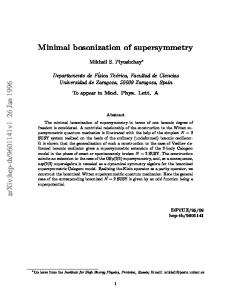
Let us briefly consider the action of the renormalization group (RG) on fermions. The low-energy limit is defined around the Fermi surface. The RG action consists in progressively tracing over degrees of freedom far from the Fermi surface, towards the Fermi surface. In one dimension, this process may be understood better by considering Fig. 1 below. After an RG step wherein the degrees of freedom located in the momentum shell [Λ − dΛ, Λ] have been traced over, one may choose to perform an infinitesimal momentum scale transformation k → (1 + dΛ/Λ)k which brings the cutoff back to its initial value Λ before this RG step. This rescaling is necessary if one wants to compare the new coupling constants with the old ones (i.e. if one wants to define a RG trajectory) since we are then comparing theories with identical cutoffs Λ. In a (nearly) Lorentz invariant theory, it is natural to perform this scale transformation both in momentum and energy (or space and time). In the context of one-dimensional electron systems, Lorentz invariance is an emerging symmetry, valid in the low-energy limit, when the linear approximation to the dispersion relation is acceptable. The Fermi velocity v then plays the role of the velocity of light: it is the only characteristic velocity of the system. Interactions may violate Lorentz invariance and cause the appearance of two characteristic velocities vs and vc (spin-charge separation). However, again in the low-energy limit, the system may then separate into disjoint sectors (spin and charge), each benefiting from Lorentz invari1 In
some applications, leading irrelevant parameters are physically important and must be kept.
3
ance, albeit with different “velocities of light”. In the imaginary-time formalism, Lorentz invariance becomes ordinary spatial-rotation invariance. A field theory with rotation, translation and scale invariance is said to have conformal invariance. Fixed point theories, such as the free boson or the free fermion theories (and many interacting theories) are thus conformal field theories. A decent introduction to conformal field theory is beyond the scope of such a short tutorial. The subject is quite vast and has ramifications not only in the field of strongly correlated electrons, but also in the statistical physics of two-dimensional systems, in string theory and in mathematical physics in general. We will simply mention minimal implications of conformal symmetry in bosonization. Of course, departures from fixed points break this symmetry partially, but their effect at weak coupling may be studied in the conformal symmetry framework with profit.
2.2
Conformal transformations
By definition, a conformal transformation is a mapping of space-time unto itself that is locally equivalent to a rotation and a dilation. In two dimensions, and in terms of the complex coordinate z, it can be shown that the only such transformations have the form z→
az + b cz + d
ad − bc = 1
(1)
where the parameters a, b, c, d are complex numbers. In dimension d, the number of independent parameters of such transformations is (d + 1)(d + 2)/2, and d = 2 is no exception. However, the case of two dimensions is very special, because of the possibility of local conformal transformations, which have all the characters of proper conformal transformations, except that they are not oneto-one (they do not map the whole complex plane onto itself). Any analytic mapping z → w on the complex plane is locally conformal, as we known from elementary complex analysis. Indeed, the local line element on the complex plane transforms as � � dw dz (2) dw = dz The modulus of the derivative embodies a local dilation, and its phase a local rotation. This distinctive feature of conformal symmetry in two-dimensional space-time is what allows a complete solution of conformal field theories, even in circumstances that apparently break scale invariance. For instance, the entire complex plane (the space-time used with imaginary time at zero temperature) may be mapped onto a cylinder of circumference L via the complex mapping z = e2πw/L . This allows for the calculation of correlation functions in a system with a macroscopic length scale (a finite size L at zero temperature, or a finite-temperature β = L/v in an infinite system) from the known solution in a scale-invariant situation. Mappings may also be performed from the upper half-plane unto finite, open regions; such mappings are particularly useful when studying boundary or impurity problems. On the formal side, this feature of conformal field theory makes the use of complex coordinates very convenient: In terms of x and imaginary time τ = it, these coordinates may be defined as z = −i(x − vt) = vτ − ix (3) z¯ = i(x + vt) = vτ + ix with the following correspondence of derivatives: � � i 1 ∂z = − ∂t − ∂x 2 v � � i 1 ∂t + ∂x ∂z¯ = − 2 v 4
∂x = −i(∂z − ∂z¯) ∂t = iv(∂z + ∂z¯)
(4)
A local operator O(z, z¯) belonging to a conformal field theory is called primary (more precisely, quasi-primary) if it scales well under a conformal transformation, i.e., if the transformation ¯
O′ (αz, α ¯ z¯) = α−h α ¯−h O(z, z¯)
(5)
¯ are a fundamental property of the is a symmetry of correlation functions. The constants h and h operator O and are called the right- and left-conformal dimensions, respectively. Under a plain ¯ is the ordinary dilation (α = α ¯ ), the operator scales as O′ (αz, α¯ z ) = α−∆ O(z, z¯), where ∆ = h + h scaling dimension of the operator. Under a rotation (or Lorentz transformation), for which α = eiθ and α ¯ = e−iθ , the operator transforms as O′ ( eiθ z, e−iθ z¯) = eisθ O(z, z¯), where s = h − ¯h is called the conformal spin of the operator. The scaling dimension appears directly in the two-point correlation function of the operator, which is fixed by scaling arguments – up to multiplicative constant: hO(z, z¯)O† (0, 0)i =
2.3
1 z 2h
1 z¯2h¯
(6)
Effect of perturbations
Fixed-point physics helps understanding what happens in the vicinity of the fixed point, in a perturbative sense. Consider for instance the perturbed action Z S = S0 + g dtdx O(x, t) (7) where S0 is the fixed-point action and O an operator of scaling dimension ∆. Let us perform an infinitesimal RG step, as described in the first paragraph of this section, with a scale factor λ = 1 + dΛ/Λ acting on wavevectors; the inverse scaling factor acts on the coordinates, and if x and t now represent the new, rescaled coordinates, with the same short-distance cutoff as before the partial trace, then Z ′ S = S0 + g d(λt)d(λx) O(λx, λt) Z = S0 + gλ2−∆ dtdx O(x, t) (8) We assumed that we are sufficiently close to the fixed point so that the effect of the RG trace in the shell dΛ is precisely the scaling of O with exponent ∆. By integrating such infinitesimal scale transformations, we find that the coupling constant g scales as g = g0
�
Λ0 Λ
�∆−2
=
�
ξ0 ξ
�2−∆
(9)
where ξ and ξ0 are correlation lengths at the two cutoffs Λ and Λ0 . Thus, the perturbation is relevant if ∆ < 2, irrelevant if ∆ > 2 and marginal if ∆ = 2. A relevant perturbation is typically the source of a gap in the low-energy spectrum. In a Lorentzinvariant system, a finite correlation length is associated with a mass gap m ∼ 1/ξ0 . Let us suppose that the correlation length is of the order of the lattice spacing (ξ ∼ 1) when the coupling constant g is of order unity. The above scaling relation then relates the mass m to the bare (i.e. ‘microscopic’) coupling constant: 1/(2−∆) m ∼ g0 (10) Given the warning issued in the introduction on the impossibility of knowing the bare parameters of the theory with accuracy, we should add that ‘bare’ may mean here “at a not-so-high energy scale 5
where the coupling g0 is known by other means”. In fact, this scaling formula works surprisingly well even if g0 is taken as the bare coupling (at the natural cutoff Λ0 ), provided g0 is not too large. Conformal field theory techniques may also be used to treat marginal perturbations, in performing the equivalent of one-loop calculations in conventional perturbation theory, with the so-called operator product expansion. This is explained in Appendix A and an example calculation is given (more can be found in Refs [2, 3, 4]). However, perturbations with conformal spin s 6= 0 are more subtle, and typically lead to a change in kF or incommensurabilities.
2.4
The central charge
A conformal field theory is characterized by a number c called the conformal charge. This number is roughly a measure of the number of degrees of freedom of the model considered. By convention, the free boson theory has conformal charge c = 1. So does the free complex fermion. A set of N independent free bosons has central charge c = N . Conformal field theories with conformal charge c < 1 correspond to known critical statistical models, like the Ising model (known since Onsager’s solution to be equivalent to a free Majorana fermion), the Potts model, etc. Models at c = 1 practically all correspond to a free boson or to slight modifications thereof called orbifolds, and have been completely classified [5]. A conformal field theory of integer central charge c = N may have a representation in terms of N free bosons, although such representations are not known in general. Likewise, a conformal field theory of half-integer central charge may have a representation in terms of an integer number of real (i.e. Majorana) fermions.
3 3.1
Interacting electrons in one dimension Continuum fields and densities
Let us consider noninteracting electrons on a lattice and define the corresponding (low-energy) field theory. This poses no problem, since the different momentum scales of this free theory are decoupled. The microscopic Hamiltonian takes the form X HF = ε(k)c† (k)c(k) (11) k
where c(k) is the electron annihilation operator at wavevector k (we ignore spin for the time being). The low-energy theory is defined in terms of creation and annihilation operators in the vicinity of the Fermi points (cf. Fig. 1) as follows: α(k) α(−k) β(k) β(−k)
= = = =
c(kF + k) c(−kF − k) c† (kF − k) c† (−kF + k)
where k is positive. The noninteracting Hamiltonian then takes the form Z � dk v|k| α† (k)α(k) + β † (k)β(k) HF = 2π
(12)
(13)
where v is the Fermi velocity, the only remaining parameter from the microscopic theory. The energy is now defined with respect to the ground state and the momentum integration is carried between −Λ and Λ. The operators α(k) and β(k) respectively annihilate electrons and holes around the right Fermi point (k > 0) and the left Fermi point (k < 0). A momentum cutoff Λ is implied, which corresponds to an energy cutoff vΛ. Note that the continuum limit is in fact a low-energy limit: Energy considerations determine around which wavevector (±kF ) one should expand. In position 6
electrons
vF Λ
EF holes
–kF (L)
0
kF (R)
π
Figure 1: Typical tight-binding dispersion in 1D, illustrating left and right Fermi points and the linear dispersion in the vicinity of those points. space, this procedure amounts to introducing slow fields ψ and ψ¯ such that the annihilation operator at site n is2 c ¯ e−ikF x √x = ψ(x) eikF x + ψ(x) (14) a √ The factor a is there to give the fields the proper delta-function anticommutator, and reflects their (engineering) dimension: {ψ(x), ψ † (x′ )} ¯ {ψ(x), ψ¯† (x′ )} {ψ(x), ψ¯† (x′ )}
= δ(x − x′ ) = δ(x − x′ ) = 0
(15)
Left-right separation The mode expansions of the continuum fields are Z � dk � ikx e α(k) + e−ikx β † (k) ψ(x) = Zk>0 2π � dk � ikx ¯ ψ(x) = e α(k) + e−ikx β † (k) k0 � dk � k¯z ¯ z) = e α(k) + e−k¯z β † (k) (17) ψ(¯ k0 � 1 �¯ dk ¯ z) = √ b(k) e−k¯z + ¯b† (k) ek¯z φ(¯ 2π 2k k>0
φ(z) =
Z
(36)
The variables z and z¯ are defined as in Eq. (3). Note that wavevectors now take only positive values, since we have defined ¯b(k) ≡ b(−k). 11
The dual field It is customary to introduce the so-called dual boson ϑ(x, t), defined by the relation ∂x ϑ = −Π = ¯ this becomes (cf Eq. (4)) − v1 ∂t ϕ. In terms of right and left bosons φ and φ, 1 ∂x ϑ = − ∂t ϕ v ¯ = −i(∂z + ∂z¯)(φ + φ) ¯ = −i(∂z − ∂z¯)(φ − φ) ¯ = ∂x (φ − φ)
(37)
¯ modulo an additive constant which we set to zero. One may then write therefore θ = φ − φ, φ=
1 φ¯ = (ϕ − ϑ) 2
1 (ϕ + ϑ) 2
(38)
if one desires a definition of φ and φ¯ that stands independent from the mode expansion. Since ϑ is expressed nonlocally in terms of Π (i.e., through a spatial integral), the above expression makes it clear that the right and left parts φ and φ¯ are not true local fields relative to ϕ. The basic definition of ϑ in terms of Π implies the equal-time commutation rule [ϕ(x), ϑ(x′ )] = −iθ(x − x′ )
(39)
(please note that θ(x) is the step function [6= ϑ]) which further shows the nonlocal relation between ϕ and ϑ (the commutator is nonzero even at large distances).
4.3
Bose representation of the fermion field
After this introduction of the boson field, let us proceed with a heuristic (and incomplete) derivation of the bosonization formula. The basic idea is the following (we ignore spin for the moment): the electron density ntot. being bilinear in the electron fields, it has Bose statistics. Let us suppose that it is the derivative of a boson field: ntot. ∝ ∂x ϕ. Then Z ∞ 1 dy ntot. (y) ntot. (x) = − ∂x ϕ(x) ϕ(x) = λ (40) λ x where λ is a constant to be determined. Creating a fermion at the position x′ increases ϕ by λ if x < x′ . This has the same effect as the operator " # Z ′ x
exp −iλ
dy Π(y)
(41)
−∞
which acts as a shift operator for ϕ(x) if x < x′ , because of the commutation relation # � " Z x′ i (x < x′ ) dy Π(y) = ϕ(x), 0 (x > x′ ) −∞
(42)
Thus, a creation operator ψ † (x′ ) or ψ¯† (x′ ) may be represented by the above operator, times an operator that commutes with ϕ ( eiαϕ , for instance). This extra factor must be chosen such that ψ † depends on x − vt only, and ψ¯† on x + vt only. The left-right decomposition (35) and Eq. (38) are useful here. Since 1 (43) Π = ∂t ϕ = −∂x ϑ v 12
we have − iλ
Z
x′
dy Π(y) = iλϑ(x′ )
(44)
−∞
from which purely right- and left-moving fields may be obtained by adding or subtracting − 21 iαϕ(x′ ). Thus, a sensible Ansatz for a boson representation of electron creation operators is ¯ ψ¯† (x) = A e−2iλφ(x)
ψ † (x) = A e2iλφ(x)
(45)
where the constants A and λ are to be determined, for instance by imposing the anticommutation relations (15). This will be done below. The one-electron states ψ † |0i, being generated by exponentials of boson creation operators, are coherent states of the boson field φ.4 On the other hand, the elementary Bose excitations (the mesons, in field-theory jargon) are collective density (or spin) fluctuations, i.e., electron-hole excitations.
5
Details of the Bosonization Procedure
5.1
Left and right boson modes
The mode expansions (32) may seem reasonable, but are actually incomplete, for the following reasons: 1. The field being massless, the mode expansion is ill-defined at k = 0, because ω(k = 0) = 0. The mode at k = 0, or zero-mode, has to be treated separately and turns out to be important. The existence of this mode apparently spoils the left-right separation of the field ϕ. 2. In order for bosonization to be rigorously defined, the field ϕ must have an angular character. In other words, the target space of the field must be a circle of radius R (to be kept general for the moment), so that ϕ and ϕ + 2πR are identified. We say that the boson is compactified on a circle. 3. A rigorous proof of bosonization procedure (at the spectrum level) is best obtained on a system of finite size L with periodic boundary conditions. Taking the above remarks into account leads to the following improved mode expansion for the boson field ϕ(x, t): ϕ(x, t) = q +
� π0 vt π ˜0 x X 1 � √ bn e−kz + b†n ekz + ¯bn e−k¯z + ¯b†n ek¯z + + L L 4πn n>0
(46)
Wavevectors are now quantized as k = 2πn/L (n an integer). The creation and annihilation operators have a different normalization from Eq. (32), so as to obey the commutation rules [¯bn , ¯b†m ] = δmn
[bn , b†m ] = δmn
(47)
The zero-mode is treated explicitly as a pair of canonical variables q and π0 obeying the commutation rule [q, π0 ] = i (48) Defining ϕ on a circle of radius R has two consequences: 4 The interactions g and g give the boson Hamiltonian the sine-Gordon form (cf. Sect. 5.6). In that case, 1 3 one-electron states correspond to solitons (kinks) of the sine-Gordon theory.
13
1. The operator q is not single-valued, since it is an angular variable (q and q+2πR are identified). Only exponentials einq/R , where n is an integer, are well defined. Because π0 is conjugate to q, we have the relation n (49) e−inq/R π0 einq/R = π0 + R (the exponential operators shifts the eigenvalues of π0 ). Starting with the π0 = 0 ground state, this means that the spectrum of π0 is restricted to Z/R. 2. Winding configurations are allowed; the constant π ˜0 is precisely defined as π ˜0 = 2πRm, where m is the number of windings of ϕ as x goes from 0 to L. It turns out to be useful to introduce an operator π ˜0 , defined by its eigenvalues 2πRm. This operator commutes with all other operators met so far, but one may define an operator q˜ conjugate to π ˜0 , i.e., such that [˜ q, π ˜0 ] = i. The separation between left- and right-moving parts may then be done in spite of the existence of a zero mode: X 1 P √ φ(z) = Q + (vt − x) + (bn e−kz + b†n ekz ) 2L 4πn n>0 X 1 ¯ P ¯ ¯+ √ (¯bn e−k¯z + ¯b†n ek¯z ) (50) (vt + x) + φ(z) = Q 2L 4πn n>0 where we have defined the right and left zero-modes Q = ¯ = Q
1 (q − q˜) 2 1 (q + q˜) 2
P = π0 − π ˜0
[Q, P ] = i
P¯ = π0 + π ˜0
¯ P¯ ] = i [Q,
(51)
¯ The spectrum of P and Note that the “artificial” operator q˜ drops from the combination ϕ = φ + φ. ¯ P is �n � � �n P = + 2πRm − 2πRm (52) P¯ = R R m and n being integers. Note that this spectrum is not a simple Cartesian product, which means that the left-right decomposition of the boson is not perfect, despite the expansion (50).
5.2
Proof of the bosonization formulas: Vertex operators
Before investigating the constants A and λ of Eq. (45), serious questions must be asked on the precise definition of an exponential operator of the form eiαφ (such operators are called vertex operators, from their usage in string theory). Because φ is a fluctuating field, any power or more complicated function of φ requires a careful definition if it is not to have a divergent average value. The natural prescription is called normal ordering and consists in expressing φ as a mode expansion and putting all annihilation operators to the right of creation operators. Thus, the exponential operator has the following precise definition: # " # " X 1 X 1 † kz −kz iαφ(x−vt) iαQ √ √ exp iα e−iαP (x−vt)/2L (53) bn e bn e :e := e exp iα 4πn 4πn n>0 n>0 where P is considered an annihilation operator since the boson ground state |0i has zero momentum. The notation :A: means that the operator A is normal ordered. Because of normal ordering, vertex operators do not multiply like ordinary exponentials. Instead, one has the relation ′ ′ ′ eiαφ(z) eiβφ(z ) = eiαφ(z)+iβφ(z ) e−αβhφ(z)φ(z )i (54) 14
where hφ(z)φ(z ′ )i is a simple ground state expectation value if the left-hand side is an ordinary product, or a Green function if it is a time-ordered product. This is one of the most important formulas of this review, and it can be easily demonstrated using the Campbell-Baker-Hausdorff (CBH) formula: 1 eA eB = eA+B e 2 [A,B] ([A, B] = const.) (55) Consider for instance a single harmonic oscillator a, and two operators A = αa + α′ a†
B = βa + β ′ a†
(56)
The CBH formula allows for a combination of the normal-ordered exponentials: : eA :: eB : = = =
′ †
′ †
eα a eαa eβ a eβa ′ † ′ † ′ eα a eβ a eαa eβa eαβ : eA+B : eh0|AB|0i
(57)
The last equality also applies if (a, a† ) is replaced, in the same order, by a pair (p, q) of canonically conjugate operators ([q, p] = i). It also applies to a combination of independent oscillators, such ¯ Finally, it applies to a time-ordered product as well as to an ordinary as the boson fields φ or φ. product, as long as h0|AB|0i is also replaced by a time-ordered product. Thus, the identity (54) is proven. It remains to calculate the Green function hφ(z)φ(z ′ )i. This can be done in several ways. For instance, by using the mode expansion (50) and taking the limit L → ∞: hφ(z)φ(0)i
=
−
1 X 1 −2πnz/L i (vt − x) + e 2L 4π n>0 n
z 1 2πz − ln 2L 4π L 1 ln z + const. → − 4π =
−
(L → ∞)
(58)
We will adopt the normalization hφ(z)φ(z ′ )i = −
1 ln(z − z ′ ) 4π
(59)
and drop the constant term, which basically defines an overall length scale. Likewise, one finds ¯ z )φ(¯ ¯ z ′ )i = − 1 ln(¯ hφ(¯ z − z¯′ ) 4π
(60)
Another way of computing the boson Green function is to notice that the nonchiral Green function G(x, τ ) = hϕ(x, τ )ϕ(0, 0)i must obey the two-dimensional Poisson equation ∇2 G = δ(x)δ(vτ )
(61)
in Euclidian space-time. The solution to that equation is readily obtained in polar coordinates, up to an additive constant (the correct normalization is obtained by applying Gauss’ theorem around the origin): 1 1 G(x, vτ ) = − ln(x2 + v 2 τ 2 ) = − ln(z z¯) (62) 4π 4π The result is thus equivalent to what can be inferred from the mode expansion, since ¯ z )φ(0)i ¯ hϕ(x, τ )ϕ(0, 0)i = hφ(z)φ(0)i + hφ(¯ 15
(63)
Formula (54) can thus be rewritten as ′
′
eiαφ(z) eiβφ(z ) = eiαφ(z)+iβφ(z ) (z − z ′ )αβ/4π
(64)
We are now in a position to demonstrate the boson-fermion equivalence at the level of the (anti)commutation relations. In fact, it is simpler to determine the constants A and λ of Eq. (45) by comparing Green functions rather than simply looking at equal time (anti)commutators (this avoids the equal time singularity). The electron propagator is readily calculated from the mode expansion (16):5 Z Z ′ dk dq h0|α(k)β † (q)|0i e−kz+qz hψ(z)ψ † (z ′ )i = k>0 2π q>0 2π Z dk −k(z−z′ ) e = k>0 2π 1 1 = (65) 2π z − z ′
where we have supposed that τ > τ ′ , which garantees the convergence of the integral and follows from the prescribed time-ordered product. Likewise, hψ † (z)ψ(z ′ )i =
1 1 2π z − z ′
(66)
The correct anticommutator may be obtained from the equal time limit: {ψ(x, 0), ψ † (x′ , 0)}
= = =
� lim hψ(ε − ix)ψ † (−ix′ )i + hψ † (ε − ix′ )ψ(−ix)i � � 1 1 1 lim + 2π ε→0 ε − i(x − x′ ) ε − i(x′ − x) 2ε 1 = δ(x − x′ ) lim ε→0 2π (x − x′ )2 + ε2
ε→0
(67)
(ψ or ψ¯ appearing with a single argument are considered functions of z or z¯). One easily checks that the space-time Green function (65) has the expected expression in momentum-frequency space: 1 1 1 −→ 2π z − z ′ ω − v|k|
(68)
To demonstrate Eq. (45) and fix the values of A and λ, one needs to calculate ′
hψ(z)ψ † (z ′ )i = A2 h e−2iλφ(z) e2iλφ(z ) i
(69)
From the relation (64), this is hψ(z)ψ † (z ′ )i =
=
′
2
A2 h e−2iλ(φ(z)−φ(z )) i(z − z ′ )−λ 2
A2 (z − z ′ )−λ
/π
/π
(70)
Note that the normal-ordered expectation value ′
h e−iαφ(z)−iβφ(z ) i
(71)
is nonzero only if α + β = 0. This can be inferred from the action of the zero-mode operator Q:6
5 For
h0| ei(α+β)Q e−i(α+β)P/2L |0i
a calculation in the path-integral formalism, see Ref. [6]. 6 It is also a consequence of the U(1) symmetry ϕ → ϕ + a, where a is a constant.
16
(72)
vanishes if α + β 6= 0, since the exponential of Q acting on |0i yields another eigenstate of P , with eigenvalue α + β, orthogonal to |0i. The condition α + β = 0 is called the neutrality condition.7 By √ comparing Eq. (70) with Eq. (65), we conclude that the constant λ must be π and that A must √ be 1/ 2π. The correct bosonization formula is then ψ(x) ¯ ψ(x)
√
= √1 e−i 4πφ(x) 2π √ ¯ = √1 ei 4πφ(x) 2π
√
= √1 ei 4πφ(x) 2π √ ¯ = √1 e−i 4πφ(x) 2π
ψ † (x) ψ¯† (x)
(73)
¯ Notice also that the choice of additive Notice the change of sign in the exponent between ψ and ψ. constant leading to Eq. (60) influences the value of A only, the end result being the same irrespective of that choice. Remarks: 1. It is also instructive to check the anticommutation relation {ψ(x), ψ(x′ )} = 0
(74)
This is done simply by noting that the Green function hψ(z)ψ(z ′ )i =
1 −i√4πφ(z) −i√4πφ(z′ ) e he i 2π
(75)
vanishes, by the neutrality condition. The anticommutator, obtained in the equal-time limit, also vanishes. 2. The vertex operator eiαφ is a scaling field. Its conformal dimension hα may be retrieved from the exponent of the Green function h eiαφ(z) ( eiαφ(0) )† i =
1 z α2 /4π
(76)
and from the relation (6). The same analysis may be applied to a left-moving vertex operator ¯ eiα¯ φ . Thus, α2 ¯ h(α) = 8π h(α) =0 (77) α ¯2 ¯ h(¯ α) = 0 h(¯ α) = 8π Roughly speaking, the boson field has scaling dimension zero and its powers series may produce operators with nonzero scaling dimension because of the necessary normal ordering.
5.3
Bosonization of the free-electron Hamiltonian
The bosonization formulas (73) are the basis of a fermion-to-boson translation of various operators. However, this translation process is often subtle, since normal ordering of these operators is required. ¯ Normal ordering can be constructed from Take for instance the chiral fermion densities J and J. the mode expansion. But a shorter and more elegant way to achieve it is by point splitting, i.e., by defining � � (78) J(z) = lim ψ † (z + ε)ψ(z) − hψ † (z + ε)ψ(z)i ε→0
7 This
terminology comes from an analogy with the Coulomb gas system of two-dimensional statistical mechanics.
17
where ε has positive time (so as to appear as shown after time ordering). This limit must be taken after applying the bosonization formulas and the relation (54): � √ � √ 1 1 lim ei 4πφ(z+ε) e−i 4πφ(z) − J = 2π ε→0 ε � √ � 1 1 1 = lim ei 4π[φ(z+ε)−φ(z)] − 2π ε→0 ε ε � √ � 1 1 1 lim eiε 4π∂z φ(z) − = 2π ε→0 ε ε 1 √ i (79) = i 4π∂z φ = √ ∂z ϕ 2π π where we have Taylor-expanded the exponential on the last line. We proceed likewise for the leftmoving density, except that the sign is opposite. To summarize: i J = √ ∂z ϕ π
i J¯ = − √ ∂z¯ϕ π
(80)
(note that ∂z φ = ∂z ϕ and ∂z¯φ¯ = ∂z¯ϕ). The density fluctuations J and J¯ are also components of a conserved current from the boson point of view. Indeed, the compactified boson has a U (1) symmetry: the Lagrangian is invariant under the shift ϕ → ϕ+a. By Noether’s theorem, this symmetry implies the existence of a conserved quantity, with a density proportionnal to ∂t ϕ and current proportionnal to v 2 ∂x ϕ. It is customary to define right and left ‘currents’ exactly as in Eq. (80), so that the continuity equation reduces to ∂z J¯+ ∂z¯J = 0. In fact, the critical (i.e., massless) and one-dimensional nature of the theory enhance this U (1) symmetry to a chiral U (1) symmetry, by which the left and right currents are separately conserved: (81) ∂z¯J = 0 ∂z J¯ = 0 The same short-distance expansion as in Eq. (79) may be used to demonstrate explicitly the equivalence of the electron Hamiltonian (19) with the boson Hamiltonian (30), except that a higherorder expansion is necessary. More explicitly, an expression like ψ † ∂x ψ must be evaluated as � (82) ψ † ∂x ψ = −i lim ψ † (z + ε)∂z ψ(z) − hψ † (z + ε)∂z ψ(z)i ε→0
The limit is evaluated by using the following short-distance products (to order ε2 ), derived from the bosonization formulas and the relation (54): ψ(z ′ )ψ † (z) = ψ † (z ′ )ψ(z) = ¯ z ′ )ψ¯† (¯ ψ(¯ z)
=
¯ z) ψ¯† (¯ z ′ )ψ(¯
=
1 ε 1 + i √ ∂z ϕ + i √ ∂z2 ϕ − ε(∂z ϕ)2 2πε π 4π 1 1 ε 2 − i √ ∂z ϕ − i √ ∂z ϕ − ε(∂z ϕ)2 2πε π 4π 1 1 ε¯ 2 − i √ ∂z¯ϕ − i √ ∂z¯ ϕ − ε¯(∂z¯ϕ)2 2π¯ ε π 4π 1 1 ε¯ 2 + i √ ∂z¯ϕ + i √ ∂z¯ ϕ − ε¯(∂z¯ϕ)2 2π¯ ε π 4π
(83)
where ε = z ′ − z and ε¯ = z¯′ − z¯, and the fields on the r.h.s. are considered functions of (z, z¯) only, the (z ′ , z¯′ ) dependence residing in the powers of ε and ε¯ only. The limit (82) may be obtained by differentiating with respect to z or z¯ the above expansions, and proceeding to a straightforward
18
substitution. The Hamiltonian (19) then becomes Z � � HF = −v dx (∂z ϕ)2 + (∂z¯ϕ)2 Z � = πv dx J 2 + J¯2
(84)
which is precisely the boson Hamiltonian (30), after using the relations (4). Thus the equivalence between a free fermion and a free boson is demonstrated at the level of the Hamiltonian. Note that we have not demonstrated this equivalence at the Lagrangian level; this cannot be done with the techniques used here.
5.4
Spectral equivalence of boson and fermion
That the free boson (at a certain radius R) is equivalent to a free fermion requires that the spectra of the two theories be identical. This can be tested by comparing the grand partition functions of the two models. Let us try to do it for left and right excitations separately. Consider the right-moving fermion ψ(x), and the corresponding Hamiltonian and fermion number: X X † HF = vk(α†k αk + βk† βk ) NF = (αk αk − βk† βk ) (85) k>0
k>0
where the operators αk and βk have different normalizations from those of Eq. (13) and obey the anticommutation rules {αk , α†q } = δkq {αk , αq } = 0 (86) (and likewise for βk ). The spectrum of the Hamiltonian is encoded in the grand partition function X ZF = e−β(H−µN ) (87) states
We have defined the theory on a cylinder, so as to have discrete wavenumbers. We shall use antiperiodic boundary conditions, known in string theory as Neveu-Schwarz boundary conditions: ψ(x + L) = −ψ(x)
(88)
The wavenumbers are then half-integer moded: k = 2π(n + 12 )/L, where n is a positive integer (by contrast, periodic boundary conditions, also known as Ramond boundary conditions, lead to integermoded wavenumbers and to the presence of a fermion zero-mode). Each mode being independent, the fermion grand partition function factorizes as ZF =
∞ Y
(1 + q n+1/2 t)(1 + q n+1/2 t−1 )
n=1
q ≡ e−2πvβ/L , t ≡ eβµ
(89)
Let us now turn to the boson. We first have to write down an expression for the Hamiltonian in terms of the modes appearing in (50). A straightforward calculation yields HB =
P2 2π X † + nb bn 4L L n>0 n
(90)
for the right-moving part. Let us then notice that the fermion number NF is proportional to the zero-mode P . More precisely, P (91) NF = √ 4π 19
√ This can be shown from the mode expansion (50) and by the equivalence J = −∂x φ/ π, which implies Z 1 P (92) NF = dx J = − √ (φ(L) − φ(0)) = √ π 4π
Each mode bn being independent, the boson grand partition function is then ) (∞ √ X 2 Y � 1 + q n + q 2n + q 3n + · · · ZB = q P /8π tP/ 4π =
(
n=1 ∞ Y
1 1 − qn n=1
P
)
X
qP
2
√
/8π P/ 4π
t
(93)
P
So far we have not determined the boson radius R, nor the spectrum of P . We now invoke Jacobi’s triple product formula: ∞ Y
(1 − q n )(1 + q n−1/2 t)(1 + q n−1/2 t−1 ) =
n=1
X
2
qn
/2 n
t
(94)
n∈Z
Applied to the fermion partition function, this remarkable identity shows that ) (∞ X 2 Y 1 q n /2 tn ZF = n 1 − q n n=1
(95)
√ In order to have ZF = ZB , we therefore need P to take the values P √= n 4π. This is not quite the spectrum (52). The closest it comes to is obtained at radius R = 1/ 4π, where (52) becomes P =
√ 1 4π(n + m) 2
P¯ =
√ 1 4π(n − m) 2
(96)
In fact, because of the imperfect left-right separation of the boson spectrum (52), the equivalence with a perfectly left-right separated fermion theory is impossible. However, a state-by-state correspondence between the two theories exists if some constraints are imposed on the fermion spectrum. Explicitly: 1. One needs to include both periodic and antiperiodic boundary conditions in the fermion theory: the Hilbert space is then the direct sum of two sectors. 2. The periodic sector must contain a single zero-mode ψ0 (the same for left- and right-moving fermions), such that {ψ0 , ψ0† } = 1. The operator ψ0† does not change the energy of a state, but increases the fermion number by one. This mixes (in a weak way) the left and right-moving spectra. 3. the number of fermions in the antiperiodic sector must be even (odd-number states are thrown out). These constraints will not be demonstrated here; a detailed proof can be found in Refs [6] and [7]. That the simple-minded correspondence between left-moving fermions and left-moving bosons is impossible should not bother us too much. The complications mentioned above basically involve boson or fermion zero-modes and boundary conditions. The nonzero frequency modes are not affected and the fermion-boson correspondence works well for those modes, as reflected in the Jacobi triple product formula √ (94). First and foremost, we should retain from this exercise that the boson radius must be R = 1/ 4π in order for the fermion-boson equivalence to hold.
20
5.5
Case of many fermion species: Klein factors
Suppose now that we have more than one fermion species, labelled by a greek index: ψµ . Bosonization would then require an equal number of boson species φµ and the formulas (73) would still be applicable, except for the fact that they do not provide for the anticommutation of different fermion species. In fact, this problem arises for a single species as well, since the left and right fermions ψ and ψ¯ must anticommute, whereas the fields φ and φ¯ commute.8 A possible solution lies in the introduction of additional anticommuting factors, the so-called Klein factors, in the bosonization formulas: √ √ ψµ (x) = √1 ηµ e−i 4πφµ (x) ψµ† (x) = √1 ηµ ei 4πφµ (x) 2π 2π (97) √ √ ¯ ¯ ψ¯†µ (x) = √1 η¯µ e−i 4πφµ (x) ψ¯µ (x) = √1 η¯µ ei 4πφµ (x) 2π 2π The Klein factors ηµ and η¯µ are Hermitian and obey the Clifford algebra: {ηµ , ην } = {¯ ηµ , η¯ν } = 2δµν
{ηµ , η¯ν } = 0
(98)
Klein factors act on a Hilbert space distinct from the boson Hilbert space generated by the modes of Eq. (50). This Hilbert space expansion must be compensated by some sort of “gauge fixing”: the Hamiltonian must be diagonal in this Klein factor space, as well as required physical observables. Then, one Klein eigenstate is chosen and the rest of the Klein Hilbert space decouples. An alternative to Klein factors, which requires no extra Hilbert space, is to include in the bosonization formula for ψµ the factor # " √ " # X πX exp iπ NF,ν = exp i (99) Pν 2 ν 2π(Ks − 1) (g1 is then said to be marginally relevant) while it flows to g1 = 0 if |g1 ] < 2π(Ks − 1) (g1 is then said to be marginally irrelevant). Thus, we expect a spin gap for g1 infinitesimal and Ks < 1.15 This expectation is fullfilled exactly at the special value Ks = 21 . There, the cosine term has scaling dimension 1 and is precisely what one would obtain from bosonizing the Dirac mass term of Eq. (23), except that the corresponding fermion represents not electrons, but massive spinons. This Ks = 1 theory is called the Luther-Emery model [9] and is a free theory for spinons, even though it is a complicated interacting theory for electrons (and who knows what happens in the charge sector at the same time. . . ). The above analysis can be repeated for the Umklapp term (111), which occurs only at half filling. One simply has to replace g1 by g3 and Ks by Kc . Thus, a charge gap develops if Kc < 1 (i.e. if g2,c is repulsive) or if |g3 ] > 2π(Kc − 1). Again, free massive holons occur at Kc = 12 .
7 7.1
Non-Abelian bosonization Symmetry currents
The bosonization procedure described in Sect. 5 is often called Abelian bosonization, because a single compactified boson ϕ has a U (1) symmetry ϕ → ϕ + a and the group U (1) is Abelian (i.e. commutative). Abelian bosonization may be used to describe the spin sector of a 1D electron gas, but this description is not manifestly spin-rotation invariant. Indeed, the chiral currents associated to the three spin components are easily shown to be Jz
=
Jx
=
Jy
=
1 † i ψ (σ3 )αβ ψβ = √ ∂z ϕs 2 α 2π � �√ 1 † i 8πφs ψα (σ1 )αβ ψβ = η↑ η↓ sin 2 2π �√ � i 1 † ψα (σ2 )αβ ψβ = − η↑ η↓ cos 8πφs 2 2π
(138)
The z component manifestly has a special role in this representation. While the correlations hJ a (x)J a (0)i (a = x, y, z) all decay with the same power law, they do not have the same normalization, a somewhat unsatisfactory feature. Fortunately, there exists a bosonization procedure that is manifestly symmetric under the spin rotation group SU(2), or under any Lie group for that matter. This non-Abelian bosonization expresses a set of fermion fields in terms of a matrix field belonging to a representation of a Lie algebra, instead of one or more simple boson fields. The corresponding boson theory, the Wess-Zumino-Witten (WZW) model, is far less familiar than the ordinary boson. But in all situations where symmetry considerations (including symmetry breaking) are important, non-Abelian bosonization is the method of choice. It is of course unrealistic to give a rigorous and complete introduction to the WZW model and non-Abelian bosonization within this brief tutorial. Ref. [6] may be consulted for an in-depth discussion. Let us first return to Abelian bosonization and insist on the role of the U(1) current, before generalizing to larger symmetry groups. The currents associated with the U(1) symmetry are given in Eq. (80) for a single species of fermions and coincide with the chiral fermion density fluctuations. For the charge U(1) symmetry, it is the total (↑+↓) density fluctuation that matters, and the charge 15 Note that the sign of g is of no consequence: it is the result of a gauge choice through Klein factors. The 1 arbitrariness in the sign of g1 may be traced back to its expression in terms of left and right fermions: changing the sign of either ψ↑ , ψ¯↑ , ψ↓ or ψ¯↓ is of no consequence in the noninteracting case, but changes the sign of g1 and g3 , without affecting those of g2 or g4 .
28
currents are therefore
i Jc = √ ∂z ϕc 2π
i J¯c = − √ ∂z¯ϕc 2π
(139)
In terms of the U (1) group element g = eiϕc , these currents are proportional to g −1 ∂z g and g −1 ∂z¯g. The charge Hamiltonian can then be expressed in terms of these currents, as in Eq. (84): Z � πvc (140) dx Jc2 + J¯c2 H= 2
This is enough to define the theory, provided that (i) the commutation relations of the currents are specified: i (141) [Jc (x), Jc (x′ )] = − δ ′ (x − x′ ) π and (ii) the vertex operators are introduced, with their proper commutations with the currents. Note: The above current commutation relation can be demonstrated in the same way as we have recovered the fermion anticommutation relations (67), from the current-current correlation function hJc (z)Jc (z ′ )i =
1 1 8π 2 (z − z ′ )2
(142)
obtained from Eq. (59) by differentiating w.r.t. z and z ′ . Likewise, non-Abelian bosonization (for SU(2)) may be introduced starting with the various components of the spin currents Ja defined above in terms of two electron fields ψσ , and expressed in terms of a group element g as X ¯ z ) = g −1 (∂z¯g) = 1 J(¯ J¯a σa 2 a
1X Ja σa 2 a
J(z) = (∂z g)g −1 =
(143)
The Hamiltonian of the SU(2) WZW model can be expressed in terms of these SU(2) currents: 3
2πv X H= k + 2 a=1
Z
� � dx :J a (x)J a (x): + : J¯a (x)J¯a (x):
(144)
where the integer k is called the level of the WZW model, and where the currents now obey the following commutation rules [J a (x), J b (x′ )] [J¯a (x), J¯b (x′ )] [J a (x), J¯b (x′ )]
ik δab δ ′ (x − x′ ) + iεabe J e (x)δ(x − x′ ) 2π ik = − δab δ ′ (x − x′ ) + iεabe J¯e (x)δ(x − x′ ) 2π = 0
= −
(145)
Once the currents are Fourier expanded as J a (z) =
1 X a i2πnz/L J e L n n
(146)
The above commutators translate into the following set of commutation rules, known as a Kac-Moody algebra: a [Jm , Jnb ] = a ¯b [J¯m , Jn ] =
1 e iεabe Jm+n + knδab δm+n,0 2 1 e ¯ iεabe Jm+n + knδab δm+n,0 2 29
(147)
States of the WZW model are created by applying the operators Jna (n < 0) on the vacuum |0i and on a finite number of spin states. The formulation of the WZW in terms of currents is not as fundamental as its definition in the Lagrangian formalism, in terms of a field g(x, t) taking its values in SU(2) (or in another Lie group). The model must be such that the currents are chiral, i.e. ∂z J¯ = ∂z¯J = 0, and must have conformal invariance. The needed action is Z Z � k ik d3 x εµνλ tr g −1 ∂ µ g g −1 ∂ ν g g −1 ∂ λ g (148) S[g] = d2 x tr(∂ µ g −1 ∂µ g) − 8π 12π B
where the second term is topological: it is integrated in a three-dimensional manifold B whose boundary is the two-dimensional space-time, but its value depends only on the field configuration on the boundary of B. The level k must be an integer in order for the WZW model to have conformal invariance and chiral currents. Working with the action (148) is somewhat unwieldy and almost never done in practice, once key identities (Ward identities) have been derived, leading, among others, to the commutators (145). Bosonization cannot be done in terms of the currents alone. The group elements g occur in the representation of left-right products of fermions, as specified by the Witten formula[10]: ψα ψ¯†β
=
ψ¯α ψβ†
=
√ 1 gαβ e−i 2πϕc 2π √ 1 † (g )αβ ei 2πϕc 2π
(149)
where the presence of the charge boson ϕc is still necessary in order to represent the charge component of the products. This formula leads to the following representation of the charge and spin densities: i h √ 2πntot. (x) = J + J¯ + e−2ikF x ei 2πϕc trg + H.c. h i √ a 2πStot. (x) = J a + J¯a + e−2ikF x ei 2πϕc tr(gσa ) + H.c. (150)
The WZW model is a conformal field theory, with a set of well-identified primary (or scaling) fields. It is completely soluble, in the sense that the structure of its Hilbert space is completely known and correlation functions obey linear differential equations. The central charge of the level-k SU(2) WZW model is 3k (151) c= k+2 and it contains scaling fields of all spins from s = 0 to s = k/2, with conformal dimensions ¯= h=h
s(s + 1) k+2
(152)
The spin part of the 1D electron gas with one band is described by the simplest of all WZW models: SU(2) at level 1. The matrix field g corresponds to s = 21 and has conformal dimensions ( 14 , 14 ). Its components may be expressed in terms of the spin boson ϕs , if we follow Witten’s formula and the Abelian bosonization formulas: ! √ √ e−i√ 2πϕs e−i√ 2πϑs (153) g= ei 2πϑs ei 2πϕs The equivalence of the k = 1 SU(2) WZW model with the spin boson theory is possible because the k = 1 model has central charge unity. Such a correspondence between a WZW model and simple bosons is possible only if c is an integer. 30
Other WZW models describe more exotic critical systems. The biquadratic spin-1 chain, with Hamiltonian X H= Sn · Sn+1 + β(Sn · Sn+1 )2 (154) n
is critical at β = 1 and β = −1. At β = −1, the low-energy limit is described by the k = 2 SU(2) WZW model, which has central charge c = 23 . This model may be expressed in terms of three Majorana fermions [11, 12]. At β = +1, the low-energy limit is described by the k = 1 SU(3) WZW model. A recent attempt at extending Zhang’s SO(5) theory of antiferromagnetism and d-wave superconductivity to one-dimensional systems is formulated in terms of WZW models [13].
7.2
Application to the perturbed Tomonaga-Luttinger model
The noninteracting part of the Tomonaga-Luttinger Hamiltonian may be expressed as follows in terms of charge and spin currents: � 2πv � 2 � πv � 2 ¯2 Jc + J¯c2 + J +J 2 3
H0 =
(155)
It is the sum of a free charge boson and of a k = 1 SU(2) WZW model. The various interactions bosonized in Sect. 5.6 have the following expressions in terms of currents: H1
H2c H4c H2s H4s H3
= −2vg1 (Jx J¯x + Jy J¯y ) = vg2,c Jc J¯c = 1 vg4,c [J 2 + J¯2 ] c
2
c
= 4vg2,s Jz J¯z � � 2v ¯2 = g4,s J2 + J 3 √ vg3 = cos( 8πϕc ) 2 2π
(156)
This correspondence may be established with the help of Eq. (138). It is then manifest that g4,c and g4,s only renormalize the velocity. Moreover, if g1 = −2g2,s , H1 and H2s combine into a single, rotation-invariant interaction: H1 + H2s = 4vg2,s J · ¯ J
(g1 = −2g2,s )
(157)
The spin sector Let us restrict ourselves to this isotropic case, at half-filling, so that g3 6= 0. As we have seen in Fig. 6, the RG flow will bring g3 to strong coupling if |g3 | > −2g2,c and the charge sector will have a gap. At the same time, the coupling g1 flows along the separatrix of Fig. 6, towards the fixed point g1 = 0, Ks = 1 (a detailed RG analysis, following the method described in Appendix A, shows that the separatrix is precisely determined by the condition of rotation invariance g1 = −2g2,s ). Thus, the low-energy limit of the half-filled perturbed TL model is the k = 1 WZW model, provided |g3 | > −2g2,c and g1 = −2g2,s . The appearance of a gap in the charge sector has another consequence, that of changing the scaling dimensions of some operators. Specifically, let us consider the 2kF component of the spin density, which becomes the staggered magnetization at half-filling: Sa2kF
=
1 ¯† 2 ψ i (σa )ij ψj
+ H.c. √ 1 = − gji (σa )ij ei 2πϕc + H.c. 4π √ 1 = − tr(σa g) ei 2πϕc + H.c. 4π 31
(158)
where we have applied Witten’s√formula (149). The√cosine Umklapp term gives ϕc a nonzero expectation value, such that hcos 4πϕc i = 6 0 and hsin 4πϕc i = 0. Neglecting fluctuations around that expectation value, one may write the staggered magnetization density as Sa2kF = const. (tr(σa g) + H.c.)
(159)
¯ = 1 , although it According to Eq. (152) with s = 12 , this operator has scaling dimension ∆ = h + h 2 had ∆ = 1 initially (before the onset of the charge gap). Essentially, the charge contribution to the √ fluctuations, i.e. the operator e±i 2πϕc , also of scaling dimension ∆ = 21 , is frozen; this makes the operator Sa2kF more relevant. The staggered magnetization correlation is therefore decreasing like 1/r, instead of the 1/r2 decay of uniform correlations: hSa2kF (x, t)Sa2kF (0, 0)i =
|x2
const. − v 2 t2 |1/2
(160)
Other Perturbations One may add various relevant or marginally relevant perturbations to the model (155): 1. An Ising-like anisotropy would contribute a term of the form HIsing = λJz J¯z . This term, a correction to g2,s is marginally relevant if λ > 0: it brings the flow above the separatrix of Fig. 6. On the other hand, it is marginally irrelevant if λ < 0, and brings the system towards an XY fixed point. 2. An explicit dimerization, maybe in the form of a staggered hopping term in the underlying Hubbard model. This perturbation would be proportional to the CDW (i.e. 2kF ) component of the electron density. In terms of the WZW field g, this may be obtained by √ replacing the Pauli matrices of Eq. (158) by the unit matrix. At half-filling, the freezing of cos 4πϕc would leave the single scaling field trg in the perturbation: Hdim. = λtrg This term has scaling dimension ∆ = of order m ∼ λ2/3 .
1 2
(161)
and would lead, according to Eq. (10), to a spin gap
3. A uniform external magnetic field B. This couples to the uniform magnetization density Jz +J¯z , producing a perturbation with nonzero conformal spin. It breaks rotation invariance and is best treated within Abelian bosonization. In terms of the spin boson ϕs , the perturbation is λ∂x ϕs , where λ ∝ B. The spin Hamiltonian is then H=
� 1 � 2 v Πs + (∂x ϕs )2 + λ∂x ϕs 2
(162)
(we have supposed Ks = 1, i.e., rotation invariance in the absence of external field). This perturbation can be eliminated from the Hamiltonian by redefining ϕs → ϕs −
λ x v
(163)
In terms of the original electrons, this is almost equivalent to changing the value of kF (almost, because it should have no effect on the charge sector). Basically, the uniform magnetic field introduces some incommensurablility in the spin part of the system.
32
8 8.1
Other applications of bosonization The spin- 12 Heisenberg chain
The spin- 21 Heisenberg model in one dimension may also be treated by bosonization in the low-energy limit. The microscopic Hamiltonian is X� y x z (164) J(Snx Sn+1 + Sny Sn+1 ) + Jz Snz Sn+1 H= n
This Hamiltonian may be mapped to a spinless fermion problem via the Jordan-Wigner transformation: ! n−1 X 1 + † † Snz = c†n cn − Sn = cn exp iπ cm cm (165) 2 m
where the operators cn and c†m obey standard anticommutation relations. In terms of these operators, the Heisenberg Hamiltonian is � X� J 1 1 − (c†n cn+1 + H.c.) + Jz (c†n cn − )(c†n+1 cn+1 − ) H= (166) 2 2 2 n P The fermion number n c†n cn is related to the total magnetization M , in such a way that half-filling corresponds to M = 0, the appropriate condition in the absence of external magnetic field. The continuum limit may then be taken and the bosonization procedure applied. The spinless fermion is then endowed with interactions proportional to Jz . Two of these interaction terms are of the g2 and g4 type and renormalize the boson field ϕ and the velocity v. From comparing with known exact exponents, one derives the following relation between the radius R of the boson and the bare interaction strength Jz : � � ��1/2 1 Jz 1 1 − cos−1 (167) R= √ π J 2π Various correlation functions may be calculated, once the correspondence between spin components and the boson field is known [2]:
For instance,
S z (x)
=
S − (x)
=
1 ∂x ϕ + (−1)x cst. eiϕ/R 2πR n
e−2πiRϑ + (−1)x cst. ei[ϕ/R−2πRϑ] + ei[−ϕ/R−2πRϑ]
hS z (x, t)S z (0, 0)i = =
o
1 (h∂z ϕ(x, t)∂z ϕ(0, 0)i + h∂z¯ϕ(x, t)∂z¯ ϕ(0, 0)i) 16π 3 R +cst.(−1)x h eiϕ(x,t)/R eiϕ(0,0)/R i � � 1 1 1 1 + cst.(−1)x 2 + 3 2 2 2 16π R (x − vt) (x + vt) |x + v t2 |1/4πR2
(168)
(169)
Note that the staggered part √ has a nonuniversal exponent, which depends on Jz /J. At the isotropic point Jz = J, R = 1/ 2π and this exponent is 21 , exactly like the non-Abelian bosonization prediction (160).
33
v
B
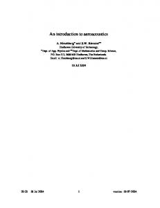
Figure 7: Fluctuation of the edge of a quantum Hall system.
8.2
Edge States in Quantum Hall Systems
The two-dimensional electron gas (2DEG) in a magnetic field has been the object of intense theoretical investigation since the discovery of the quantum Hall effect (integral and fractional) in the early 1980’s. While the integer Hall effect may be understood (in the bulk) on the basis of weakly correlated electrons, the fractional quantum Hall effect is a strongly correlated problem. Quantum Hall plateaus correspond to gapped states, but electric conduction nevertheless occurs through electrons at the edge of the 2D gas, the so-called edge states. One must imagine a 2DEG immersed in a magnetic field B and further confined to a finite area by an in-plane electic field E (in, say, a radial configuration). The field causes a persistent current along the edge of the gas: j = σxy ˆ z∧E
(170)
where σxy is the Hall conductance, equal to νe2 , where ν is the filling fraction. The edge electrons drift in one direction at the velocity v = cE/B. We will adopt a hydrodynamic description of the edge, following Ref. [14]. Let x is the coordinate along the edge and h(x) the transverse displacement of the edge with respect to the ground state shape of the gas (cf. Fig. 7). If n = ν/2πℓ2B is the electron density (ℓB is the magnetic length), then the linear electron density in an edge excitation is J(x) = nh(x). The energy of the excitation is the electrostatic energy associated with the edge deformation: Z Z 1 2 H = dx e hJE = πνv dx J 2 (171) 2 The field J being from the start treated as a collective mode, bosonization is natural. The main difference with the 1D electron gas is that only one half (left of right) of the boson is necessary, since the edge excitations only propagate clockwise or counterclockwise, depending on the field direction. We therefore assert i 1 (172) J = √ ∂x φ = − √ ∂z φ π π and the Hamiltonian density for edge excitations is H = −vν(∂z φ)2
(173)
The filling fraction ν plays the role of a field renormalization K = 1/ν. The edge electron must be represented by a field ψ(x) such that [J(x), ψ(x′ )] = −δ(x − x′ )ψ(x) 34
(174)
From the short-distance product of J with e−iαφ , one finds that the correct representation for ψ is √ 1 ψ(x) = √ ei 4πφ/ν 2π
(175)
From this we derive the one-electron Green function G(x, t) =
1 1 2π (x − vt)1/ν
(176)
Note that this coincides with a free-electron propagator in the case ν = 1 only, i.e., when the first Landau level is exactly filled. Even in the integer effect, the edge system is a Luttinger liquid if m = 1/ν > 1, albeit a chiral Luttinger liquid. In momentum space, the Green function (176) is G(k, ω) ∝
(ω + vk)m−1 ω − vk
(177)
and the momentum-integrated density of states near the Fermi level is N (ω) ∝ |ω|m−1
8.3
(178)
And more. . .
This short tutorial has concentrated on basic Luttinger liquid physics. Time and space are lacking to introduce the many physical systems that have been treated with bosonization. Here we will just indicate a few useful references. The bosonization formalism may also be used to treat disorder. The problem of an isolated impurity in a Luttinger liquid is treated in Refs. [3] and [15], following Kane & Fisher’s original work [16]. The more complicated problem of Anderson localization, resulting from the coherent scattering off many impurities, is also described summarily in Ref. [15]. Formally related to impurity scattering is the question of electron-phonon interaction in a Luttinger liquid, a review of which may be found in Ref. [3]. The Kondo problem, or the strong interaction of magnetic impurities with conduction electrons, has also been treated using bosonization, and a strong dose of conformal field theory, by Affleck and Ludwig. Ref. [17] is a comprehensive review of the progress accomplished with the help of conformal methods. Most interesting in this application is the three-dimensional nature of the initial problem, before it is mapped to a one dimension. Spin chains of spin s > 21 can be constructed from 2s fermion species with a Hund-type coupling. This is the approach followed in Ref. [18], also reviewed in Ref. [2]. The spin-1 chain has been treated as a perturbed k = 2 SU(2) WZW model in Ref. [12]. Coupled spin chains, or spin ladders, have been studied in Abelian bosonization and are reviewed in Ref. [15]. A non-Abelian bosonization study of two coupled spin chains is performed in Ref. [4]. Doped spin ladders are coupled Luttinger liquids. Bosonization studies may be found in Refs. [19] and [20]. Ref. [13] looks at this problem from the perspective of SO(5) symmetry. The latter two references treat the question of d-wave fluctuations in a doped ladder. The reader is referred to Ref. [15, 3] for additional references (we apologize for our poor bibliography). More applications of bosonization to condensed matter can be found in Ref. [3]. Other important review articles on the subject include Refs. [15] and [2]. A historical perspective is given in the collection of preprints [1].
9
Conclusion
Let us conclude by highlighting the principal merits and limitations of bosonization: 35
1. Bosonization is a nonperturbative method. The Tomonaga-Luttinger (TL) model, a continuum theory of interacting fermions, can be translated into a theory of noninteracting bosons and solved exactly. 2. Bosonization is a method for translating a fermionic theory into a bosonic theory, and eventually retranslating part of the latter into a new fermionic language (cf. the Luther-Emery model or the use of Majorana fermions). This translation process is exact in the continuum limit, but does not warrant an exact solution of the model, except in a few exceptional cases (e.g. the TL model). For the rest, one must rely on renormalization-group analyses, which generally complement bosonization. 3. The bosonized theory may have decoupled components, like spin and charge, which are not manifest in fermionic language. Thus, spin-charge separation is an exact prediction of bosonization (even beyond the TL model). When one of the components (spin or charge) becomes massive, this favors the emergence of physical operators with new scaling dimensions, like the staggered magnetization of Eq. (159). 4. The contact with microscopic model is not obvious, since an infinite number of irrelevant parameters stand in the way. But bosonization leads to universal or quasi-universal predictions, and one can argue that such predictions are preferable to the exact solution of a particular microscopic Hamiltonian of uncertain relevance. 5. In the rare cases where a microscopic Hamiltonian has an exact solution (e.g. the 1D Hubbard model), the solution is so complex that dynamical quantities cannot be explicitly calculated. Bosonization can then be used as a complementary approach. Exact values of thermodynamic quantities of the microscopic theory may be used to fix the parameters (e.g. vc , vs , Kc , Ks ) of the boson field theory, and the latter may be used to calculate dynamic quantities (e.g. the spectral weight) or asymptotics of correlation functions[21, 22]. 6. The low-energy limit corresponds to a few regions in momentum-space where bosonization has something to say: the vicinity of wavevectors that are small multiples of kF . 7. Finally, bosonization is limited to one-dimensional systems, despite attempts at generalizing it to higher dimensions [23, 24].
Acknowledgments The author expresses his gratitude to the Centre de Recherches Math´ematiques for making this workshop possible, and to the organizers for inviting him. Support from NSERC (Canada) and FCAR (Qu´ebec) is gratefully acknowledged.
A
RG flow and Operator Product Expansion
In this appendix we show how to derive the approximate RG trajectory around a fixed-point from the Operator Product Expansion (OPE) of the marginal perturbations involved. Consider a fixed-point action S0 describing a conformal field theory, and a set of perturbations with coupling constants gi : X Z gi dxdτ Oi (x, τ ) (179) S[Φ] = S0 [Φ] + i
Here Φ denotes a field or a collection of fields that defines the theory, in the sense of the action and of the path integral measure. The local operators Oi are in principle functions of Φ. The RG 36
procedure may be performed in momentum space or in direct space. It is more convenient here to used the direct space approach and to divide space-time into tiles of side L. A space-time point may then be parametrized as x= X+y (180) where x is a space-time point, X is the space-time coordinate of a tile and y a coordinate within a tile. The RG step is performed by tracing over degrees of freedom labeled by y, leaving us with ˜ “block-spin” degrees of freedom Φ(X). This is done approximately be expanding the perturbations to second order in the partition function, in order to construct an effective action for the “block spin” variables: Z X Z X 1 ˜ ˜ ≈ e−S0 [Φ] 1 − gi dxhOi (x)i> + exp −Seff. [Φ] gi gj dxdx′ hOi (x)Oj (x′ )i> + · · · 2 i
i,j
(181) where the expectations values are taken over the fast modes, i.e., the modes that vary within a tile, in the fixed-point theory. Notice that the fixed-point action S0 is the same for Φ as for the block-spin ˜ precisely because S0 represents a fixed point. field Φ, Consider first the integral Z XZ dyhOi (X + y)i> (182) dxhOi (x)i> = X
tile
¯ i ) are the The integration over the tile of side L may be inferred from dimensional analysis: if (hi , h ¯ conformal dimensions of the operator Oi and ∆i = hi + hi is the corresponding scaling dimension,16 then this integral must be L2−∆i (there is no other quantity with the correct scaling dimension, since the correlation length of the fixed point theory is infinite), times some effective X dependence, so that the first term of Eq. (181) may be written as XX − (183) L2−∆i Oi (X) i
X
where the field Oi (X) denotes this X dependence. The second term of Eq. (181) may be treated in the same way, once the product of operators has been reduced to a sum of single operators by the OPE: Oi (x)Oj (x′ ) =
X
k Cij Ok (x′ )
k
1 |x − x′ |∆i +∆j −∆k
(184)
It is assumed here that the set of operators Oi forms a “closed algebra” under this short-distance expansion. Only the most divergent terms really matter. Let us substitute this OPE in the second term of Eq. (181) and evaluate the integrated expectation value like we did for the first term: we find L2−∆k , times O(X), times the integral over the relative coordinate x − x′ , which scales like L2−∆i −∆j +∆k , or like ln L if 2 = ∆i + ∆j − ∆k . The effective action, after this RG step, is thus given by ( X Z ˜ −S [ Φ] ˜ ≈ e 0 exp −Seff. [Φ] 1− gk dX L2−∆k Ok (X) k
1 XX k gi gj Cij + 2 i,j k
�
L2−∆i −∆j +∆k ln L
�
L
2−∆k
Z
dX Ok (X) + · · ·
)
(185)
16 For simplicity, we will deal with operators of zero conformal spin only, i.e., we suppose that h = h ¯ i . Operators i with nonzero conformal spin naively do not contribute: they have zero expectation value.
37
(a sum over tiles is equivalent to an integral over X, since L is the new ‘lattice spacing’). After reinstalling the perturbations in the exponential, one may define a renormalized coupling gk′ as � 2−∆ −∆ +∆ � i j k 1X k L ′ 2−∆k gk = gk L − L2−∆k (186) Cij gi gj ln L 2 i,j This RG step transformation must be made infinitesimal in order to be translated into an RG flow equation. To this end, we set L very close to unity, in units of lattice spacing, a somewhat formal procedure. In the case of a nonmarginal interaction (∆k 6= 2) the first term dominates in a perturbative sense and, after setting L = eℓ with ℓ small, we find gk′ ≈ gk [1 + (2 − ∆k )ℓ]
→
dgk = (2 − ∆k )gk dℓ
(187)
as expected. A more interesting case is that of a set of marginal interactions (∆k = 2), where gk′ = gk −
1X k C gi gj ln L → 2 i,j ij
dgk 1X k C gi gj =− dℓ 2 i,j ij
(188)
Let us apply this last equation to the spin sector of the 1D electron gas subjected to the interactions g1 and g2 , in order to recover the flow equations (137). Let us first note that, when expanded to first order in g2,s from Eq. (116), those flow equations become dg1 2 = g1 g2 dℓ π
dg2 1 2 = g dℓ 2π 1
(189)
(we dropped the ‘s’ index from now on: it is understood that we deal with the spin sector). The corresponding operators are O1 =
√ 1 cos( 8πϕ) 2π 2
O2 =
2 ¯ ∂ϕ∂ϕ π
(190)
The corresponding OPEs are obtained by applying Wick’s theorem. Their most singular terms are � � 1 1 1 1 1 2 2 ¯ O1 (z, z¯)O1 (w, w) ¯ ∼ − 3 (∂ϕ) + (∂ϕ) 16π 4 (z − w)2 (¯ z − w) ¯ 2 2π (z − w)2 (¯ z − w) ¯ 2 1 1 ¯ ∂ϕ∂ϕ − 3 π (z − w)(¯ z − w) ¯ � � 1 1 1 1 1 2 ¯ 2+ O2 (z, z¯)O2 (w, w) ¯ ∼ − ( ∂ϕ) (∂ϕ) 4π 4 (z − w)2 (¯ z − w) ¯ 2 π 3 (z − w)2 (¯ z − w) ¯ 2 √ 1 1 (191) O2 (z, z¯)O1 (w, w) ¯ ∼ − 4 cos( 8πϕ) 2π (z − w)(¯ z − w) ¯ This last OPE is derived from the relation ¯ ∂ϕ(z) eiαϕ(w,w) ∼−
iα 1 ¯ eiαϕ(w,w) 4π z − w
(192)
which is obtained by applying Wick’s theorem to the series expansion of eiαϕ (see, e.g., Ref. [6]). We may rewrite these OPEs as O1 (z, z¯)O1 (w, w) ¯ ∼ O2 (z, z¯)O2 (w, w) ¯ ∼ O2 (z, z¯)O1 (w, w) ¯ ∼
1 1 O2 (w, w) ¯ + conf. spin 2π 2 (z − w)(¯ z − w) ¯ const. + conf. spin 1 2 O1 (w, w) ¯ − 2 π (z − w)(¯ z − w) ¯ const. −
38
(193)
where ‘conf. spin’ denotes terms with conformal spin, which do not affect the beta functions as calculated above. From Eq. (188), we may then write the flow equations : dg1 1 = 2 g1 g2 dℓ π
dg2 1 2 g = dℓ 4π 2 1
(194)
These differ from Eq. (189) only by a rescaling of the flow variable ℓ by 2π, caused by our crude treatment of kinematic integrals. A corrected version of Eq. (188) would then be X dgk k Cij gi gj = −π dℓ i,j
(195)
References [1] in Bosonization, edited by M. Stone (World Scientific, Singapore, 1994), a collection of reprints. [2] I. Affleck, in Champs, cordes et Ph´enom`enes critiques; Fields, Strings and Critical Phenomena, edited by E. Br´ezin and J. Zinn-Justin (Elsevier, Amsterdam, 1989), p. 564. [3] A. Gogolin, A. Nersesyan, and A. Tsvelik, Bosonization and Strongly Correlated Systems (Cambridge University Press, Cambridge, 1998). [4] D. Allen and D. S´en´echal, Phys. Rev. B 55, 299 (1997). [5] P. Ginsparg, Nucl. Phys. B 295, 153 (1988). [6] P. D. Francesco, P. Mathieu, and D. S´en´echal, Conformal Field Theory (Springer Verlag, New York, 1997), see also the errata page at www.physique.usherb.ca/~dsenech/cft.htm. [7] P. Ginsparg, in Champs, cordes et Ph´enom`enes critiques; Fields, Strings and Critical Phenomena, edited by E. Br´ezin and J. Zinn-Justin (Elsevier, Amsterdam, 1989). [8] J. Kosterlitz and D. Thouless, J. Phys. C:Solid State Phys. 6, 1181 (1973). [9] A. Luther and V. Emery, Phys. Rev. Lett. 33, 589 (1974). [10] E. Witten, Commun. Math. Phys. 92, 455 (1984). [11] A. Zamolodchikov and V. Fateev, Sov. J. Nucl. Phys. 43, 657 (1986). [12] A. Tsvelik, Phys. Rev. B 42, 10499 (1990). [13] D. Shelton and D. S´en´echal, Phys. Rev. B 58, 6818 (1998). [14] X.-G. Wen, Int. J. Mod. Phys. B 6, 1711 (1992). [15] H. Schulz, G. Cuniberti, and P. Pieri, in Fermi liquids and Luttinger liquids, lecture notes of the Chia Laguna (Italy) summer school, september 1997. cond-mat/9807366. [16] C. Kane and M. Fisher, Phys. Rev. B 46, 1220 (1992). [17] I. Affleck, Acta Phys. Polon. B 26, 1869 (1995), cond-mat/9512099. [18] I. Affleck and F. Haldane, Phys. Rev. B 36, 5291 (1987). [19] M. Fabrizio, Phys. Rev. B 48, 15838 (1993). [20] H. Schulz, Phys. Rev. B 53, R2959 (1996). 39
[21] H. Schulz, Phys. Rev. Lett. 64, 2831 (1990). [22] N. Kawakami and S.-K. Yang, Prog. Theor. Phys. (suppl.) 107, 59 (1992). [23] F. Haldane, in Proceedings of the International School of Physics “Enrico Fermi”, edited by R. Broglia and J. Schrieffer (North Holland, Amsterdam, 1994). [24] H.-J. Kwon, A. Houghton, and B. Marston, Phys. Rev. B 52, 8002 (1995).
40