Nov 4, 2008 - At the time, no open-source software combining a CAD engine, a mesh generator and a ... tools were expensive commercial packages [?], and the freeware or shareware tools were ...... This is done for accounting of a singular ...
An introduction to geometrical modelling and mesh generation with Gmsh Christophe Geuzaine
Jean-Fran¸cois Remacle
November 4, 2008
2
Contents 1 Introduction 1.1 The Design of Gmsh . . . . . . . . . . . . . . . . . . . . . . . 1.1.1 Fast and Light . . . . . . . . . . . . . . . . . . . . . . 1.1.2 User-friendly . . . . . . . . . . . . . . . . . . . . . . . 2 Computational Geometry Toolbox 2.1 Delaunay and Vorono¨ı . . . . . . . . . . . . . . 2.1.1 The Vorono¨ı diagram . . . . . . . . . . . 2.1.2 The Delaunay Triangulation . . . . . . . 2.1.3 Construction of Delaunay Triangulations 2.2 Nearest neighbors . . . . . . . . . . . . . . . . . 2.3 Point location . . . . . . . . . . . . . . . . . . .
. . . . . .
. . . . . .
. . . . . .
. . . . . .
. . . . . .
. . . . . .
. . . . . .
5 6 7 8
. . . . . .
11 11 11 14 21 31 31
3 Solid Models 3.1 Boundary Representation of Solids . . . 3.1.1 Geometrical Description . . . . . 3.2 Discrete Representation of the Geometry 3.2.1 Harmonic maps . . . . . . . . . .
. . . .
. . . .
. . . .
. . . .
. . . .
. . . .
. . . .
. . . .
. . . .
. . . .
. . . .
. . . .
33 33 39 49 49
4 Mesh Generation 4.1 Generalities . . . . . . . . . . . . . . 4.1.1 The Euler-Poincar´e Formula . 4.1.2 Mesh generation procedure . . 4.2 Mesh size field and quality measures 4.2.1 Mesh size field . . . . . . . . . 4.3 One Dimensional Meshing . . . . . . 4.4 Planar Meshing . . . . . . . . . . . . 4.5 Surface Meshing . . . . . . . . . . . .
. . . . . . . .
. . . . . . . .
. . . . . . . .
. . . . . . . .
. . . . . . . .
. . . . . . . .
. . . . . . . .
. . . . . . . .
. . . . . . . .
. . . . . . . .
. . . . . . . .
. . . . . . . .
57 57 58 62 64 64 66 67 67
3
. . . . . . . .
. . . . . . . .
4
CONTENTS 4.6 4.7 4.8 4.9 4.10
Quadrilateral Meshing . . . . . . . . . . Tetrahedral Meshing . . . . . . . . . . . Hexaedral Meshing . . . . . . . . . . . . Mesh Data Structures . . . . . . . . . . Structured and Hybrid Mesh Generation 4.10.1 Hyperbolic mesh generation . . . 4.10.2 Elliptic mesh generation . . . . . 4.10.3 Boundary Layer Meshing . . . . . 4.11 Mesh Adaptation . . . . . . . . . . . . . 4.11.1 Local Mesh Modifications . . . . 4.11.2 Interactions with a solver . . . . . 4.12 High Order Mesh Generation . . . . . .
. . . . . . . . . . . .
. . . . . . . . . . . .
. . . . . . . . . . . .
. . . . . . . . . . . .
. . . . . . . . . . . .
. . . . . . . . . . . .
. . . . . . . . . . . .
. . . . . . . . . . . .
. . . . . . . . . . . .
. . . . . . . . . . . .
. . . . . . . . . . . .
. . . . . . . . . . . .
67 67 67 67 67 67 67 67 67 67 67 67
Chapter 1 Introduction When we started the Gmsh project in the summer of 1996, our goal was to develop a fast, light and user-friendly software to easily create geometries and meshes that could be used in our three-dimensional finite element solvers [?], and then visualize and export the computational results with maximum flexibility. At the time, no open-source software combining a CAD engine, a mesh generator and a post-processor was available: the existing integrated tools were expensive commercial packages [?], and the freeware or shareware tools were limited to either CAD [?], two-dimensional mesh generation [?], three-dimensional mesh generation [?, ?, ?], or post-processing [?]. The need for a free integrated solution was conspicuous, and several projects similar in spirit to Gmsh were also born around the same time—some of them still actively developed today [?, ?]. Gmsh however was unique in its design: it consisted of a very small kernel with four modules (geometry, mesh, solver and post-processing), not tied to any particular computational solver, and designed from the start to be driven both using a user-friendly graphical interface (GUI) and its own scripting language. The first public release of Gmsh occurred in 1998. This version was Unix-only, distributed over the internet in binary form, with the graphics layer based on OpenGL [?] and the user interface written in Motif [?]. After several updates and a short-lived Windows-only fork in 2000, the whole user interface was rewritten using FLTK [?] in early 2001, and the code, still in binary-only form, was released for Windows and a variety of Unix operating systems. In 2003 the full source code was released under the GNU General Public License [?], and it was modified to provide native support for all major operating systems: Windows, MacOS and all Unix/X11 variants. In the 5
6
CHAPTER 1. INTRODUCTION
summer of 2006 Gmsh underwent a major rewrite, which led to the release of version 2 of the software in February 2007. About 50% of the code in version 2 is new: an abstract geometrical and post-processing layer has been introduced, the mesh data structures and algorithms have been rewritten from scratch, and the graphics layer has also been completely overhauled. Today Gmsh enjoys a thriving community of several hundred users and developers worldwide. It is driven by the need of researchers and engineers in academia and industry alike for a small, open-source pre- and post-processing solution for grid-based numerical methods. The aim of this paper is not to be a user’s guide or a reference manual—see [?] instead. Rather, it is to present the philosophy and the original features of Gmsh which make it stand out from its free and commercial alternatives. The paper is structured as follows. In Section 1.1 we outline the overall philosophy and design goals of Gmsh, as well as the main technical choices that were made in order to achieve these goals. Sections ??, ??, ?? and ?? then respectively describe the geometry, mesh, solver and post-processing modules. The paper is concluded in Section ?? with perspectives for future developments.
1.1
The Design of Gmsh
Gmsh is built around four modules: geometry, mesh, solver and post-processing. Each module can be controlled either interactively using the GUI or using the scripting language. The design of all four modules relies on a simple philosophy—be fast, light and user-friendly. Fast: on a standard personal computer at any given point in time Gmsh should launch instantaneously, be able to generate a “larger than average” mesh (compared to the standards of the finite element community; say, one million tetrahedra in 2008) in less than a minute, and be able to visualize such a mesh together with associated post-processing datasets at interactive speeds. Light: the memory footprint of the application should be minimal and the source code should be small enough so that a single developer can understand it. Installing or running the software should not depend on any non-widely available third-party software package.
1.1. THE DESIGN OF GMSH
7
User-friendly: the graphical user interface should be designed in such a way that a new user can create simple meshes in a matter of minutes. In addition, the code should be robust, portable, scriptable, extensible and thoroughly documented—all features contributing to a user-friendly experience. In the following sections we describe the technical choices that we made to achieve these sometimes conflicting design objectives. Although major parts of the code have been rewritten over the years, the overall initial architecture and design from 1996 have always stayed the same.
1.1.1
Fast and Light
In order to be fast and light in the sense just described above, Gmsh is entirely written in standard C++ [?]—both the kernel and the user interface. The kernel uses BLAS [?] (through the GSL, the GNU Scientific Library [?]) for most of the basic linear algebra. To keep them easy to understand the algorithms have not been overly optimized for speed or memory usage, yet Gmsh currently generates about a million tetrahedra per minute and per 150 Mb of RAM on a standard personal computer, which makes it powerful enough for many academic and engineering applications. The graphical interface is built using FLTK [?] and OpenGL [?]. Using FLTK instead of a larger or more complex widget toolkit, like for example Java, TCL/TK, GTK or QT, allows to link Gmsh statically with the toolkit. This tremendously reduces the launch time, memory footprint and installation complexity (installing Gmsh requires copying a single executable file), as well as the build time—a statically linked, ready to use executable is produced in a few minutes on a standard personal computer. Analogously, directly using OpenGL instead of a more complex graphics library like Inventor [?] or VTK [?] makes Gmsh lightweight, without sacrificing rendering performance (Gmsh makes extensive use of OpenGL vertex arrays). The design of the solver and scripting interfaces follows the same strategy: the solver interface is written using standard Unix and TCP/IP sockets instead of, e.g., Corba [?], and the scripting interface is built using Lex/Flex and Yacc/Bison [?] instead of using an external scripting language like, e.g., Python.
8
1.1.2
CHAPTER 1. INTRODUCTION
User-friendly
Although Gmsh can be built as a library (which can then be linked with other software tools), it is usually distributed as a stand-alone software, ready to be used by end users. This stand-alone version can be run either interactively using the graphical user interface or in a non-interactive mode—either from the command line or via the scripting language. Achieving “user-friendliness” has been an important driving factor behind key technical choices. We detail some of these choices hereafter, focusing on the list of desirable features given at the beginning of the section. Robustness and Portability To achieve robustness, i.e., working for the largest possible range of input data and being as tolerant as possible to erroneous user input, we use robust geometrical predicates [?] in critical portions of the algorithms, and strive to provide useful error messages when an unmanageable exception is triggered. In order to easily produce a native version of the code on all major operating systems, Gmsh is written entirely in standard C++, and uses portable toolkits for its GUI (FLTK) and graphics rendering (OpenGL). Open-sourcing Gmsh under the GNU General Public License [?] also helped portability, as the code was made part of several official Linux distributions (most notably Debian [?]), and thus benefited from their extensive automated testing infrastructure. Either with the graphical user interface or in batch mode, the same version of Gmsh now runs on most computers, from laptops to workstations and large HPC clusters. Scriptability Gmsh is scriptable so that all input data can be parametrized, and so that Gmsh can be easily inserted as a component inside a larger computational chain. As mentioned above, scripting is implemented in Gmsh using Lex and Yacc. The tight integration with the resulting language means that full access to internal capabilities is provided, including bidirectional access to more than 500 internal options fine-tuning the behaviour of the four modules. The scripting language allows for example to fully parametrize all geometrical entities, to interface external solvers without modifying the source code, or to automate all post-processing operations, e.g., to create complex animations or perform off-screen rendering [?].
1.1. THE DESIGN OF GMSH
9
Extensibility We tried to ease the modification and addition of features by users and developers. Such extensibility takes different forms for each of the four modules: Geometry: the abstract, object-oriented geometry layer permits to write all the algorithms independently of the underlying CAD representation. At the source code level Gmsh is thus easily extensible by adding support for additional CAD engines. Currently two engines are interfaced: the native Gmsh CAD engine and OpenCascade [?]. Adding support for other engines like, e.g., Parasolid [?], can be done simply by deriving four abstract classes—see Section ??. At the scripting level users can then transparently mix and match geometrical parts represented internally by different CAD engines. For example, it is possible to extend an OpenCascade model of an airplane with a terrain model defined in the scripting language. Mesh: using the abstract geometrical interface it is also possible to interface additional meshing kernels. Currently, in addition to its own meshing algorithms (see Section ??), Gmsh is interfaced with Netgen [?] and Tetgen [?]. Solver: a socket-based communication interface allows to interface Gmsh with various solvers without changing the source code; tailored graphical user interfaces can also easily be added when more fine-grained interactions are needed. Post-processing: the post-processor can be extended with user-defined operations through dynamically loadable plug-ins. These plug-ins act on post-processing datasets (called views) in one of two ways: either destructively changing the contents of a view, or creating one or more views based on the current view. All source code-level extensions can be enabled or disabled at compile time thanks to an autoconf-based build mechanism [?], which selects which parts of the code to include/exclude. Documentation and Open File Formats Documentation is provided both in the source code and in the form of a reference manual, including several hands-on tutorial examples and a com-
10
CHAPTER 1. INTRODUCTION
prehensive web site with several mailing lists and a wiki. Another important feature contributing to user-friendliness is the availability of standard input and output file formats. Gmsh uses open or de facto standard formats whenever possible, from standard bitmap graphics formats (JPEG, GIF, PNG) and vector formats [?] (SVG, PostScript, PDF) to mesh formats (Ideas UNV, Nastran BDF). Combined with the open-source release of the code this greatly facilitates the integration of Gmsh with other computational tools.
Chapter 2 Computational Geometry Toolbox 2.1 2.1.1
Delaunay and Vorono¨ı The Vorono¨ı diagram
Let p1 and p2 be two points of R2 . The mediator M(p1 , p2 ) is the locus of all the points which are equidistant to p1 and p2 : M(p1 , p2 ) = {p ∈ R2 , d(p, p1 ) = d(p, p2 )} where d(., .) is the euclidian distance between two points of R2 , i.e. d2 (p1 , p2 ) = (p2 − p1 ) · (p2 − p1 ).
(2.1)
The equation of the mediator can be found out using this definition (p1 − p) · (p1 − p) = (p2 − p) · (p2 − p) or
1 (p1 − p2 ) · p − 2 (p1 + p2 ) = 0 | {z } pm
This shows that the mediator is the orthogonal bissector of the straight edge linking the two points. The mediator separates the plane into two regions. 11
12
CHAPTER 2. COMPUTATIONAL GEOMETRY TOOLBOX p2
pm
p1
p
M
Figure 2.1: The mediator.
The first region contains all the points that are closer to p1 , the second one contains the ones that are closer to p2 . Any point of R2 /M can be associated to one of those two points. Let us consider a set of N points S = {p1 , . . . , pN }. More specifically, we assume that the points are in general position, by which we mean no four points are cocircular. The Vorono¨ı cell C(pi ) associated to point pi is the locus of points of R2 that are closer to pi than any other point pj , j = 1, . . . , N , i 6= j. The Vorono¨ı cell is constructed as follow. Consider all mediators M(pi , pj ). Each of those mediators define a half plane. The Vorono¨ı diagram is the part of the space that is always closer to pi , i.e. that always associate pi to the point p, for all possible mediators.(see Figure 2.2). The set of all Vorono¨ı cells is called the Vorono¨ı diagram of S (see Figure 2.2). Let us present some remarkable properties of the Vorono¨ı diagram. Property 2.1.1 Vorono¨ı cells are convex polytopes. By definition, each Voronoi region C(pi ) is the intersection of open half planes containing vertex pi . Therefore, C(pi ) is open and convex. Different Vorono¨ı regions are disjoint. Vorono¨ı cells are polygons in 2D, polyhedra in 3D and d-polytopes in dD. Vorono¨ı cells are either closed or open. They can only be open for points that are located on the convex hull of the 2D domain. A point pi of S lies on the convex hull of S if and only if its Vorono¨ı cell C(pi ) is unbounded.
2.1. DELAUNAY AND VORONO¨I
13
pj vI pk pi C(pi )
Figure 2.2: The Vorono¨ı diagram. The Vorono¨ı cell C(pi ) relative to vertex pi is coloured.
14
CHAPTER 2. COMPUTATIONAL GEOMETRY TOOLBOX
Figure 2.3: Two triangulations of S, both containing nt = 13 triangles.
Property 2.1.2 Vorono¨ı points vI are always located at intersection of 3 mediators. Property 2.1.2 is only true if there exist no quadruplets of points in S that are cocircular. If such a set exists, it may happen that a vertex of the Vorono¨ı is at the the intersection of more than 3 mediators. Consider the example of Figure 2.2 where vi is at the intersecion of C(pi ), C(pj ) and C(pk ). Vorono¨ı point vI is loacted at the center of the unique circle passing through pi , pj and pk .
2.1.2
The Delaunay Triangulation
We first define what is a triangulation of S: it is a planar subdivision whose bounded faces are triangles and whose vertices are the points pi of S. Note that all triangulations do not cover the same subset of R2 . In what follows, we consider that the domain to triangulate is the convex hull of S. Even with the same domain to cover, several triangulations are possible (see Figure 2.3). Yet, every triangulation has the same number of triangles and edges! Property 2.1.3 Let S be a set of N points in the plane, not all collinear, and let Nh denote the number of points in S that lie on the convex hull of
2.1. DELAUNAY AND VORONO¨I
15
S. Then any triangulation of S has nt (N, Nh ) = 2N − 2 − Nh triangles and ne (N, Nh ) = 3N − 3 − Nh edges. Proof Consider first that all the points in S are in the convex hull: N = Nh . A triangulation consist simply in triangles tI (p1 , pi , pi+1 ), i = 2, . . . , N − 1. The number of triangle is therefore nt = N − 2 wich is consistent with the formula. The number of edges in the triangulation is calculated as follows: Nh = N edges on the convex hull and N − 3 internal edges wich gives ne = N + N − 3 = 2N − 3 which is again consistent with the proposition. The rest of the proof works using a recurrence argument. Assume that formulas are true for N . Let us now consider one new vertex pN +1 that lies inside the convex hull. This new vertex lies inside one of the existing triangles, say tI (pi , pj , pk ). We remove tI and replace it by three new triangles tJ (pi , pj , pN +1 ), tJ (pj , pk , pN +1 ), tJ (pk , pi , pN +1 ). We have therefore nt (Nh , Nh ) = Nh − 2 and nt (N + 1, Nh ) = nt (N, Nh ) + 2 which gives nt (N, Nh ) = Nh − 2 + 2(N − Nh ) = 2N − 2 − Nh . Similarly, three new edges have been added in the process. Then, ne (Nh , Nh ) = 2Nh − 3 and ne (N +1, Nh ) = ne (N, Nh )+3 which gives ne (N, Nh ) = 2Nh −3+3(N −Nh ) = 3N − 3 − Nh . Consider a triangulation T with nt triangles. This triangulation has 3nt internal angles. Consider the vector of angles A(T ) = (α1 , . . . , α3nt ) sorted by increasing values. We can define such a vector for any triangulation of the convex hull of the domain. Each of those vectors has the same length and it is therefore possible to compare them, e.g. lexicographically. We say that one given triangulation T is angle-optimal if A(T ) ≤ A(T 0 ), ∀T 0 . According to that criterion, left triangulation of Figure 2.3 is better than the right one. Angle-optimal trianglations have interresting interpolation properties and it is therefore useful to find methods that allow to construct such triangulations. For a given set of points, the (unique) angle-optimal triangulation is the triangulation that has the highest minimal angle. Let us see now how to build such a triangulation. Consider now the edge e(p4 , p6 ) of Figure 2.4. This edge is surrounded by two triangles t1 (p4 , p6 , p1 ) and t2 (p4 , p6 , p2 ) . An edge swap is a local mesh modification operator that consist in changing locally the triangulation by replacing edge e(p4 , p6 ) by e0 (p1 , p2 ). Triangles t1 (p4 , p6 , p1 ) and t2 (p4 , p6 , p2 ) are replaced by t01 (p1 , p2 , p4 ) and t02 (p1 , p2 , p6 ). Figure 2.4 illustrate the edge swap operation.
16
CHAPTER 2. COMPUTATIONAL GEOMETRY TOOLBOX p2
p2 α1 α20
α1
α6 α5 p6
e t2 α4
t02
t1
t1 α2 α3
e0
p4 α60 p6
p1
α30
p4
α50 α3 p1
Figure 2.4: Edge swap.
It is indeed possible to use the edge swap operator in order to build angleoptimal triangulation. In that purpose, we can simply decide to swap edge e if min (α1 , . . . , α6 ) < min (α10 , . . . , α60 ). Such an edge is said invalid. Given a finite set of points, there is a finite number of possible triangulations. When the angle criterion is applied, every edge swap produce a new triangulation that is better than the actual one. Therefore, building the angle-optimal triangulation consist in looping over all the edges of the mesh and swap them until the optimal configuration is attained i.e. when no invalid edges remain in the triangulation. Figure 2.5 illustrate that procedure. Yet, computing angles is a costly operation and it is possible to use a simpler and cheaper rule to verify the validity of an edge. Property 2.1.4 Let C be a circle, l a line intersecting C in points p4 and p6 and p1 , and p2 , p3 and p5 points lying on the same side of l . Suppose that p2 and p3 lie on C, that p5 lies inside C, and that p1 lies outside C. Then (see Fig. 2.6): α1 < α2 = α3 < α5 . Property 2.1.5 [Lawson’s Criterion] Consider an edge e with its two neighboring triangles t1 and t2 . Consider the circumcircle C of triangle t1 and point p that belongs to t2 but not to t1 . Edge e is invalid if p ∈ C.
2.1. DELAUNAY AND VORONO¨I
17
Figure 2.5: Building an angle-optimal triangulation using swaps.
p1
p2
α1
α2
p5 α5
p3 α3
l p4
p6 C Figure 2.6: Theorem of Thal`es
18
CHAPTER 2. COMPUTATIONAL GEOMETRY TOOLBOX p2 C
0
α0 e0 e
p4
α C
p6 p1
Figure 2.7: Lawson’s criterion
Property 2.1.5 has been demonstrated by Sibson in [?]. Consider Figure 2.7. The proof consist in demonstrating that α0 > α if p1 ∈ C. The demonstration make use of property 2.1.4 (Thal`es’s Theorem). Note that, when two neighboring triangles separated by an edge e form a concave quadrilateral, edge e is always valid. Procedure described in Figure 2.5 allow to build angle-optimal triangulations. Yet, it can be shown that such an algorithm is slow in practice. There exists a much faster manner to build angle optimal triangulations of S that is based on the Vorono¨ı diagram. This triangulation DT (S) is called the Delaunay triangulation and its construction works as follows. First recall that each Vorono¨ı cell C(pi ) is associated to one only point pI of S. Consider a Vorono¨ı point vI that at the meeting point of 3 Vorono¨ı cells C(pi ), C(pj ), C(pk ). Beacuse of the Vorono¨ı property, point v is at the circumcenter of triangle tI (pi , pj , pk ). Triangle tI ∈ DT (S) is one of the triangles of the Delaunay triangulation. The resulting figure is a triangulation (see Figure 2.8). Property 2.1.6 Let S be a set of points in the plane. (i) Three points pi , pj and pk ∈ S are vertices of the same triangle tI of the Delaunay triangulation if and only if the circumcircle C(tI ) contains no point of S in its interior.
2.1. DELAUNAY AND VORONO¨I
19
Figure 2.8: The Vorono¨ı diagram and its associated Delaunay triangulation
20
CHAPTER 2. COMPUTATIONAL GEOMETRY TOOLBOX p2
C(t)
v0 v
p3 lc
t p1
a
b
la
lb
c
Figure 2.9: Illustration of why property (i) of 2.1.6 is true.
(ii) Two points pi and pj ∈ S form an edge eI of the Delaunay triangulation if and only if there is a closed disc C that contains pi and pj on its boundary and does not contain any other point of S. Proof Property (i) of 2.1.6, also called the incircle property, is a simple consequense of the properties of construction of the Vorono¨ı diagram. Figure 2.11 show one triangle t and its circumcenter v. If a point like a exist in S, triangle t is cannot be in the Delaunay triangulation because point a is closer to v that at least one of the three points p1 p2 or p3 . Therefore, as it is drawn in the Figure, mediator la crosses another mediator at point v0 inside the triangle, which is impossible. Property 2.1.7 Let S be a set of points in the plane in general position. A triangulation T of S is angle-optimal if and only if T is the Delaunay triangulation of S. Proof We shall prove that the angle-optimal triangulation is the Delaunay triangulation by contradiction. So assume T is a legal triangulation of S that is not a Delaunay triangulation. By Property (ii) of 2.1.6, this means that there is a triangle t(pi , pj , pk ) such that the circumcircle C(t) contains a point pl ∈ S in its interior. Let e(pi , pj ) be the edge of t0 (pi , pj , pl ) such that the triangle t0 does not intersect t. Of all such pairs (pi , pj , pk , pl ) in T ,
2.1. DELAUNAY AND VORONO¨I
21
choose the one that maximizes the angle pi , pl , pj . Now look at the triangle t00 (pi , pj , pm ) adjacent to t along e. Since T is angle-optimal, e is legal. By Property 2.1.5, this implies that pm does not lie in the interior of C(t). The circumcircle C(t00 ) contains the part of C(t) that is separated from t by e. Consequently, pl ∈ C(t00 ) Assume that e0 (pj , pm ) is the edge of t00 such that triangle t000 (pj , pm , pl ) does not intersect t00 . But now angle pj , pl , pm > angle pi , pl , pj by Thal`es’s Theorem, contradicting the definition of the pair (pi , pj , pk , pl ). Note that the unicity of the Delaunay triangulation is only guaranteed when there exists no quadruplets of points in the set S that are cocircular, i.e. for points in general position. When S is not in general position, some of the Delaunay triangulations may not be angle-optimal.
2.1.3
Construction of Delaunay Triangulations
There are two categories of algorithms that allow to create Delaunay triangulations. Incremental Construction of Delaunay Triangulations: the Delaunay kernel We consider a triangulation Ti and a point pi+1 inside Ti . The cavity C(Ti , pi+1 ) associated to Ti and pi+1 is the set of all the triangles for which their circumsphere contains pi+1 . We consider a triangulation Ti and a point pi+1 outside Ti . The cavity Cp (Ti , pi+1 ) associated to Ti and pi+1 is the set of all the triangles for which their circumsphere contains pi+1 completed by all triangles that can be formed by joining all the edges of Ti visible by pi+1 . Property 2.1.8 The cavity Cp (Ti , pi+1 ) is star shaped and pi+1 belong to its Haddad kernel. A polygon is star-shaped with respect to pi+1 if, for each point pk , k = 1 . . . , Nc of the polygon the edge e(pi+1 , pk ) lies entirely within the polygon. The set of all points pi+1 with the described property is called the kernel of the polygon, or its Haddad Kernel. Figure ?? illustrate what we call a star shaped cavity. A convex polygons is star shaped, but the inverse is not true. Thanks to property 2.1.8, it is quite
22
CHAPTER 2. COMPUTATIONAL GEOMETRY TOOLBOX pi+1 C(Ti, pi+1)
pi+1
C(Ti, pi+1)
Figure 2.10: Delaunay triangulation Ti (left). The Delaunay cavity Cp (Ti , pi+1 ) is represented in both middle (pi+1 is inside Ti ) and right (pi+1 is outside Ti ) figures.
easy to build a triangulation of the cavity, simply by adding Nc triangles. This set of new triangles is called the ball B(Ti , pi+1 ). Let us assume that we have build the Delaunay Triangulation Ti with the first i points of the set S. It is possible to build iteratively the delaunay triangulation Ti+1 , i.e. using Ti and pi+1 . We define the Delaunay kernel as the following procedure Ti+1 = Ti − C(Ti , pi+1 ) + B(Ti , pi+1 ) that consist in removing from the triangulation elements of C(Ti , pi+1 ) that violate the incircle property (i) of 2.1.6 and subsequently to triangulate the cavity with the ball B(Ti , pi+1 ) Figure 2.11 illustrate the Delaunay kernel. Property 2.1.9 if Ti is the Delaunay triangulation of the convex hull of the i first points of a set S, then Ti+1 , the triangulation constructed using the Delaunay kernel is a Delaunay triangulation Recursive Construction of Delaunay Triangulations: Divide and Conquer There exists a “Divide and Conquer” type of algorithm for triangulating a known set of points. It allows a O(N log N ) complexity. Divide and conquer
2.1. DELAUNAY AND VORONO¨I
23
pi+1
B(Ti, pi+1)
pi+1
B(Ti, pi+1)
Figure 2.11: Delaunay triangulation Ti+1 In the left Figure, pi+1 is inside Ti and, in the right Figure, pi+1 is outside Ti .
(DC) is an important algorithm design paradigm. It works by recursively breaking down a problem into two or more sub-problems of the same (or related) type, until these become simple enough to be solved directly. The solutions to the sub-problems are then combined to give a solution to the original problem. Divide and Conquer algorithm for triangulations in two dimensions is due to Lee and Schachter which was improved by Guibas and Stolfi and later by Dwyer. In this algorithm, one recursively draws a line to split the vertices into two sets. The Delaunay triangulation is computed for each set, and then the two sets are merged along the splitting line Algorithm 1 gives the pseudo code of the Divide and Conquer Delaunay triangulator of Gmsh. The set of points is assumed to be sorted lexicographically, i.e. points are sorted form left to right and from bottom to top. Points are subsequently numbered using their lexicographic index (PointIndex). Figure 2.12 shows a set S = {p1 , p2 , . . . , p9 } of 9 points sorted lexicographically. A doublely linked circular list is assigned to every point pi of the set S.
24
CHAPTER 2. COMPUTATIONAL GEOMETRY TOOLBOX
Algorithm 1 DelDC(PointIndex left, PointIndex right) 1: n = right - left + 1 2: if n = 2 then 3: InsertInDList (left,right) 4: else if n = 3 then 5: InsertInDList (left,right) 6: InsertInDList (left,left+1) 7: InsertInDList (left+1,right) 8: else if n > 3 then 9: middle = (left + right) � 1 10: DelDC ( left, middle ) 11: DelDC ( middle+1, right ) 12: DelMerge ( left, middle , right ) 13: end if This data structure contains every point pj that is connected through a mesh edge to point pi . Datas are stored in the list in the counter-clockwise sense, as it is pictured in Figure 2.13. The list is doubly-linked i.e. it is possible to advance forward and backward. Four functions have to be implemented in order to use the doubly-linked lists. Function InsertInDList(i,j) adds edge (i,j) in the triangulation i.e. inserts point j in the list of adjacencies of i and inserts i in the list of adjacencies of j. Function DeleteInDList(i,j) deletes edge (i,j) from the triangulation. Functions k = Predecessor(j) and k = Successor(i,j) respectively computes the predecessor and the successor k to point j in the adjacency list of i. The DelDC function (see algorithm 1) builds a Delaunay triangulation for the subset of points Ssubset = {plef t , plef t+1 , . . . , pright }. Three trivial cases are treated: • If the number of points n = right − lef t + 1 in Ssubset is less that n = 2, the triangulation contains no edge; • If n = 2, one edge is added in the triangulation; • If n = 3, three edges are created that form one triangle.
2.1. DELAUNAY AND VORONO¨I
25
p7 S
p5
p3 p1
p9 p4 p6 p2 p8
Figure 2.12: A set of points sorted lexicographically
p5
p3
p4 p6 p2 p6
p5
p3
p2
Figure 2.13: The doubly-linked circular list associated to point p4 .
26
CHAPTER 2. COMPUTATIONAL GEOMETRY TOOLBOX
If n > 3, the middle point of Ssubset is computed. The DelDC function is called twice recursively with ranges of half the initial size: DelDC(left,middle) and DelDC(middle+1,right). When those two function calls are terminated, both sets of points going from left to middle and from middle+1 to right are Delaunay triangulations. A procedure that we call DelMerge enables to merge the two disconnected Delaunay triangulationsto form a unique Delaunay triangulation of the whole range going from left to right The first part of the DelDC procedure is illustrated graphically at Figure 2.14. The set of points is first split in two subsets S1 and S2 (part (a) of Figure 2.14). Then, each part is split again, giving four subsest S11 , S12 , S21 and S22 (part (b) of Figure 2.14). The recursion stops when sub-sets of points have at most three points. At this point, every subset can be processed trivially (part (c) of Figure 2.14). The second part of the DelDC procedure is illustrated graphically at Figure 2.15. Delaunay triangulations DT (S11 ) and DT (S12 ) are merged as well as DT (S21 ) and DT (S22 ), forming two Delaunay triangulations DT (S1 ) and DT (S2 ) (part (a) of Figure 2.15). Then DT (S1 ) and DT (S2 ) are merged to form the final result DT (S) (part (b) of Figure 2.15). Let us now describe the most complex part of the algorithm, i.e. the DelMerge procedure. We will illustrate it using DT (S1 ) and DT (S2 ). The DelMerge procedure stars by computing the lower common tangent and the upper comman tangent of the union of both triangulations (Figure 2.16). Edges U CT and LCT are edges of the Delaunay triangulation of the union of the two sets because they belong to the convex hull and Delaunay triangulations are triangulations of the convex hull. The merging process MergeDC aims at filling the empty gap between the two triangulations DT (S1 ) and DT (S2 ), The MergeDC procedure starts from the LCT with its two points l and r. Even though triangles surrounding those two points are part of respectively DT (S1 ) and DT (S2 ), they may not be part of DT (S). Consider point r in Figure 2.16. Edge (r,r1) is the one the is the Predecessor of LCT in r’s adjacency list and edge (r,r2) is the one the is the Predecessor of (r,r1) in r’s adjacency list. We apply Lawson’s criterion to edge (r,r1), i.e. look if point r2 lies inside the circum circle of triangle (l,r,r1). If it is not the case, then triangle (l,r,r1) cannot be excluded regarding to DT (S2 ). Similarly, consider point l in Figure 2.16. Edge (l,l1) is the one the is the Successor of LCT in l’s adjacency list and edge (l,l2) is the one the is the Successor of (l,l1) in l’s adjacency list. We apply Lawson’s criterion to
2.1. DELAUNAY AND VORONO¨I
27
p7
p7
S1
S2
S11
S12
p5
p3
S21 p5
p3
p1
S22
p1
p9
p9
p4
p4 p6
p6
p2
p2 p8
p8
(a)
(b) p7 S11
S12
S22 S21 p5
p3 p1
p9 p4 p6 p2 p8
(c) Figure 2.14: Illustration of the Divide and Conquer procedure.
28
CHAPTER 2. COMPUTATIONAL GEOMETRY TOOLBOX
p7 S1
p7
S2 p5
p3
S p5
p3
p1
p9 p1
p4
p9
p6
p4 p6
p2 p8
p2 p8
(a)
(b)
Figure 2.15: Illustration of the Divide and Conquer procedure.
ur U CT ul,l2 r2
l1
r1
ll,l LCT
lr,r
Figure 2.16: Computation of both lower common tangent (LCT) and the upper common tangent (UCT) of the union of both triangulations. Point indices like l,ll or l1 refer to the notations of algorithm 2
2.1. DELAUNAY AND VORONO¨I
29 ur
U CT ul,l2
r2 l1 r1
ll,l lr,r
Figure 2.17: One step of the merging procedure.
edge (l,l1), i.e. look if point l2 lies inside the circum circle of triangle (l,l,l1). If it is not the case, then triangle (r,l,l1) cannot be excluded regarding to DT (S1 ). Among the two possible new edges (r,l1) and (l,r2) that may be added to the triangulation, edge (r,l1) is chosen because it satisfies the incircle property (see Figure 2.17). In the particular case of Figure 2.16, the process can be continued two times (see Figure 2.1.3). At the next step (Figure 2.19, part (a)), it is clear that edge (r,r1) cannot be part of the triangulation because triangle (l,r,r1) has its circumcircle that contains r2. Note that Lawson’s criterion is symmetric, which means that, if the circumcircle of triangle (l,r,r1) contains r2, then the circumcircle of triangle (l,r,r2) contains r1. At this point, we simply replace edge (r,r1) by edge (l,r2) and continue the process. An implementation of that algorithm is provided in Gmsh. Source code can be found in gmsh/Mesh/DivideAndConquer.cpp.
30
CHAPTER 2. COMPUTATIONAL GEOMETRY TOOLBOX
ur,l1
l1 ul,l2 ur=r1 r2 l
l
r
ul,l1
r2 ll lr r ll lr
Figure 2.18: Two steps of the merging procedure.
ur,r1
ur,r1
l
l ul,l1
ul,l1
r
r2
r ll
ll lr
(a)
lr
(b)
Figure 2.19: Three steps of the merging procedure.
2.2. NEAREST NEIGHBORS
31
Algorithm 2 MergeDC(PointIndex left, PointIndex mid, PointIndex right) 1: [ll,lr] = LowerCommonTangent(left, mid, right) , l = ll, r = lr 2: [ul,ur] = UpperCommonTangent(left, mid, right) 3: while l 6= ul or r 6= ur do 4: b = false 5: InsertInDList (l,r) 6: r1 = Predecessor (r,l) 7: while true do 8: r2 = Predecessor(r, r1) 9: if not InCirlce (l,r,r1,r2) then 10: break 11: else 12: DeleteFromList (r,r1), r2=r1 13: end if 14: end while 15: l1 = Successor (l,r) 16: while true do 17: l2 = Successor(l, l1) 18: if not InCirlce (r,l,l1,l2) then 19: break 20: else 21: DeleteFromList (l,l1), l2=l1 22: end if 23: end while 24: if b or InCircle(l,r,r1,l1) then r = r1 25: else l = l1 26: end if 27: end while 28: InsertInDList (l,r)
2.2
Nearest neighbors
2.3
Point location
32
CHAPTER 2. COMPUTATIONAL GEOMETRY TOOLBOX
Chapter 3 Solid Models A solid model is a computer model of a 3D solid. It is a virtual representation of the shape of a solid. Solid models can be simple parts (Figure 3.1, part (a)) or complex assemblies of multiple parts (Figure 3.1, part (b)). We aim here at explaining how such solids can be described on a computer. We will principally focus on the ability of such solid models to serve as input to numerical simulations. In particular, we will adress the issues related to finite element mesh generation.
3.1
Boundary Representation of Solids
Any 3-D model can be defined using its Boundary Representation (BRep): a volume (called region) is bounded by a set of surfaces, and a surface is bounded by a series of curves; a curve is bounded by two end points. Therefore, four kinds of model entities are defined: 1. Model Vertices G0i that are topological entities of dimension 0, 2. Model Edges G1i that are topological entities of dimension 1, 3. Model Faces G2i that are topological entities of dimension 2, 4. Model Regions G3i that are topological entities of dimension 3. The boundary representation is purely topological, i.e., it only deals with adjacencies in the model. In a boundary representation of a model entity, each adjacency is signed: model entities are oriented. 33
34
CHAPTER 3. SOLID MODELS
(a)
(b)
Figure 3.1: A simple part (a) and a complex assembly (b). As a first illustration, let us look at the 2D model presented in Figure 3.2. This model has 1 model faces, 5 model edges and 5 model vertices. Model edge G11 ’s boundary, ∂G11 consist in two signed vertices: ∂G11 = −G02 + G03 which means that model edge G11 goes from model vertex G02 to model vertex G03 . Model face G21 ’s boundary consist in two closed edge loops that consist of respectively four and one signed model edges: ∂G21 = {−G11 + G14 + G13 − G12 , G51 }.
(3.1)
Model edge G15 is periodic: ∂G51 = G05 − G05 = 0 which makes perfect sense: the boundary of a closed curve is zero. For being consistent, the boundary of a closed edge loop has also to be zero. In other words, ∂∂G21 = {−∂G11 + ∂G12 + ∂G13 − ∂G14 , ∂G51 } = {−(G03 − G20 ) + (G04 − G23 ) + (G04 − G21 ) − (G01 − G22 ), G05 − G05 } = {0, 0}.
3.1. BOUNDARY REPRESENTATION OF SOLIDS G03
G12
35 G04
G05 G11
G13 G15 G21 G02
G14
G01
Figure 3.2: A simple 2D model. Vertices that bound model curves of a model face have to appear once opsitively and once negatively. Two things have to be noted. First, ∂G0i = i.e. the boundary of a model vertex is zero. Then, changing the sign of the boundary representation of a model face − ∂G21 = −{−G11 + G14 + G13 − G12 , G51 }.
(3.2)
gives the same topological model face, yet with a different sign i.e. a different orientation. Then, a model region can also be described using its boundary representation. For example the cube of Figure 3.3 with one model region G31 consist in one closed face loop ∂G31 = {G21 + G22 + G23 + G24 + G25 + G26 + G27 + G28 } with model face orientations that have to verify ∂∂G31 = 0. Let us now consider the cylindrical rod of Figure 3.4. The model region G31 is bounded by three model faces ∂G31 = G21 + G22 + G23 .
36
CHAPTER 3. SOLID MODELS G22
G19 G01
G15
G05 G16
G02
G06
G12 G13
G110 G18
G07
G23
G11 G08
G112
G111 G03
G21
G17
G14 G04
Figure 3.3: A cube. Model faces G21 and G22 are usual model faces composed of one only closed edge loop: ∂G21 = G11 and ∂G22 = −G13 . Model face G23 is different. It is a periodic model face and it has no interior holes. In order to be consistent with the boundary representation, its boundary representation should be one single closed loop. In order to achieve that goal, one seam edge, G11 , has to be added in the model. This seam edge acts like G04 which is both the starting point and the ending point of G13 . We have then ∂G23 = G11 + G13 − G11 − G12 . The seam model edge G11 appears twice in the same face loop and effectively acts as a seam that closes the periodic model face. Seam edges are present in any consistent boundary representation of solid models. It is very important to recognize such seam model edges in order to be able to perform any kind of mesh generation. Historically, solid models were constructed using a direct approach i.e. each model entity was created using its boundary. Model vertices are initially created. Those vertices are used to define curves boundaries. Then, model
3.1. BOUNDARY REPRESENTATION OF SOLIDS
37
G22 G13
G04
G11
G12
G23
G05 G21
Figure 3.4: A cylindrical rod. faces are created using model edges and model regions are created using model faces. This approach is still the one that is used in Gmsh’s native CAD modeler. Yet, the direct approach for building solid models doest not allow to build complex models like the one presented in Figure 3.1, (b). Since the 1990’s, a new approach for building models has been developped. Constructive solid geometry (CSG) allows to create solid models by using boolean operators to combine objects. The simplest solid objects used for the representation are called primitives (sphere, cylinder, cube ...). Primitives are combined to form complex solid using boolean operators on sets: union, intersection and difference. The development of robust solid modelers based on CSG has been the starting point of a true boost in engineering analysis. Yet, the development of a robust CSG implies the computation of intersections between complex curves and surfaces. We will briefly discuss that very complex topic. The great difficulty of building robust solid modelers has had as consequense that very few commercial softwares are still on the market. To our best knowledge, ony one open source CSG modeler is available to date. OpenCascade is a complete CSG modeler that is truly open source. Parts of
38
CHAPTER 3. SOLID MODELS
Figure 3.5: CAD model of a propeller (left) and its volume mesh (right) OpenCascade have been interfaced in Gmsh so that Gmsh is now closer to modern CAD solutions than it was in the past. As an example, let us consider the CAD model of a propeller presented in Figure 3.5. The model has been created with the OpenCascade solid modeler and has been loaded in Gmsh in its native format (brep). The model contains 101 model vertices, 170 model edges, 76 model faces and one model region. Figure 3.6, which shows one of the 76 model faces of the propeller in the parametric space (left) and in real space (right). Three features of surface S, common in CAD descriptions, make its meshing non-trivial: 1. S is periodic. The topology of the model face is modified in order to define its closure properly. A seam is present two times in the closure of the model face. These two occurrences are separated by one period in the parametric space. 2. S is trimmed: it contains four holes and one of them is crossed by the seam. 3. One of the model edges of S is degenerated. This is done for accounting of a singular point in the parametrization of the surface. This kind of
3.1. BOUNDARY REPRESENTATION OF SOLIDS
39
Figure 3.6: Geometry of a model face in parametric space (left) and in real space (right). Two seam edges are present in the face. The top model edge is degenerated in one point. degeneracy is present in many shapes: spheres, cones and other surfaces of revolution.
3.1.1
Geometrical Description
Each model entity Gdi has a shape, a geometry. More precisely, it is a manifold of dimension d that is embedded in 3-D space. Solid modelers usually provide a parametrization of the shapes, i.e., a mapping x ∈ Rd 7→ x ∈ R3 . The geometry of a model vertex G0i is simply its 3-D location x = (x1 , x2 , x3 ). The geometry of a model edge G1i is its underlying curve Ci with its parametrization t ∈ [t1 , t2 ] 7→ x(t) ∈ R3 . (3.3) The geometry of a model face G2i is its underlying surface Si with its parametrization (u, v) ∈ R2 7→ x(u, v) ∈ R3 . The geometry associated to a model region is R3 . If a curve is included within a surface, it is usually drawn on the parameter plane (u, v) of the surface: t ∈ [t1 , t2 ] 7→ (u, v) ∈ R2 7→ x (u(t), v(t)) ∈ R3 .
(3.4)
Differential Geometry of Curves Consider a segment of curve C defined by a range of parameter t ∈ [ta , tb ], ta ≥ t1 , tb ≤ t2 . The length of that segment can be computed as Z dl C
40 with dl =
CHAPTER 3. SOLID MODELS p dx21 + dx22 + dx23 . Using C’s parametrization (3.3), we have Z tb q Z q 2 2 2 dx1 + dx2 + dx3 = x21,t + x22,t + x3,t dt ta C Z tb kx,t k dt = ta
This can be easily extended to the computation of integral quantities over model edges: Z tb Z f (x1 (t), x2 (t), x3 (t)) kx,t k dt (3.5) f (x1 , x2 , x3 )dl = C
ta
The curvilinear abscissa l(t) of a point x(t) of curve C, is the length of the segment defined by parameter range [t1 , t], i.e. the length of the curve from the origin x(t1 ) to x(t): Z t l(t) = kx,t k dt (3.6) t1
We have seen before that dl = kx,t k dt. A parametrization of C is said to be regular if kx,t k 6= 0. For regular parametrizations, the unit tangent vector is defined as x,t dx t(t) = = . kx,t k dl The normal plane at point x(t) is the plane that contains x(t) and that has t(t) as normal vector (see Figure 3.7). The curvature of the curve at a point x can be defined as the amplitude of the variations of the unit tangent t along the curve. The vector t,l is obviously orthogonal to t because t’s amplitude is one along l. Recalling that x,t · x d 1 =− dt kxk kxk3 we have 1 t,t kx,t k � � 1 x,tt x,t · x,tt = − x,t kx,t k kx,t k kx,t k3 � � 1 x,t · x,tt = x,tt kx,t k − x,t . kx,t k kx,t k3
t,l =
3.1. BOUNDARY REPRESENTATION OF SOLIDS
41
x3 t1
t
t2
C
n(t) x2 1/C t(t) x(t) x1
Figure 3.7: A curve C. Clearly, t,l · t = 0. Because we heve defined the curvature as the amplitude of the variations of the unit tangent t along the curve, we call rewrite t,l = kt,l k
t,l = Cn kt,l k
with n a unit normal vector orthogonal to t and C the curvature that is the norm of tl . Remembering that � � (a · b)2 2 2 2 2 2 2 ka×bk = kak kbk sin (a, b) = kak kbk 1 − = kak2 kbk2 −(a·b)2 , 2 2 kak kbk it is easy to see that C2 =
� 1 1 2 2 2 2 kx k kx k − (x · x ) = ,t ,tt ,tt ,t 6 6 kxt × x,tt k kx,t k kx,t k
and we get the classical formula C=
kxt × x,tt k . kx,t k3
42
CHAPTER 3. SOLID MODELS
It is possible to define a local system of coordinates at any point x of the curve (t, n, b) with b = t × n. This system of coordinates is usually called the Frenet frame. The osculating plane of the curve at point x can be defined as the plane containing x and normal to b. The curvature C(t) is the inverse of the radius of the osculating circle at point x i.e. the circle which most closely approximates the curve near x: R(t) =
1 . C(t)
This gives an interresting intuitive interpretation of the curvature. Differential Geometry of Surfaces A parameterization of a surface is a one-to-one mapping from a suitable domain to the surface. In CAD modelers, surfaces have explicit parametrizations i.e. their parametrization (u, v) ∈ R2 7→ x(u, v) ∈ R3 . is given explicitely as a continuous and differentiable function. At any point x(u, v) of a surface S, one can define two tangent vectors x,u and x,v and a normal vector x,u × x,v (see Figure 3.8). Consider a curve that is included in surface S. It is easy to extend the integration formula (3.5) as Z q f (x1 , x2 , x3 ) dx21 + dx22 + dx23 C
Z =
q f (x1 , x2 , x3 ) kx,u k2 du2 + 2 x,u · x,v du dv + kx,v k2 dv 2
C
s� �T � �� � du x,u · x,u x,u · x,v du f (x1 , x2 , x3 ) dv x,v · x,u x,v · x,v dv C Z p f (x, y, z) duT M du (3.7) Z
= =
C
3.1. BOUNDARY REPRESENTATION OF SOLIDS
43
x3
v
x,u × x,v x,v
u
x2 S
x,u
x(u, v)
x1
Figure 3.8: A surface S. In (3.7), � M=
x,u · x,u x,u · x,v x,v · x,u x,v · x,v
�
� =
E F F G
�
is called the metric tensor defined on the surface. The metric tensor is defined, in general, on a d-dimensional manifold. It is a symmetric definite positive second order tensor that varies smoothly over the manifold. We have just seen that the tensor metric enables to measure curve lengths drawn in the parametric plane. It also allows to generalizes many familiar properties of the dot product of vectors in Euclidean space. In particular, it allows to compute the angle between two tangent vectors to the surface. Any tangent vector at a point of the parametric surface can be written in the form t = ax,u + bx,v with a, b ∈ R. Let us consider two tangent vectors t1 = a1 x,u + b1 x,v and t2 = a2 x,u + b2 x,v . Coordinates a = (a1 , a2 ) and b = (b1 , b2 ) are called covariant coordinates of
44
CHAPTER 3. SOLID MODELS
t1 and t2 . We have t1 · t2 = a1 a2 x,u · x,u + (a1 b2 + a2 b1 )x,u · x,v + b1 b2 x,v · x,v = aT Mb. Consider a small rectangle du dv at a point on the parametric plane. Its area is √ s = kx,u du × x,v dvk = du dv det M. Note again that the value of the area only depends on the metric. Lengths, angles and areas are fundamental quantities that are independant of the system of coordinates. The quadratic form I(a, b) = aT Mb is called the first fundamental form of the surface. It is the inner product on the tangent space of a surface in three-dimensional Euclidean space. A mapping is isometric or length-preserving if the length of any arc is preserved. Such a mapping is called an isometry. For example, the mapping of a cylinder into the plane that transforms cylindrical coordinates into cartesian coordinates is isometric. A mapping is conformal or angle-preserving if the angle of intersection of every pair of intersecting is the same on the parametric plane and on the surface. For example, the stereographic and Mercator projections are conformal maps from the sphere to the plane A mapping is equiareal if surfaces are conserved by the mapping. For example, the Lambert projection is an equiareal mapping from the sphere to the plane. Every isometric mapping is conformal and equiareal, and every conformal and equiareal mapping is isometric, i.e., isometric ⇐⇒ conformal + equiareal. In terms of the mertic tensor, we � 1 1. isometric mappings: M = 0 � η 2. conformal mappings: M = 0
have � 0 , 1 � 0 , η
3. equiareal mappings: det M = 1. We can thus view an isometric mapping as ideal, in the sense that it preserves just about everything we could ask for: angles, areas, and lengths.
3.1. BOUNDARY REPRESENTATION OF SOLIDS
45
However, as is well known, isometric mappings only exist in very special cases. When mapping into the plane, the surface Swould have to be developable, such as a cylinder. Many approaches to surface parameterization therefore attempt to find a mapping which either 1. is conformal, i.e., has no distortion in angles, or 2. is equiareal, i.e., has no distortion in areas, or 3. minimizes some combination of angle distortion and area distortion. The surface unit normal n is orthogonal to both tangent vectors: n=
x,u × x,v x,u × x,v x,u × x,v = √ =√ . kx,u × x,v k EG − F 2 det M
(3.8)
Vectors (x,u , x,v , n) form at each point of the surface a local system of coordinates usually called the local frame. It is easy to orthonormalize the local frame, i.e. by choosing t1 =
x,u , t2 = n × t1 kx,u k
so that vectors (t1 , t2 , n) form an orthonormal system of coordinates usually called the Darboux frame. Another fundamental quantity related to the shape of surfaces is curvature. To study the curvature of the surface at a point x, one can examine the variations of the unit normal n around x. In particular, one can derivate n in the direction specified by the tangent vectors at x: this is called the Weingarten map. Note that n,u and n,v are both tangent vectors because n is a unit vector: v,u v ∂ v = − (v · v,u ) ∂u kvk kvk kvk3 Applying that formula to Equation (3.8) (an after very tedious calculations), we obtain the Weingarten equations that express the derivatives of the normal to a surface using derivatives of the position vector x n,u =
f F − eG eF − f E x,u + x,v 2 EG − F EG − F 2
46
CHAPTER 3. SOLID MODELS x3
er eθ φ x3 x1
eφ x2
θ x2
x1
Figure 3.9: Spherical coordinates. n,v =
f F − gE gF − f G x,u + x,v 2 EG − F EG − F 2
where e = n · x,uu , f = n · x,uv and g = n · x,vv . Tensor
� M2 =
e f f g
�
is called the second fundamental tensor of the surface. Parametrizations of the sphere Let us consider, as an example, the parametrization of a sphere of radius R using spherical coordinates (Figure 3.9): x R cos θ sin φ x = y = R sin θ sin φ . z R cos φ
3.1. BOUNDARY REPRESENTATION OF SOLIDS
47
z
~n S x
v
y
~π (~p)
u
p~
~s
Figure 3.10: Stereographic projection. We have
R cos θ cos φ −R sin θ sin φ x,φ = R sin θ cos φ , x,θ = R cos θ sin φ −R sin φ 0 and the metric tensor relative to that parametrization is � � 1 0 2 M=R . 0 sin2 φ
(3.9)
This parametrization is neither equiareal, neither conformal. Let us consider the same sphere S centered at the origin and of radius R, and one point s. This point lies on the surface and will be the only singular point of the mapping. Here, we choose s = {0, 0, −R}. It corresponds to the “South Pole” ot the sphere. The stereographic projection consists in projecting points p~ of the sphere on the plane z = R.
48
CHAPTER 3. SOLID MODELS
Figure 3.11: The World Ocean in stereographic coordinates. The stereographic projection ~u(~x) = {u, v} of a point ~x = {x, y, z} is the intersection of vector ~q − p~ with z = R: � � 2R 2R ~u = {u, v} = x, y , R+z R+z � 4R2 ~x = {x, y, z} = 2 u, v, R(4R2 − u2 + v 2 ) . 2 2 u + v + 4R Figure 3.11 shows the World Ocean in stereographic coordinates {u, v}. The outside loop surrounding the domain is the stereographic projection of the Antarctica. The radius of the Earth is chosen arbitrarily to R = 1. No seam is required to define the overall domain and no singular point exists in the domain of interest. The metric tensor M for the stereographic projection is � � λ 0 M= . (3.10) 0 λ
3.2. DISCRETE REPRESENTATION OF THE GEOMETRY with
49
� 4R2 λ(u, v) = . u2 + v 2 + 4R2 Those two eigenvalues are equal: the stereographic mapping is therefore conformal. Remind that a conformal mapping will conserve angle at which curves cross each other.
3.2
�
Discrete Representation of the Geometry
In various applications, the only available representation of a surface S is a conforming triangular mesh, i.e. the union of a set M = {M12 , ..., MN2 } such that the triangles intersect only at common vertices or edges (See Figure 3.12). If M has a boundary, then the boundary will be polygonal and we denote it by ∂M. The output of a segmentation tool that extracts geometrical data from medical imaging is typically a triangulation. In computer graphics, most of the surfaces that are used in computer games e.g. are triangulations. Even in engineering, it is very common to use stereolitography (STL) triangulations as the geometrical input for analysis. There are techniques that allow to reparametrize a discrete surfaces. In this text, we present one of these tachnique that is actually implemented in gmsh.
3.2.1
Harmonic maps
A very common way of parametrizing a triangulation is to use harmonic maps. Conformal mappings have many nice properties, not least of which is their connection to complex function theory. Consider for the moment the case of mappings from a planar region S to the plane. Such a mapping can be viewed as a function of a complex variable, ω = f (z). Locally, a conformal map is simply any function f which is analytic in a neighbourhood of a point z and such that f 0 (z) = 0. A conformal mapping f thus satisfies the Cauchy-Riemann equations, which, with z = x + iy and ω = u + iv, are ∂v ∂u ∂v ∂u = , =− . ∂x ∂y ∂y ∂x
50
CHAPTER 3. SOLID MODELS
Figure 3.12: Examples of geometries that are defined as triangulations
3.2. DISCRETE REPRESENTATION OF THE GEOMETRY
51
Now notice that by differentiating one of these equations with respect to x and the other with respect to y, we obtain the two Laplace equations ∇2 u = 0, ∇2 v = 0. Any mapping (u(x, y), v(x, y)) which satisfiies these two Laplace equations is called a harmonic mapping. Thus a conformal mapping is also harmonic, and we have the implications isometric =⇒ conformal =⇒ harmonic. The advantage over conformal maps is the ease with which they can be computed, at least approximately. After choosing suitable Dirichlet boundary conditions, each of the functions u and v is the solution to a linear elliptic partial differential equation which can be approximated by finite elements. Harmonic maps are also guaranteed to be one-to-one for convex regions. On the downside, harmonic maps are not in general conformal and do not preserve angles. Another weakness of harmonic mappings is their “one-sidedness”. The inverse of a harmonic mapping is not necessarily harmonic. Harmonic mappings can be computed to parametrize non planar surfaces, without increasing the complexity of their computation. Let us explain in details how to reparametrize a triangulated surface using finite elements. We indeed need to compute the two fields of coordinates u(x) and v(x). We’ll only detail the way we compute u, the computation of v being of course absolutely similar. Consider the following boundary value problem ∇2 u = 0 u = f (x)
on on
Ω, ∂Ω.
(3.11) (3.12)
It is easy to prove that (3.12) and (3.12) and is equivalent to the following quadratic minimization problem: Z 2 1 ∇ u ds (3.13) min J(u) = u∈U (S) 2 S with U (S) = {u ∈ H 1 (S), u = f (x) on ∂S.}
52
CHAPTER 3. SOLID MODELS
nodes of I nodes of J
Figure 3.13: Sets of nodes.
Assume the following finite expansions for u uh (x) =
X
ui φi (x) +
i∈I
X
f (xi )φi (x)
(3.14)
i∈J
where I denotes the set of nodes of M that do not belong to the Dirichlet boundary, J denotes the set of nodes of M that belong to the Dirichlet boundary (Figure 3.13) and where φi are the nodal shape functions associated to the nodes of the mesh. We assume here that nodal shape function φi is equal to 1 on vertex xi and 0 on any other vertex: φi (xj ) = δij . Thanks to expansion (3.14), functional J of (3.13) can be written as Z 1 XX ui uj ∇φi (x) · ∇φj (x)ds + J(u1 , . . . , uN ) = 2 i∈I j∈I M Z XX ui f (xj ) ∇φi (x) · ∇φj (x)ds + i∈I j∈J
M
1 XX f (xi )f (xj ) 2 i∈J j∈J
Z ∇φi (x) · ∇φj (x)ds. M
In order to minimize J, we can simply cancel the derivative of J with
3.2. DISCRETE REPRESENTATION OF THE GEOMETRY
53
x3 x2
η x1
ξ Figure 3.14: Unit triangle and its mapping.
respect to uk X Z ∂J uj ∇φj (x) · ∇φk (x)ds + = ∂uk M j∈I Z X f (xj ) ∇φk (x) · ∇φj (x)ds j∈J
M
= 0 , ∀k ∈ I.
(3.15)
There are as many equations (3.15) as there are nodes in I. This system of equations can be proven to be symmetric positive definite so that it can be solved easily, e.g. using preconditioned conjugate gradients. Consider one triangle Mj2 with three vertices of coordinates xi = {xi , yi , zi }, i = 1, 2, 3 (Figure 3.14). The triangle can itself be parametrized i.e. the unit triangle ξ ∈ [0, 1] , η ∈ [0, 1 − ξ] can be mapped to the 3D triangle using linear finite element shape functions x = (1 − ξ − η) x1 + ξ x2 + η x3 . |{z} |{z} | {z } φ1
φ2
φ3
54
CHAPTER 3. SOLID MODELS
It is easy to compute the metric of that mapping, as we’ve done it in (3.7). We have � � � � x,ξ · x,ξ x,ξ · x,η kx2 − x1 k2 (x2 − x1 ) · (x3 − x1 ) M= = x,η · x,ξ x,η · x,η (x2 − x1 ) · (x3 − x1 ) kx3 − x1 k2 It is easy to see then that Z Z ∇φi · ∇φj ds = Mj2
0
1
Z 0
1−ξ
√ ∇ξ,η φi M−1 ∇ξ,η φj det M dξdη.
3.2. DISCRETE REPRESENTATION OF THE GEOMETRY
Figure 3.15: Reparametrization of the satyre statue
55
56
CHAPTER 3. SOLID MODELS
Figure 3.16: Reparametrization of the satyre statue
Chapter 4 Mesh Generation 4.1
Generalities
The goal of an analysis is to solve a set of partial differential equations over a geometrical domain G. The most common way to describe G is to use a boundary-based scheme where the geometric domain is represented as a set of topological types together with adjacencies. This has already be decribed in the sections of Chapter 3. The mesh M is a discrete version of the domain. In some sense, it is similar to what we’ve defined for the geometric model: it consists of • A collection of mesh entities Mid of controlled size and distribution; • Topological relationships or adjacencies forming the graph of the mesh. We have 1. Mesh Vertices Mi0 that are topological entities of dimension 0, 2. Mesh Edges Mi1 that are topological entities of dimension 1, 3. Mesh Faces Mi2 that are topological entities of dimension 2, 4. Mesh Regions Mi3 that are topological entities of dimension 3. What differs is that mesh entities are more numerous than model entities but have limited complexity. Mesh entities are topologically equivalent to the unit d-dimensional sphere d S = {x ∈ Rd ; kxk2 < 1}: they are made of one part, they are simply 57
58
CHAPTER 4. MESH GENERATION
connected (a manifold is said to be simply connected if every closed curve can be smoothly shrunk to a point) and they have no holes. Mesh entities have simple shapes: they are are lines in 1D, triangles and quadrangles in 2D and tetrahedra, hexaedra and prisms in 3D. Any mesh entity Mid is a piece of the discretization of a geometric entity q Gj , d ≤ q (a mesh entity must have dimensionality less than or equal to the geometry it is associated with). We call this association a classification of a mesh entity to a geometrical entity and we note it as Mid @ Gqj [?, ?, ?]. Simulation attributes like boundary conditions or material properties are naturally related to model entities and not to mesh entities. In mesh generation and mesh enrichment procedures, the classification information is critical for ensuring that the mesh is constructed so that it improves the geometric approximation of the domain when it is is refined. It is therefore necessary to maintain the classification of mesh entities through all our algorithms. A mesh M is composed of a collection of mesh entities together with their adjacencies. Any mesh entity bounds and/or is bounded by other ones of higher and/or lower dimension. This adjacency information represents the graph of a mesh. It is interesting at this point to gather some statistics about the average number of adjacencies per entity that occurs in usual three dimensional tetrahedral and hexahedral meshes.
4.1.1
The Euler-Poincar´ e Formula
The Euler-Poincar´e formula describes the relationship of the number of vertices, the number of edges and the number of faces of the cellular decomposition (a mesh) of a manifold. It has been generalized to include potholes and holes that penetrate the solid. To state the Euler-Poincar´e formula, we need the following definitions: • #V is the number of vertices in the cellular decomposition, • #E is the number of edges in the cellular decomposition, • #F is the number of faces in the cellular decomposition. • G is the number of holes that penetrate the solid, usually referred to as genus in topology
4.1. GENERALITIES
59
• S is the number of shells. A shell is an internal void of a solid. A shell is bounded by a 2-manifold surface, which can have its own genus value. Note that the solid itself is counted as a shell. Therefore, the value for #S is at least 1. • L is the number of loops. All outer and inner loops of faces are counted. The Euler-Poincar´e formula is #V − #E + #F − (L − #F ) − 2(S − G) = 0. Consider a cube. It has eight vertices (#V = 8), 12 edges (#E = 12) and six faces (#F = 6), no holes and one shell (S = 1); but #L = #F since each face has only one outer loop. Therefore, we have #V −#E+#F −(L−#F )−2(S−G) = 8−12+6−(6−6)−2(1−0) = 0. Consider now M, a 2D mesh of a domain Ω. The Euler-Poincar´e relation gives the following relation between those quantities: #V − #E + #F − χ(Ω) = 0 where χ(Ω) is the Euler-Poincar´e characteristic of the surface. The Euler-Poincar´e characteristic of different surfaces is given in the following bullet list: – for the sphere, χ = 2 (#V − #E + #F = 2 − 4 + 4), – for the torus, χ = 0 (#V − #E + #F = 4 − 8 + 4), – for the disk, χ = 1, – for the Klein bootle, χ = 1. Another form of the relation, more useful for general domains: χ = #V − #E + #F = 2 − 2g + b where – b is the number of boundaries (1 for the plane or 0 for a torus or a sphere),
60
CHAPTER 4. MESH GENERATION – g is the genus of the surface. The genus is the largest number of nonintersecting simple closed curves that can be drawn on the surface without separating it. Roughly speaking, it is the number of holes in a surface. Property 4.1.1 We consider a mesh of a 2D domain that is isomorph to a disk. Then, the following relations holds #F − 2(#V − 1) + #Vb = 0 #E − 3(#V − 1) + #Vb = 0
(4.1) (4.2)
where #Vb is the number of vertices on b. This is an important relation that gives a relation between the number of triangles and the number of vertices in the triangular mesh of a “disklike” surface. In order to proove this, let us first remark that relations (4.1) and (4.2) are true for one triangle alone: #F = 1, #V = #Vb = 3. Swapping an edge of the mesh does not modify #V , #E, #F or #Vb . All triangulations with #N given are therefore equivalent: edge swaps allow to transform any given triangulation to any other. Inserting a point inside a triangle adds one vertex, 2 triangles and 3 edges to the mesh, leaving #Vb unchanged: (#F + 2) − 2((#V + 1) − 1) + #Vb = #F − 2(#V − 1) + #Vb = 0 (#E + 3) − 3((#V + 1) − 1) + #Vb = #E − 3(#V − 1) + #Vb = 0. Inserting a point on the domain boundary b adds one vertex, one triangles and two edges to the mesh. Relations (4.1) and (4.2) are still true: (#F + 1) − 2((#V + 1) − 1) + (#Vb + 1) = #F − 2(#V − 1) + #Vb = 0 (#E + 2) − 3((#V + 1) − 1) + (#Vb + 1) = #E − 3(#V − 1) + #Vb = 0. Property 4.1.2 We consider a mesh of a 3D domain that is isomorphic to a sphere. The following relation holds #E − #R = #V + #Vb − 3 where #Vb is the number of vertices on the boundary.
4.1. GENERALITIES
61
Note that this relation is true for one tatrehadron only, as well as for any other 3D element. In a 3D tetrahedral mesh, there exist no relation between the number of tetrahedra and the number of nodes, as it exists in 2D. As an example, it is possible to define the following “face swap” transformation: 2 tets that have a face in common can be transformed in 3 tets without changing the number of vertices. Yet one additional edge has to be added to the mesh in order to verify the relation, verifying the EulerPoincar´e formula. Asymptotically, the 3D Euler-Poincar´e gives: #V − #E + #F − #R ' 0. In the following Tables 4.1 and 4.2, we present some statistics about 3-D meshes. Those are “asymptotically” correct for sufficently large meshes but are patently wrong for coarse meshes. The average number of mesh entities in tetrahedral and hexahedral meshes are presented in Table 4.1. Tetrahedral Mesh M #R = 6#V #F = 12#V #E = 7#V
Hexahedral Mesh M #R = #V #F = 3#V #E = 3#V
Table 4.1: Relation between number of entities in a mesh. A second interesting set of statistics concerns the average number of mesh entities of dimension d adjacent to a mesh entity of dimension q. We call this N d (M q ). These statistics are represented in Table 4.2. Tetrahedral d 3 N 3 (M d ) 1 N 2 (M d ) 4 N 1 (M d ) 6 N 0 (M d ) 4
Mesh M 2 1 0 2 5 23 1 5 35 3 1 14 3 2 1
Hexahedral d 3 N 3 (M d ) 1 N 2 (M d ) 6 N 1 (M d ) 12 N 0 (M d ) 8
Mesh M 2 1 0 2 4 8 1 4 12 4 1 6 4 2 1
Table 4.2: Average number of adjacencies per entity
62
CHAPTER 4. MESH GENERATION We read these tables as follow: most of the tetrahedron meshes will contain, when they are sufficiently big, 6 times more tetrahedron than vertices. Every edge is connected, on average, to 5 tetrahedron. The information contained in these two tables are important when designing mesh data structures or when choosing one finite element interpolation scheme. In a tetrahedral mesh for example, it is important to figure out that there are 12 times more faces than vertices and that any scheme that imposes to store in memory the faces of the mesh will be expensive. Moreover, building finite element interpolations on tetrahedral meshes based on any other entity than vertices will generate large number of degrees of freedom.
4.1.2
Mesh generation procedure
Usual mesh generation procedures work as follows – Curves are discretized first i.e. are subdivided into line elements, – Then, surfaces are triangulated using the discretizations of the curves as boundaries, – Finally, regions are tetrahedralized using surface meshes. Some authors have proposed an alternative procedure that consist in building the 3D mesh at first [?, ?]. This kind or approach is not used in Gmsh and will not be discussed here. Figure 4.1 illustrate this three steps procedure. At the end, some pre- and post-processing steps can be plugged in the general mesh generation ”three steps” flow. – High order curvilinear meshed are usually build starting from a valid 3D straight sided mesh. – Quadrilateral meshes generation procedures usually use a valid triangulation as their starting point. – Boundary layer meshes are often build using an extrusion of the triangulation. All the stages of those mesh generation procedures are presented in the next sections of the chapter.
4.1. GENERALITIES
63
Figure 4.1: Example of a 3D meshing procedure in Gmsh. From top, 1D meshing procedure, surface meshing and volume meshing.
64
CHAPTER 4. MESH GENERATION
4.2
Mesh size field and quality measures
The aim of mesh generation is twofold 1. Generating elements of the right size, 2. Generating elements of the right shape. For adressing those aims, we have to clarify what is right for an element, both in terms of size and shape.
4.2.1
Mesh size field
We define the mesh size function δ(x, y, z) as a function the defines at every point of the domain a target size for the elements at the point. The aim of the mesh generation procedure is to be able to build a mesh that complies with this mesh size field. The present ways of defining such a mesh size field in Gmsh are: 1. mesh sizes prescribed at model vertices and interpolated linearly on model edges; 2. prescribed mesh gradings on model edges (geometrical progressions, ...); 3. mesh sizes defined on another mesh (a background mesh) of the domain; 4. mesh sizes that adapt to the principal curvature of model entities. These size fields can then be acted on by functionals that may depend, for example, on the distance to model entities or on user-prescribed analytical functions; and when several size fields are provided, Gmsh uses the minimum of all fields. Thanks to that mechanism, Gmsh allows for a mesh size field defined on a given model entity to extend in higher dimensional entities. For example, using a distance function, a refinement based on the curvature of a model edge can extend on any surface adjacent to it.
4.2. MESH SIZE FIELD AND QUALITY MEASURES
65
Let us now consider an edge e of the mesh. We define the adimensional length of the edge with respect to the size field δ as Z 1 le = dl. (4.5) e δ(x, y, z) The aim of the mesh generation process is twofold: 1. Generate a mesh for which each mesh edge e is of size close to le = 1, 2. Generate a mesh for which each element K is well shaped. In other words, the aim of the mesh generation procedure is to be able to build a good quality mesh that complies with the mesh size field. To quickly evaluate the adequation between the mesh and the prescribed mesh size field, we defined an efficiency index τ [?] as ! ne 1 X (4.6) τe τ = exp ne e=1 1 − 1 if le ≥ 1. The efficiency index le ranges in τ ∈ [0, 1] and should be as close as possible to τ = 1.
with τe = le − 1 if le < 1 and τe =
For measuring the quality of elements, various element shape measures are available in the literature [?, ?]. Here, we choose a measure based on the element radii ratio, i.e. the ratio between the inscribed and the circumcircles. If K is a triangle, we have the following formula γK = 4
sin a ˆ sin ˆb sin cˆ , sin a ˆ + sin ˆb + sin cˆ
a ˆ, ˆb and cˆ being the three inner angles of the triangle. With this definition, the equilateral triangle has a γK = 1 and degenerated (zero surface) triangles have a γK = 0. For a tetrahedron, we have the following formula: √ 6 6 Vk ! γK = , 4 X a(fi ) max l(ei ) i=1
i=1,...,6
66
CHAPTER 4. MESH GENERATION with VK the volume of K, a(fi ) the area of the ith face of K and l(ei ) the dimensional length of the ith edge of K. This quality measurement lies in the interval [0, 1], an element with γK = 0 being a sliver (zero volume).
4.3
One Dimensional Meshing
Let us consider a point p(t) on a curve C, t ∈ [t1 , t2 ]. The number of subdivisions N of the curve is its adimensional length:
t2
Z
t1
1 k∂t p~(t)kdt = N. δ(x, y, z)
(4.7)
The N +1 mesh points on the curve are located at coordinates {T0 , . . . , TN }, where Ti is computed with the following rule:
Z
Ti
t1
1 k∂t p~(t)kdt = i. δ(x, y, z)
(4.8)
With this choice, each subdivision of the curve is exactly of adimensional size 1, and the 1-D mesh exactly satisfies the size field δ. In Gmsh, (4.8) is evaluated with a recursive numerical integration rule.
4.4. PLANAR MESHING
4.4
Planar Meshing
4.5
Surface Meshing
4.6
Quadrilateral Meshing
4.7
Tetrahedral Meshing
4.8
Hexaedral Meshing
4.9
Mesh Data Structures
67
4.10 Structured and Hybrid Mesh Generation 4.10.1
Hyperbolic mesh generation
4.10.2
Elliptic mesh generation
4.10.3
Boundary Layer Meshing
4.11
Mesh Adaptation
4.11.1
Local Mesh Modifications
4.11.2
Interactions with a solver
4.12
High Order Mesh Generation
68
CHAPTER 4. MESH GENERATION
Bibliography [1] Debian. Debian linux. http://www.debian.org. [2] G. Dhondt and K. Wittig. Calculix: A free software threedimensional structural finite element program, 1998. http://www. calculix.de. [3] J. Dongarra. A set of level 3 basic linear algebra subprograms. ACM Transactions on Mathematical Software (TOMS), 16(1):1– 17, 1990. [4] P. Dular and C. Geuzaine. GetDP: a general environment for the treatment of discrete problems, 1997. http://www.geuz.org/ getdp/. [5] M. Galassi, J. Davies, J. Theiler, B. Gough, and G. Jungman. Gnu scientific library, 2001. http://www.gnu.org/software/gsl/. [6] P.-L. George and P. Frey. Mesh Generation. Hermes, 2000. [7] C. Geuzaine. GL2PS: an OpenGL to PostScript printing library, 2000. http://www.geuz.org/gl2ps/. [8] C. Geuzaine and J.-F. Remacle. Gmsh: a finite element mesh generator with built-in pre- and post-processing facilities, 1996. http://www.geuz.org/gmsh/. [9] GNU. The GNU general public license, 1988. http://www.gnu. org/licenses/gpl.html. [10] D. Heller, P. M. Ferguson, and D. Brennan. Motif Programming Manual, volume 6A. O’Reilly, second edition, 1994. [11] B. Joe. GEOMPACK – a software package for the generation of meshes using geometric algorithms. Adv. Eng. Software, 13:325– 331, 1991. 69
70
BIBLIOGRAPHY [12] J. R. Levine, T. Mason, and D. Brown. Lex & Yacc. O’Reilly, 1992. [13] A. Liu and B. Joe. Relationship between tetrahedron shape measures. BIT Numerical Mathematics, 34(2):268–287, 1994. [14] M. Muuss. BRL-CAD, 1984. Army Research Laboratory. [15] C. F. Ollivier-Gooch. GRUMMP — generation and refinement of unstructured, mixed-element meshes in parallel, 1998. http: //tetra.mech.ubc.ca/GRUMMP/. [16] F. Ortega. GMV: The general mesh viewer, 1996. www-xdiv.lanl.gov/XCM/gmv/GMVHome.html. [17] B. Paul. The Mesa 3D graphics library, 1995. mesa3d.org/.
http://
http://www.
[18] P. P. Pebay and T. J. Baker. Analysis of triangle quality measures. Mathematics of Computation, 72(244):1817–1839, 2003. [19] Open CASCADE S.A.S. opencascade.org.
Open cascade.
http://www.
[20] J. Sch¨oberl. Netgen, an advancing front 2d/3d-mesh generator based on abstract rules. Comput. Visual. Sci., 1:41–52, 1997. [21] W. Schroeder, K. Martin, and B. Lorensen. The visualization toolkit. Prentice Hall, 1998. [22] SDRC. I-DEAS master series, 1993. [23] M. Segal and K. Akeley. The OpenGL graphics system: A specification. Technical report, Silicon Graphics Computer Systems, 1992. [24] J. R. Shewchuk. Robust Adaptive Floating-Point Geometric Predicates, May 1996. [25] J. R. Shewchuk. Triangle: Engineering a 2D Quality Mesh Generator and Delaunay Triangulator. In Applied Computational Geometry: Towards Geometric Engineering, volume 1148 of Lecture Notes in Computer Science, pages 203–222. Springer-Verlag, May 1996. [26] H. Si. Tetgen a quality tetrahedral mesh generator and three-dimensional delaunay triangulator, 2004. http://tetgen. berlios.de/.
BIBLIOGRAPHY
71
[27] Siemens PLM Software. Parasolid. http://www.parasolid.com. [28] B. Spitzak. FLTK, the fast light tool kit, 1998. http://www.fltk. org. [29] Paul S. Strauss. IRIS Inventor, a 3D graphics toolkit. ACM SIGPLAN Notices, 28(10):192–200, 1993. [30] B. Stroustrup. Wesley, 1997.
The C++ Programming Language.
Addison-
[31] G. V. Vaughan and T. Tromey. GNU Autoconf, Automake and Libtool. New Riders Publishing, 2000. [32] S. Vavasis. QMG: mesh generation and related software, 1995. http://www.cs.cornell.edu/home/vavasis/qmg-home.html. [33] S. Vinoski. CORBA: integrating diverse applications within distributed heterogeneous environments. IEEE Communications Magazine, 35(2):46–55, 1997.


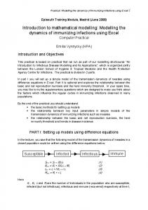


![[PDF] Introduction to Geometrical and Physical Geodesy - Google Sites](https://m.moam.info/img/260x300/pdf-introduction-to-geometrical-and-physical-geode_6477717f097c4786708bb749.jpg)


