Graphical model 是機率理論(probability theory)與圖形理論(graph theory)的結. 合
,他們提供處理不 ... 兩個:灑水器打開(S=true)或下雨(R=true)。它們之間的關係 ...
An introduction to graphical models D91922016 朱威達 1. 介紹 Graphical model 是機率理論(probability theory)與圖形理論(graph theory)的結 合,他們提供處理不確定性(uncertainty)與複雜度(complexity)的工具,在工程問 題中扮演重要的角色。Graphical model 的基本概念在於一個複雜的系統可由較簡 單的零件組成。機率理論讓我們可描述這些零件的數學/相依特性,而圖形理論 則讓我們以直覺的方式指定零件之間的關係。 以下從幾個觀點來說明 graphical model: (1) 表現(representation):一個 graphical model 如何簡潔地表現一個聯合機率 分佈(joint probability distribution)? (2) 推論(inference):如何在給定一些觀察之後推論出系統中未知部份的狀 態? (3) (4) (5)
學習(learning):如何推斷系統的結構(structure)與參數(parameter)? 決定理論(decision theory):如何根據 graphical model 推論出來的結果做 出行動? 應用(application):graphical model 可用於那些應用?
2. 表現 (representation) 若我們有N個binary random variables,要描述P(X1, X2, …, XN)需要O(2N)個參 數。Graphical model可大幅減低所需的參數數量,讓推論與學習變得有效率。 有兩種 graphical model:directed and undirected graphical model。Directed graphical model 又稱為 Bayesian network (BN)、belief network、generative model、 causal model 等。Undirected graphical model 又稱為 Markov network 或 Markov random field (MRF)。 2.1 Directed graphical model 在 directed graphical model 中,有個箭頭從 node A 到 node B 代表 A“造成" (cause) B。舉例言之,如圖一所示,“草地是濕的(grass is wet)"的原因可能有 兩個:灑水器打開(S=true)或下雨(R=true)。它們之間的關係可用一個條件機率表 (conditional probability table, CPT) 來 描 述 。 比 如 說 , 我 們 可 以 看 到 P(W=true|S=true,R=true) = 0.9。 從此圖中我們也可看到某些事情之間是獨立的:在給定 parent 的情況下,某 個 node 與其他 ancestor 無關。此稱為 conditional independent relationship,而 Bayesian network 很適合用於描述這樣的關係。現在我們來看此圖的 joint probability distribution (JPD)。根據 chain rule,它可重新寫成:
圖一、Bayesian network 的例子
P ( C , S , R,W ) = P ( C ) × P ( S C ) × P ( R C , S ) × P (W C , S , R ) 根據 conditional independent relationship,它可改成:
P ( C , S , R,W ) = P ( C ) × P ( S C ) × P ( R C ) × P (W S , R ) 由此我們可以看到它所需要的參數從O(2N)降為O(N2K),其中K是進入點最多 的那個node的進入點個數。
Directed graphical model可有許多變型,可描述許多機率模型或系統,包括 factor analysis、principal component analysis、independent component analysis、 hidden Markov model (HMM) 等。如圖二所示,方形 node 代表 discrete random variable,圓形則為continuous random variable。白色node代表狀態未知(hidden), 而灰色node代表observation。HMM的其中一個重要問題即為從observation推論出 hidden state。其JPD的算法根據此graphical model的表示可寫成右邊的算式。請注 意除了第一個state之外(Q1),之後的state只與前一個state有關,此即為前面提到 的conditional independence relationship。
Q1
Q2
Q3
Q4
4
P ( Q, Y ) = P ( Q1 ) P (Y1 Q1 ) ∏ P ( Qt Qt −1 ) P (Yt Qt ) t =2
Y1
Y2
Y3
Y4
Transition probability Observation probability
圖二、以 graphical model 來表示 hidden Markov model
2.2 Undirected graphical model 若是 edge 無方向性,則為 undirected graphical model,常用於 computer vision 的研究中。在 undirected graphical model 中的 JPD 定義為圖中所有最大 clique 的 potential function 相乘,其中所謂的 potential function 可根據不同問題而有不同定 義。以圖三為例,此圖的 JPD 可寫成:
1 ϕ A ( x1 , x2 , x3 ) ϕ B ( x2 , x3 , x4 ) Z 其為兩個 maximal cliques 的 potential function 相乘再做 normalization。 P ( x1 , x2 , x3 , x4 ) =
X1
X2
X3
X4
圖三、Undirected graphical model 的例子。
3. 推論 (inference) 推論的主要目標是在給定已觀測得的值(observation)之下,推論出隱含(hidden) 於系統中造成此種觀測值的原因。如圖一的例子所示,如果我們看到草地是濕的 (W=true),則造成此後果的原因比較有可能是那一個?我們可根據 chain rule 與 機率轉換計算而得: P ( R = 1, W = 1) P ( R = 1 W = 1) = = P (W = 1) P ( S = 1, W = 1) P ( S = 1 W = 1) = = P (W = 1) P (W = 1) =
∑ P ( C = c, S = s, R = 1,W = 1) c,s
P (W = 1)
∑ P ( C = c, S = 1, R = r ,W = 1) c ,r
P (W = 1)
=
0.4581 = 0.708 0.6471
=
0.2781 = 0.430 0.6471
∑ P ( C = c, S = s, R = r ,W = 1) = 0.6471
c , s ,r
由此可知其實是下雨造成草地濕的機率較高。雖然此作法可計算出結果,但 在計畫 P(W=1)時需要將指數量(exponential number)的參數變化都考慮進去。此計 算複雜度極高。因此我們想利用 graphical model 的結構與 conditional independence relationship 將計算次數降低,此程序即為所謂的變數消去(variable elimination)。
3.1 變數消去(Variable Elimination) 我們考慮上個例子的 normalization term,P(W=1)。我們可將它寫成:
P (W = w ) = ∑∑∑ P ( C = c, S = s, R = r , W = w ) c
s
r
= ∑∑∑ P ( C = c ) × P ( S = s C = c ) × P ( R = r C = c ) × P (W = w S = s, R = r ) c
s
r
Variable elimination 的主要概念是將 summation 越往算式裡面推越好。上面的 式子可改成: P (W = w ) = ∑ P ( C = c ) ∑ P ( S = s C = c ) ∑ P ( R = r C = c ) × P (W = w S = s, R = r ) c
s
r
當我們先處理最裡面的兩個 term 之後,此式子可改成:
P (W = w ) = ∑ P ( C = c ) ∑ P ( S = s C = c ) T1 ( c, w, s ) c
s
同理,它可再寫成: P (W = w ) = ∑ P ( C = c ) T2 ( c, w ) c
如此作法可大幅減少加法與乘法的次數,達到降低 complexity 的目的。 雖然利用 graphical model 的 structure 與 conditional independence 可降低計算 的複雜度,在很多系統裡仍因變數太多或彼此之間關係不易定義而使得 JPD 很 難計算。因此,有許多 approximate inference 的方法被提出,包括 Monte Carlo methods,variational methods,以及 loopy belief propagation 等。
4. 學習 (learning) 在 graphical model 中的學習可能意謂著學習 model 的 structure,參數,或兩 者皆是。我們可根據是否有完整的系統觀測值(observation)與是否知道 model 的 結構(structure)來區分學習演算法(learning algorithm)的種類。 Observability Structure
Full
Partial
Known
Closed form
EM
Unknown
Local search
Structural EM
表一、學習演算法的分類。
4.1 Known structure, full observability 如果我們知道 model structure ,也可觀測到所有的系統值,則 condition probability table 可從各事件發生的次數比例中得到。以前述的例子來說,只要計 算下雨與灑水器開關的次數與草地濕的次數比例即可。也就是:
PˆML (W = w S = s, R = r ) =
# (W = w S = s, R = r ) # ( S = s, R = r )
# ( S = s, R = r ) = # (W = 0, S = s, R = r ) + # (W = 1, S = s, R = r )
4.2 Known structure, partial observability 如果只知道 model structure 而沒有所有的觀測值,則利用 EM algorithm (expectation maximization algorithm)來預估 model parameters。其中 E step 做的是 利用推論演算法(inference algorithm)來預估觀測值。M step 則是根據這些預估的 觀測值找到使整體機率最高的參數。 另 外 還 有 “ unknown structure, full observability " 與 “ unknown structure, partial observability"的情況。許多細節仍是新興的研究課題。 根據 graphical model 的描述與輸出的機率,我們可考慮在不同情況下給定不 同的 cost 來輔助我們做最後的決策。
5. 應用 (application) 許多可由 graphical model 描述的系統或演算模型已廣泛應用於各個研究領 域。如常用於語音辨識的 HMM,用於追蹤的 Kalman filter,用於資料分析的 principal component analysis,用於機器學習的 Bayesian network 等等。Graphical model 是一個非常通用且極具理論基礎的研究工具與課題。 References [1] K. Murphy, An introduction to graphical models, http://www.cs.ubc.ca/~murphyk/Papers/intro_gm.pdf [2] M. I. Jordan and Y. Weiss, Graphical models: Probabilistic inference. In M. Arbib (Ed.), The Handbook of Brain Theory and Neural Networks, 2nd edition. Cambridge, MA: MIT Press, 2002. [3] http://www.cs.ubc.ca/~murphyk/Bayes/bnintro.html Related tools http://www.cs.ubc.ca/~murphyk/Software/