An introduction to integrable techniques for one

Fabio Franchini Ruđer Bošković Institute Bijenčka cesta 54, 10000 Zagreb, Croatia SISSA Via Bonomea 265, 34136, Trieste, Italy

An introduction to integrable techniques for one-dimensional quantum systems June 22, 2017

Contents

1

The XY Chain . . . . . . . . . . . . . . . . . . . . . . . . . . . . . . . . . . . . . . . . . . . . . . . . . . . . . . . . . . . . . . . . . . . . . . . 1.1 Introduction and motivations . . . . . . . . . . . . . . . . . . . . . . . . . . . . . . . . . . . . . . . . . . . . . . . . . . . . . . . 1.2 Diagonalization of the Hamiltonian . . . . . . . . . . . . . . . . . . . . . . . . . . . . . . . . . . . . . . . . . . . . . . . . . . 1.2.1 Even particle number . . . . . . . . . . . . . . . . . . . . . . . . . . . . . . . . . . . . . . . . . . . . . . . . . . . . . . . . 1.2.2 Odd particle number . . . . . . . . . . . . . . . . . . . . . . . . . . . . . . . . . . . . . . . . . . . . . . . . . . . . . . . . . 1.3 The Phase-Diagram . . . . . . . . . . . . . . . . . . . . . . . . . . . . . . . . . . . . . . . . . . . . . . . . . . . . . . . . . . . . . . . . 1.4 The correlation functions . . . . . . . . . . . . . . . . . . . . . . . . . . . . . . . . . . . . . . . . . . . . . . . . . . . . . . . . . . . 1.5 The Kitaev chain . . . . . . . . . . . . . . . . . . . . . . . . . . . . . . . . . . . . . . . . . . . . . . . . . . . . . . . . . . . . . . . . . .

3 3 4 7 7 9 10 13

2

The Lieb-Liniger Model . . . . . . . . . . . . . . . . . . . . . . . . . . . . . . . . . . . . . . . . . . . . . . . . . . . . . . . . . . . . . 2.1 Introduction . . . . . . . . . . . . . . . . . . . . . . . . . . . . . . . . . . . . . . . . . . . . . . . . . . . . . . . . . . . . . . . . . . . . . . 2.2 Generalities on the Bethe Ansatz approach . . . . . . . . . . . . . . . . . . . . . . . . . . . . . . . . . . . . . . . . . . . 2.3 The two-particle problem . . . . . . . . . . . . . . . . . . . . . . . . . . . . . . . . . . . . . . . . . . . . . . . . . . . . . . . . . . . 2.4 Bethe Ansatz Wavefunction . . . . . . . . . . . . . . . . . . . . . . . . . . . . . . . . . . . . . . . . . . . . . . . . . . . . . . . . . 2.4.1 Bound States . . . . . . . . . . . . . . . . . . . . . . . . . . . . . . . . . . . . . . . . . . . . . . . . . . . . . . . . . . . . . . . 2.5 The Bethe Equations . . . . . . . . . . . . . . . . . . . . . . . . . . . . . . . . . . . . . . . . . . . . . . . . . . . . . . . . . . . . . . 2.6 The thermodynamic limit . . . . . . . . . . . . . . . . . . . . . . . . . . . . . . . . . . . . . . . . . . . . . . . . . . . . . . . . . . 2.7 Some formalities on Integral Equations . . . . . . . . . . . . . . . . . . . . . . . . . . . . . . . . . . . . . . . . . . . . . . . 2.8 Elementary excitations . . . . . . . . . . . . . . . . . . . . . . . . . . . . . . . . . . . . . . . . . . . . . . . . . . . . . . . . . . . . . 2.9 Thermodynamics of the model: the Yang-Yang equation . . . . . . . . . . . . . . . . . . . . . . . . . . . . . . . . 2.9.1 T → 0+ . . . . . . . . . . . . . . . . . . . . . . . . . . . . . . . . . . . . . . . . . . . . . . . . . . . . . . . . . . . . . . . . . . . . 2.9.2 c → ∞ . . . . . . . . . . . . . . . . . . . . . . . . . . . . . . . . . . . . . . . . . . . . . . . . . . . . . . . . . . . . . . . . . . . . . 2.9.3 c → 0+ . . . . . . . . . . . . . . . . . . . . . . . . . . . . . . . . . . . . . . . . . . . . . . . . . . . . . . . . . . . . . . . . . . . . .

15 15 16 17 18 19 20 22 24 25 30 33 34 34

3

The Heisenberg chain . . . . . . . . . . . . . . . . . . . . . . . . . . . . . . . . . . . . . . . . . . . . . . . . . . . . . . . . . . . . . . . . 3.1 Definition of the model . . . . . . . . . . . . . . . . . . . . . . . . . . . . . . . . . . . . . . . . . . . . . . . . . . . . . . . . . . . . . 3.2 The vacuum state and the magnon basis . . . . . . . . . . . . . . . . . . . . . . . . . . . . . . . . . . . . . . . . . . . . . 3.3 The two-body problem . . . . . . . . . . . . . . . . . . . . . . . . . . . . . . . . . . . . . . . . . . . . . . . . . . . . . . . . . . . . . 3.4 The Bethe Solution . . . . . . . . . . . . . . . . . . . . . . . . . . . . . . . . . . . . . . . . . . . . . . . . . . . . . . . . . . . . . . . . 3.4.1 String solutions . . . . . . . . . . . . . . . . . . . . . . . . . . . . . . . . . . . . . . . . . . . . . . . . . . . . . . . . . . . . . 3.5 The Ferromagnetic case: J = 1 . . . . . . . . . . . . . . . . . . . . . . . . . . . . . . . . . . . . . . . . . . . . . . . . . . . . . . 3.6 The Anti-Ferromagnetic case: J = −1 . . . . . . . . . . . . . . . . . . . . . . . . . . . . . . . . . . . . . . . . . . . . . . . . 3.7 Interaction with a magnetic field . . . . . . . . . . . . . . . . . . . . . . . . . . . . . . . . . . . . . . . . . . . . . . . . . . . .

35 35 36 36 39 41 44 45 51

4

The XXZ Chain . . . . . . . . . . . . . . . . . . . . . . . . . . . . . . . . . . . . . . . . . . . . . . . . . . . . . . . . . . . . . . . . . . . . . 4.1 Generalities . . . . . . . . . . . . . . . . . . . . . . . . . . . . . . . . . . . . . . . . . . . . . . . . . . . . . . . . . . . . . . . . . . . . . . . 4.2 Bethe Ansatz solution . . . . . . . . . . . . . . . . . . . . . . . . . . . . . . . . . . . . . . . . . . . . . . . . . . . . . . . . . . . . . . 4.3 Uni-axial Ferromagnet: ∆ > 1 . . . . . . . . . . . . . . . . . . . . . . . . . . . . . . . . . . . . . . . . . . . . . . . . . . . . . . .

53 53 54 58 vii

viii

Contents

4.3.1 Effect of the magnetic field on the ferromagnet . . . . . . . . . . . . . . . . . . . . . . . . . . . . . . . . . . 4.4 Paramagnetic/Planar Regime: |∆| < 1 . . . . . . . . . . . . . . . . . . . . . . . . . . . . . . . . . . . . . . . . . . . . . . . 4.4.1 Spinon and magnon excitations in the paramagnetic phase . . . . . . . . . . . . . . . . . . . . . . . . 4.4.2 String solutions in the paramagnetic phase . . . . . . . . . . . . . . . . . . . . . . . . . . . . . . . . . . . . . 4.4.3 Effect of the magnetic field on the paramagnet . . . . . . . . . . . . . . . . . . . . . . . . . . . . . . . . . . 4.5 Uni-axial Anti-ferromagnet: ∆ < −1 . . . . . . . . . . . . . . . . . . . . . . . . . . . . . . . . . . . . . . . . . . . . . . . . . 4.5.1 Effect of the magnetic field on the anti-ferromagnet . . . . . . . . . . . . . . . . . . . . . . . . . . . . . .

59 59 60 60 63 68 68

5

Algebraic Bethe Ansatz . . . . . . . . . . . . . . . . . . . . . . . . . . . . . . . . . . . . . . . . . . . . . . . . . . . . . . . . . . . . . . 5.1 Generalities on the algebraic approach . . . . . . . . . . . . . . . . . . . . . . . . . . . . . . . . . . . . . . . . . . . . . . . 5.2 Preliminaries . . . . . . . . . . . . . . . . . . . . . . . . . . . . . . . . . . . . . . . . . . . . . . . . . . . . . . . . . . . . . . . . . . . . . . 5.3 Transfer Matrix for the XXZ chain . . . . . . . . . . . . . . . . . . . . . . . . . . . . . . . . . . . . . . . . . . . . . . . . . . 5.4 The ABA solution . . . . . . . . . . . . . . . . . . . . . . . . . . . . . . . . . . . . . . . . . . . . . . . . . . . . . . . . . . . . . . . . . 5.5 Construction of the operators: the inverse scattering problem . . . . . . . . . . . . . . . . . . . . . . . . . . . 5.6 Scalar products and norms: Slavnov’s and Gaudin’s Formulas . . . . . . . . . . . . . . . . . . . . . . . . . . . 5.7 Algebraic approach to the Lieb-Liniger model: The Lax Representation . . . . . . . . . . . . . . . . . . . 5.8 The Braid Limit . . . . . . . . . . . . . . . . . . . . . . . . . . . . . . . . . . . . . . . . . . . . . . . . . . . . . . . . . . . . . . . . . . . 5.9 A glimpse into Quantum Groups . . . . . . . . . . . . . . . . . . . . . . . . . . . . . . . . . . . . . . . . . . . . . . . . . . . .

69 69 72 73 77 81 82 87 89 90

A

Asymptotic behavior of Toeplitz Determinants . . . . . . . . . . . . . . . . . . . . . . . . . . . . . . . . . . . . . . A.1 Introduction . . . . . . . . . . . . . . . . . . . . . . . . . . . . . . . . . . . . . . . . . . . . . . . . . . . . . . . . . . . . . . . . . . . . . . A.2 The Strong Szegö Theorem . . . . . . . . . . . . . . . . . . . . . . . . . . . . . . . . . . . . . . . . . . . . . . . . . . . . . . . . . A.3 The Fisher-Hartwig Conjecture . . . . . . . . . . . . . . . . . . . . . . . . . . . . . . . . . . . . . . . . . . . . . . . . . . . . . . A.4 Generalized Fisher-Hartwig: Basor-Tracy Conjecture . . . . . . . . . . . . . . . . . . . . . . . . . . . . . . . . . . . A.5 Widom’s Theorem . . . . . . . . . . . . . . . . . . . . . . . . . . . . . . . . . . . . . . . . . . . . . . . . . . . . . . . . . . . . . . . . .

93 93 94 94 95 96

B

Two-Dimensional Classical Integrable Systems . . . . . . . . . . . . . . . . . . . . . . . . . . . . . . . . . . . . . . . 97 B.1 Overview of the approach . . . . . . . . . . . . . . . . . . . . . . . . . . . . . . . . . . . . . . . . . . . . . . . . . . . . . . . . . . 97 B.2 Ice-type models . . . . . . . . . . . . . . . . . . . . . . . . . . . . . . . . . . . . . . . . . . . . . . . . . . . . . . . . . . . . . . . . . . . 98 B.3 The Transfer Matrix and the Yang-Baxter equations . . . . . . . . . . . . . . . . . . . . . . . . . . . . . . . . . . . 100 B.4 T-Q relations . . . . . . . . . . . . . . . . . . . . . . . . . . . . . . . . . . . . . . . . . . . . . . . . . . . . . . . . . . . . . . . . . . . . . 105

C

Field theory and finite size effects . . . . . . . . . . . . . . . . . . . . . . . . . . . . . . . . . . . . . . . . . . . . . . . . . . . C.1 Bosonization . . . . . . . . . . . . . . . . . . . . . . . . . . . . . . . . . . . . . . . . . . . . . . . . . . . . . . . . . . . . . . . . . . . . . . C.2 Conformal Field Theory parameters from Bethe Ansatz . . . . . . . . . . . . . . . . . . . . . . . . . . . . . . . . C.2.1 Sound velocity . . . . . . . . . . . . . . . . . . . . . . . . . . . . . . . . . . . . . . . . . . . . . . . . . . . . . . . . . . . . . . C.2.2 Central Charge . . . . . . . . . . . . . . . . . . . . . . . . . . . . . . . . . . . . . . . . . . . . . . . . . . . . . . . . . . . . . C.2.3 Conformal dimensions from finite size . . . . . . . . . . . . . . . . . . . . . . . . . . . . . . . . . . . . . . . . . . C.3 Bosonization of the Lieb-Liniger model . . . . . . . . . . . . . . . . . . . . . . . . . . . . . . . . . . . . . . . . . . . . . . . C.4 Bosonization of the XXZ model . . . . . . . . . . . . . . . . . . . . . . . . . . . . . . . . . . . . . . . . . . . . . . . . . . . . .

107 107 112 114 114 115 120 122

Index . . . . . . . . . . . . . . . . . . . . . . . . . . . . . . . . . . . . . . . . . . . . . . . . . . . . . . . . . . . . . . . . . . . . . . . . . . . . . . . . . . . . 125 References . . . . . . . . . . . . . . . . . . . . . . . . . . . . . . . . . . . . . . . . . . . . . . . . . . . . . . . . . . . . . . . . . . . . . . . . . . . . . . . 127

Preface

These notes are the write-up and extension of the lectures I gave over a few years for a class on “Introduction to Bethe Ansatz” within the Ph.D. program in Statistical Physics at SISSA (Trieste). They are intended as a guidance to start the study of this extremely rich subject, by favoring a clear and physical introduction to its fundamental ideas, over many mathematical subtleties that populate its formulation. The emphasis on the physical intuition makes these notes suitable also for the scientist who mostly performs numerical simulations, but wants to compare his/her results with exact ones, and to anyone who needs to start reading the literature on Bethe Ansatz and integrable models. Modern physics is all about universality, but we should never forget that universal behaviors emerge from microscopic dynamics and thus solvable models have always played a pivotal role in providing concrete realizations of different phenomenologies to test hypothesis and shaping our intuition. Over the years, integrable models have helped us in constructing better numerical methods and in developing and testing general theories such as Bogoliubov theory for weakly interacting gases, Luttinger liquid, non-linear Lutting liquids and so on. Integrable techniques have witnessed a resurgence in popularity in recent times, mostly due to the outstanding progresses in experimental capabilities, for instance in cold atoms, which disclose the possibility of engineering virtually any desired interaction and geometry [1]. These breakthroughs have in turn stimulated new questions, to address which exact tools are a valuable asset. It is yet not clear which qualitative features separate integrable from non-integrable quantum systems [2]. While in classical physics this distinction is clear, all the proposed answers for the quantum case are somewhat unsatisfactory, although the analysis of out-of-equilibrium settings seems to provide interesting results in this respect [3, 4]. Regardless of these considerations, we know that a small, but interesting, subset of many-body quantum systems is amenable to exact solution. By this, we mean that each eigenstate of such systems can be uniquely characterized by a set of quantum numbers, which curiously seems to be in a one-to-one correspondence with a free fermionic system. This realization allows to classify the states in terms of their elementary excitations (quasi-particles). In this respect it should be stressed that the added value of these techniques does not lie on their bare efficiency (nowadays we have very powerful numerical tools at our disposal), but on the insights they provide to interpret a many-body system (and then to develop even more efficient simulations). The fundamental ingredient responsible for such analytical solution is the fact that any scattering event can be decomposed into a sequence of two-body scatterings, and the ordering in such sequence does not alter the result. This properties means that the fundamental quasiparticle excitations cannot be created, nor destroyed in a scattering event governed by an integrable Hamiltonian. This is the realization behind Bethe’s original ansatz for the solution of the Heisenberg chain and the foundation over which a beautiful mathematical physics construction has been erected. This integrability is a peculiar property only of 1+1-dimensional quantum systems. While for many years the study of Bethe Ansatz was purely theoretically motivated, nowadays we have several systems where the degrees of freedom are effectively confined to move along a line/chain, because the transverse directions are

1

2

Contents

energetically blocked. In some crystalline compounds, for instance, atoms are placed in such a way that their magnetic moments interact preeminently with neighbors in one (or two) directions. In lithography it is possible to realize conducting wires so thin that the transverse component of the electron wavefunction is frozen. Most of all, cold atoms can be manipulated with high precision with external laser beams which allow to confine them in virtually any desired geometry and probe them with remarkable accuracy. There are several excellent sources where to learn about integrable techniques. These notes try to introduce all the basic tools and ideas, while keeping a short, but pedagogical approach. To do so, a small number of examples were selected. We will start with the XY chain, which is essentially a free system with a non-trivial phase diagram and the prototypical model to address a variety of questions. Next we will solve the LiebLiniger model of one-dimensional bosons with contact interaction. This model has the merit of being very close to experimental relevance and allows for a clear introduction of the coordinate Bethe Ansatz solution to study its zero and finite temperature thermodynamics. We will then move to the Heisenberg spin-1/2 chain and the XXZ chain, which will be our reference model to introduce more advanced topics such as the issue of string solutions and the algebraic Bethe Ansatz approach. To better introduce the latter, we also briefly explain the solution of the two-dimensional classical 6-vertex model in one of the appendices, since these techniques were instrumental in the realization of the algebraic structure behind integrability. The other appendices contain a collection of results on Toeplitz determinants (which are relevant for the XY chain) and a digression on the relation between Bethe Ansatz solutions and the field theories describing the low energy properties of these models. A noticeable absence among the topics covered is that of the nested Bethe Ansatz for systems with internal degrees of freedom. We refer the interested reader to [5] for an exhaustive treatment of the 1D Hubbard model, as the prototypical, and experimentally relevant, example of such systems. I wish to thank Giuseppe Mussardo for the opportunity of teaching the class that pushed me to write these notes and deepen my understanding of the subject and to all my friends and colleagues for their advices and insights. I am also grateful to Guillaume Lang for his thorough reading of the the first version of this manuscript and for his comments and corrections.

Chapter 1

The XY Chain

Abstract The XY chain in a transverse magnetic field is a generalization of the 1D Ising model, with whom it shares the property of being essentially a free system. Its rich and non-trivial phase-diagram and the possibility of calculating virtually every quantity have rendered it a reference model to understand new effects or to test hypotheses. After a brief introduction in Sec. 1.1, in Sec. 1.2 we review its standard mapping to free fermions, paying particular attention on the interplay between the two parity sectors of the Hilbert space to understand the Z2 symmetry breaking. In Sec. 1.2 we discuss the phase diagram and in Sec. 1.4 we show how to calculate some basic correlation functions and we discuss their behavior in the different phases. Finally, in Sec. 1.5 we comment on the relation between the Ising model and the Kitaev chain, which provides a natural interpretation of the Z2 symmetry in terms of Majorana boundary modes.

1.1 Introduction and motivations The One-Dimensional XY model in a transverse magnetic field is arguably the simplest non-trivial integrable model. Its simplicity derives from the fact that its excitations are non-local free fermions. This non-locality is the source of the non-trivial 2-parameters phase diagram, characterized, at zero temperature, by two Quantum Phase Transitions (QPTs): one belonging to the universality of the anti-ferromagnetic Heisenberg chain (aka, the XX model, with conformal charge c equal to 1) and the other to the Ising model (c = 1/2). The Hamiltonian of the XY model can be written as H=J

N h X j=1

N i JX 1+γ 1−γ y y x x (1 + γ) Sjx Sj+1 +(1 − γ) Sjy Sj+1 +h Sjz = σjx σj+1 + σjy σj+1 + h σjz , 2 j=1 2 2

(1.1) where σjα , with α = x, y, z, are the Pauli matrices which describe spin-1/2 operators on the j-th lattice site of a chain with N sites. This Hamiltonian describes a one-dimensional lattice, where a 3D spin variable lives on every lattice point. The spins interact with their nearest neighbor in an anisotropic way (parametrized by γ), so that the interaction between their z-components (that is, the direction of an external magnetic field h) can be neglected. This model was first introduced and solved in the case of zero magnetic field h by Lieb, Schultz and Mattis in [6] and in [7, 8] with a finite external field. The fundamental correlation functions were calculated in [9]. More complicated correlators like the Emptiness Formation Probability [10, 11, 12] and the Von Neumann [13, 14] and Renyi [15] entanglement entropies were calculated more recently, as well as several out-of-equilibrium properties [16]. Virtually all static correlation functions of the model can be expressed as determinants of matrices with a special structure, known as Toeplitz matrices [17]. The asymptotic behavior of Toeplitz determinants can be studied using fairly sophisticated mathematical techniques or just by relying on known theorems, such as the Szegö Theorem, the Fisher-Hartwig conjecture, Widom’s theorem and so on ...[18, 19]

3

4

1 The XY Chain

The phase diagram of this model is parametrized by the anisotropy parameter γ capturing the relative strength of interaction in the x and y components and by the external magnetic field h, directed along the transverse z-axis. We take these parameters to be dimensionless and from now on we set the energy-scale defining parameter as J = −1 (that is, we will consider an easy-plane ferromagnet). The model has obvious symmetries: a rotation by π/2 along the z-axis interchanges the x and y spin interactions and is equivalent to γ → −γ, while a reflection of the spin across the x − y plane is compensated by h → −h: thus we will concentrate only on the first quadrant of the phase diagram (γ ≥ 0, h ≥ 0), since the rest of the phase diagram is related by the above symmetries. The two quantum phase transitions, that is, the parameters for which the spectrum becomes gapless, are located on the isotropic line γ = 0 (|h| ≤ 1), and at the critical magnetic field |h| = 1. We remark that for γ = 0 the Hamiltonian reduces to the isotropic XX model , i.e. the ∆ = 0 limit of the XXZ chain , which will be studied in chapter 4. For γ = ±1, we recover the 1D Quantum Ising model . These two cases correspond to the two competing universality classes which can be realized by the XY chain. The isotropic line corresponds to free fermions hopping on a lattice and thus belong to a c = 1 Conformal Field Theory (CFT) universality . The critical magnetic field h = ±1 is an Ising transition, that is, a transition from a doubly degenerate ground state (for |h| < 1) to a single ground state system (for |h| > 1). It is the same as the classical phase transition occurring in the two-dimensional Ising model [20]. In fact, the latter can be solved through its transfer matrix, which takes the same form as the exponential of (1.1), with the magnetic field taking the role of the temperature [21]. The order parameter of this transition for the classical model is the magnetization and in the quantum case it is the magnetization along the x-axis. Thus, consistently with the Z2 symmetry of the model, hσ x i goes from vanishing for |h| > 1, to finite ±mx for |h| < 1. The latter behavior is exemplified by the (γ, h) = (1, 0) point, where the two ground states are |GS1 i = | → → → . . .i =

N Y 1 √ | ↑j i + | ↓j i , 2 j=1

|GS2 i = | ← ← ← . . .i =

N Y 1 √ | ↑j i − | ↓j i , (1.2) 2 j=1

where | ↑j i (| ↓j i) indicates the state with positive (negative) projection of the spin along the z-axis at the j-th lattice point. We see that these states have hσ x i = ±1. The exact degeneracy between the two ground states is in general lifted away from the point (γ, h) = (1, 0) for finite chains, and is recovered in the whole phase only in the thermodynamic limit. However, as noted in [22], the factorized structure (1.2) for the degenerate ground states propagates on the line γ 2 + h2 = 1, where the two ground states can be written explicitly as |GS1 i =

N Y

cos θ | ↑j i + sin θ | ↓j i

,

j=1

|GS2 i =

N Y

cos θ| ↑j i − sin θ | ↓j i

,

(1.3)

j=1

where cos2 (2θ) = (1 − γ)/(1 + γ). Remarkably, on this line the degeneracy is exact for any length of the chain. We see that along this line, the spins, initially aligned along the x-axis, progressively acquire a growing positive z component and eventually merge into a perfectly polarized state at the point (γ, h) = (0, 1). This is the bicritical point of junction between the two critical lines γ = 0 and h = 1 and is quite special, in that the spectrum becomes perfectly quadratic. Thus, at this point the model is critical, but not conformal, since its dynamical critical exponent is equal to 2.

1.2 Diagonalization of the Hamiltonian α The standard prescription to diagonalize (1.1) assumes periodic boundary conditions σj+N = σjα . It is quite inconvenient to work directly with spin operators, since on each site they behave fermionically (in that they span a finite-dimensional Fock space), but between sites they obey bosonic commutation relations. In one

1.2 Diagonalization of the Hamiltonian

5

dimension, however, this problem can be circumvented by mapping the spins into either fermionic or bosonic operators: in the first case, one needs to introduce a strong repulsive interaction to truncate the Hilbert space, while the price for the latter choice is that the mapping is highly non-local. We pursue the latter. Following [6], we reformulate the Hamiltonian (1.1) in terms of spinless fermions ψj by means of a JordanWigner transformation : iπ

σj+ = e

P l 0

(1.30)

and thus (1.29) is the same as (1.20). Hence, the Hilbert space is populated like in the previous case by successive applications of pairs of operators χ†q χ†q0 or χ†q χ0 to |GSi− . Note that in the thermodynamic limit these states and those generated in the even excitation sector intertwine and thus one can effectively forget about the separation into the two sectors.

1.2.2.2 Ordered Phase For h < 1 h − 1 = −ε(0) < 0

(1.31)

and thus the presence of a zero-mode lowers the energy of the system (notice that, because of our normal1 † 1 ization for the Fourier modes N χ0 χ0 − 2 χ†0 = χ†0 ). The energy of (1.27) for h < 1 is E0− =

N −1 1 1 X (h − 1) − ε 2 2 q=1

2π N q

=−

N −1 1 X ε 2 q=0

2π N q

N →∞ N → − 2

Z 0

2π

dq ε(q) , 2π

(1.32)

where the last expression holds in the thermodynamic limit N → ∞. We see that in the thermodynamic limit the lowest energy state in this sector (with a zero mode) and the ground state with no excitation in the even particle sector become degenerate (E0+ = E0− ). It can be proven, see for instance [24], that the gap between |GSi− and |GSi+ closes exponentially in the system size N (with frequent exchanges in which out of the two |GSi± has the lowest energy). Moreover, it is also clear that each state of the even excitation sector lies exponentially close to one state of the odd sector (for instance the states χ†q+1/2 χ†q0 +1/2 |GSi+ and χ†q χ†q0 |GSi− , or χ†q+1/2 χ†1/2 |GSi+ and χ†q χ0 |GSi− ). We have thus shown that the special role of the zero mode renders the whole spectrum of the ordered phase doubly degenerate, while this degeneracy disappears for h > 1. 3

For even size lattices (N = 2M ) the same holds for the q = M component (i.e. a π-momentum particle), which is the contribution to single out for antiferromagnetic coupling J < 0 in (1.1). More interesting is the case of odd-size lattices with antiferromagnetic coupling: this setting introduces a frustration which renders the whole region |h| < 1 gapless [23]

1.3 The Phase-Diagram

9

1.3 The Phase-Diagram As we mentioned, the zero temperature phase diagram is quite interesting, due to the presence of two different quantum phase transitions. It is easy to find them, since they are the points in the (γ, h) plane where the minimum of the spectrum (1.21) is zero. Thus, at these points the mass gap vanishes and the gapless low energy excitations determine a scale-invariant behavior. From (1.21) we see that this happens for γ = Ising 0, |h| < 1 (isotropic XX model: c = 1 CFT) and for |h| = 1 (critical magnetic field: c = 1/2 CFT). In Fig. 1.1 we draw the phase diagram “Disordered” of the XY model for γ ≥ 0 and h ≥ 0. It shows the critical lines γ = 0 and h = 1 and the line γ = 1 corresponding to the Ising model in 1 transverse magnetic field and the line γ 2 +h2 = 1 on which the wave function of the ground state is factorized into a product of single spin “Ordered” states (1.3) [22]. We already determined that the h = 1 line “Oscillatory” separates a doubly degenerate phase from a non-degenerate one and thus corresponds to the spontaneous breaking of Z2 . The low energy excitations close to h = 1 have vanishing momen0 g 1 tum. Crossing the γ = 0 lines, the role of x and y gets inverted (the (non-)vanishing order parameters switch from mx to my ). Approaching Fig. 1.1 Phase diagram of the XY Model (only γ ≥ 0 and h ≥ 0 this QPT, there are two types of low energy is shown). The model is critical for h = 1 and for γ = 0 and h < 1 Ising Model in transverse field states, with momenta approximately equal to (in bold red). The line γ = 12 is the (dotted line). On the line γ + h2 = 1 the ground states can be ± arccos h. We will understand better the dif- factorized as a product of single spin states (blue dashed line). ferent phases and the nature of their low-energy excitations in the next section. The finite temperature partition function of the XY model for h < 1 is # "N −1 −1 NY X π π 2π 1 −βE0+ Y q+ −βε q+ −βε( 2π −βEi N N) N) + 1−e (N e 1+e Z= e = 2 q=0 q=0 "N −1 # −1 NY 2π 1 −βE0− Y −βε( 2π q q −βε ) + N + e 1+e 1−e (N ) 2 q=0 q=0 (N −1 NY ) −1 Y β β π π ε 2π + sinh ε 2π = 2N −1 cosh N q+ N N q+ N 2 2 q=0 q=0 (N −1 NY ) −1 Y β β +2N −1 cosh ε 2π + sinh ε 2π , (1.33) N q N q 2 2 q=0 q=0

h

where the terms with a minus sign within each square bracket kill states with the wrong parity of excitations in each sector. Taking the thermodynamic limit, the free energy per site is: " # Z π N −1 Y 1 1 1 1 β 1 1 β 2π F = − lim ln Z = − ln 2 − ln cosh ε(ω) dω − lim ln 1 + tanh ε N q , β N →∞ N β πβ 0 2 β N →∞ N 2 q=0 (1.34)

10

1 The XY Chain

where the last term, encoding the degeneracy of the model, is clearly negligible in the thermodynamic limit. For h > 1 (N −1 NY ) −1 Y β 2π β 2π N −1 π π Z= 2 cosh ε q+ N + ε q+ N sinh 2 N 2 N q=0 q=0 (N −1 NY ) −1 Y β 2π β 2π N −1 . (1.35) +2 cosh q − sinh q ε ε 2 N 2 N q=0 q=0 and the free energy per site in the thermodynamic limit is Z π 1 β 1 F = − ln 2 − ln cosh ε(ω) dω . β πβ 0 2

(1.36)

Clearly, from the partition function we can derive the whole thermodynamics of the model, which is essentially that of free fermions.

1.4 The correlation functions In this section we review the derivation of the fundamental correlators in the ground state |GSi+ at zero temperature, following McCoy and co-authors [9]. In the ordered phase, the ground state of the XY model breaks Z2 symmetry (that is, is not an eigenstate √ of the parity operator (1.6)) and thus the true ground state of the model is |GSi = (|GSi+ ± |GSi− ) / 2. However, all parity-conserving operators have the same expectation values for |GSi+ as with respect to |GSi. We will thus henceforth drop the reference to the sector. Since the model is quadratic, all correlation functions can be expressed in terms of two-point functions using Wick’s theorem. Let us thus concentrate on the latter. Using (1.22) we have hGS|χq χ†k |GSi = N δk,q , hGS|χq χk |GSi = 0 ,

hGS|χ†q χk |GSi = 0 ,

(1.37)

hGS|χ†q χ†k |GSi

(1.38)

=0.

As (1.24) shows, this state is far from a vacuum, empty of fermions, as a consequence of the superconducting terms in (1.14). Using (1.16), in terms of the physical fermions we have 1 − cos 2ϑq N δk,q , 2 sin 2ϑq hGS|ψq ψk |GSi = − N δ−k,q , 2

hGS|ψq† ψk |GSi =

1 + cos 2ϑq N δk,q , 2 sin 2ϑq hGS|ψq† ψk† |GSi = N δ−k,q . 2 hGS|ψq ψk† |GSi =

(1.39) (1.40)

The two-point fermionic correlators are obtained by Fourier transform. In the thermodynamic limit they read [6, 9] Fjl ≡ ihGS|ψj ψl |GSi = Gjl ≡ hGS|ψj ψl† |GSi =

−ihGS|ψj† ψl† |GSi Z 0

2π

Z = 0

2π

dq sin 2ϑ(q) iq(j−l) e , 2π 2

dq 1 + cos 2ϑ(q) iq(j−l) e , 2π 2

(1.41) (1.42)

γ sin q where the function ϑ(q) ≡ 12 arctan h−cos q is the continuum limit of (1.18). If our starting point was the spinless fermions Hamiltonian (1.10), these would be all we need. However, what we are really after are the spin-spin correlation functions, for which we have to take into account the non-local effects of the JordanWigner transformation.

1.4 The correlation functions

11

Thus, we follow [6] and introduce the following expectation values ν ρνlm ≡ hGS |σlν σm | GSi

ν = x, y, z,

which can be written in terms of spin lowering and raising operators as + − ρxlm = hGS σl+ + σl− σm GSi , + σm + + y − − ρlm = −hGS σl − σl σm − σm GSi , + − z + − ρlm = hGS 1 − 2σl σl 1 − 2σm σm GSi .

(1.43)

(1.44) (1.45) (1.46)

The key observation is that the product of two Jordan-Wigner strings is the identity, since each of them measure the magnetization parity. Thus, for instance, we can use (1.4) on ρxlm to get + − ρxlm = hGS σl+ + σl− σm GSi + σm m−1 Y † 1 − 2ψj† ψj ψm + ψm |GSi = hGS| ψl† + ψl j=l

m−1 Y † = hGS| ψl† − ψl 1 − 2ψj† ψj ψm + ψm |GSi

j=l+1

m−1 Y † † = hGS| ψl† − ψl ψj + ψj ψj† − ψj ψm + ψm |GSi,

(1.47)

j=l+1

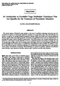
where we have used the identities P P iπ ψ † ψl −iπ ψ † ψl l 0 and h2 + γ 2 > 1, λ+ is closer to the circle and ρx (n) approaches the saturation exponentially. For h2 + γ 2 < 1 both λ± acquire an imaginary part and become complex conjugated. Thus, they both contribute to the asymptotic behavior and the correlation functions develop a periodic modulation (the two contributions can be traced on the existence of two distinct minima in the single particle spectrum). Hence, the name of “oscillatory phase”. Going to negative magnetic field, the role of λ+ and λ− gets inverted, while crossing the line γ = 0 one should exchange λ± with λ−1 ± . Note that the spontaneous magnetization is inferred from the asymptotic behavior of the two-point function ρx (∞). It would be desirable to calculate directly hσ x i. However, a non-zero expectation value for such operator requires that the bra and the ket belong to different parity sectors and, so far, nobody has devised a method to perform such calculation directly.

1.5 The Kitaev chain

13

Fig. 1.2 Cartoon of the positions of the two length-scale parameters of the models λ± (1.58) with respect to the unit circle (in dashed blue). ρx (n) '

n→∞ “Disordered Phase”

XD

h>1 “Ising Transition”

Cx

h=1
0.

2.5 The Bethe Equations In order to quantize the system, we put it in a box of finite length L (which we can take to infinity in the end). We impose periodic boundary conditions on the walls of this box, effectively considering a ring: Ψ (x1 , x2 , . . . , xj + L, . . . , xN ) = Ψ (x1 , x2 , . . . , xj , . . . , xN ) ,

j = 1, . . . , N .

(2.30)

Let us consider the “first” particle in the system (note that, on a circle, any particle can be taken as the first). The periodic boundary condition (2.30) relates a given simplex with that in which the first particle has been moved to be the last one. From a formal point of view, this permutation can be realized as a sequence of two-body permutations, in which particle 1 is first exchanged with particle 2, then with particle 3 and so on. From a physical viewpoint, taking a particle around the circle means that it has scattered across all other particles in the system. Through all these scattering events it acquires a phase equal to the sum of the scattering phases associated with each scattering event plus the dynamical phase accumulated through the

2.5 The Bethe Equations

21

motion (namely its quasi-momentum times L). To satisfy periodic boundary conditions, the sum of these phase contributions has to add up to an integer multiple of 2π. We formalize the consistency relations imposed by the periodic boundary conditions by relating the permutation in real space with one in quasi-momenta space, as we commented above. Denoting the permutation that brings the first element to be the last as R {1, 2, . . . , N } = {2, 3, . . . , N, 1}, we have AP (Q) = AP (RQ) eikP1 L = ARP (Q) eikP1 L .

(2.31)

Using (2.18) this condition can be written as ikj L

e

N Y Y kj − kl + i c = (−1)N −1 eiθ(kj −kl ) , = kj − kl − i c

j = 1, . . . , N ,

(2.32)

l=1

l6=j

which shows how the dynamical phase on the LHS has to match the scattering phase on the RHS. Taking the logarithm we get kj L = 2π I˜j + (N − 1)π − 2

N X l=1

= 2πIj +

N X

arctan

kj − kl c

θ(kj − kl ) ,

(2.33)

l=1

where the I˜j are a set of integers which define the state. In the second line we introduced a new set Ij : they are integers if the number of particles N is odd and half-integers if N is even3 . The Ij ’s are called quantum (or Bethe) numbers and they characterize uniquely the state. Notice that if two quantum numbers are equal Ij = Il , their corresponding quasi-momenta also coincide kj = kl . Since, as we commented above, in such cases the Bethe wavefunction (2.16) vanishes, we conclude that only sets of distinct Bethe numbers correspond to physical solutions. The (2.33) are the Bethe equations, a set of N coupled algebraic equations in N unknowns, the kj . For c → ∞ we have hard-core bosons: θ(k) → 0 and kj = 2πIj /L. Since they have to be all different, the ground state which minimizes the energy and momentum (2.19) is given by a symmetric distribution of quantum numbers without holes (a Fermi sea distribution): Ij = −

N +1 +j , 2

j = 1...N .

(2.34)

If we now decrease the coupling c from infinity, we slowly turn on a scattering phase so that, for fixed Ij , the solution kj to the Bethe equations (2.33) will move from the original regular distribution. Since there cannot be a level crossing (there is no symmetry to protect a degeneracy and accidental ones cannot happen in an integrable model), the state defined by (2.34) will remain the lowest energy state for any interaction strength (note that, changing c changes the quasi-momenta kj , but cannot change the quantum number, because they are quantized). It is possible to prove this statement, the non-degenerate condition and the uniqueness of the solution obtained through Bethe Ansatz, but we refer to [41] for such rigorous proofs. Each choice for the quantum numbers yields an eigenstate, provided that all Bethe numbers are different. This rule confers a fermionic nature to the Bethe Ansatz solution (in quasi-momentum space!), even if the underlying system is composed by bosons (in the real space) as in this case. P Finally, please note that since θ(−k) = −θ(k), the momentum of the system is K = 2π j Ij . So the L momentum is quantized and does not vary as the coupling constant is varied.

3

This is equivalent to the different quantization of the momenta we found in the chapter 1 for the XY model.

22

2 The Lieb-Liniger Model

2.6 The thermodynamic limit If we order the Bethe numbers Ij ’s (and therefore the momenta kj ’s) in increasing order, we can write the Bethe Equations (2.33) as N 1X kj − θ(kj − kl ) = y(kj ) (2.35) L l=1

where we defined the “counting function” y(k), as an arbitrary function constrained by two properties: 1) to be monotonically increasing; 2) to take the value of a quantum number at the corresponding quasi-momentum 2πI y(kj ) ≡ L j . By definition, 2π (Ij − Il ) . (2.36) y(kj ) − y(kl ) = L We now take the limit N, L → ∞, keeping the density N/L fixed and finite. We introduce a density of quasi momenta as 1 ρ(kj ) = lim >0, (2.37) N,L→∞ L(kj+1 − kj ) and we replace sums with integrals over k as Z

X

→L

ρ(k)dk .

(2.38)

j

It is easy to prove that y 0 (kj ) =

lim

N,L→∞

y(kj ) − y(kj−1 ) 2π = 2π ρ(kj ) = lim N,L→∞ L(kj − kj−1 ) kj − kj−1

and therefore 1 y(k) = 2π

Z

(2.39)

k

ρ(k 0 )dk 0 ,

(2.40)

establishing a direct connection between the distribution of the integers and of the quasi-momenta. With these definitions, in the thermodynamic limit, the system of algebraic equations (2.33) can be written as an integral equation for the counting function and the quasi-momentum distribution: Z

kmax

y(k) = k −

θ(k − k 0 )ρ(k 0 )dk 0

(2.41)

kmin

and, by taking the derivative with respect to k: 1 1 − ρ(k) = 2π 2π =

1 1 − 2π 2π

Z

kmax

kmin Z kmax

θ0 (k − k 0 )ρ(k 0 )dk 0 K(k − k 0 )ρ(k 0 )dk 0

(2.42)

kmin

where we introduced the kernel of the integral equation as the derivative of the scattering phase: K(k) ≡

d 2c θ(k) = − 2 . dk c + k2

(2.43)

The integral equation (2.42) with this kernel is known as the Lieb-Liniger equation [28] and it is a Fredholm type linear integral equation.

2.6 The thermodynamic limit

23

Equation (2.42) determines the distribution of the quasi-momenta, which depends on the support of the kernel, that is, by the limits of integration kmin and kmax . In turn, this support is a reflection of the choice in the Bethe numbers in (2.33). For the ground state, the limits of integration are symmetric to minimize the momentum (kmax = −kmin = q). We have Z q Z q K E p= = k ρ(k)dk = 0 , e≡ = k 2 ρ(k)dk , (2.44) L L −q −q where we used the fact that, because (2.42) is even, ρ(−k) = ρ(k). Notice that in taking the thermodynamic limit we lost the exact knowledge of the Bethe equation solution and thus of the eigenstates, but we are advancing toward the understanding of the macroscopic properties of the system, such as through R q (2.44). The limits of integration in (2.42) is determined through the number of particles: N = L −q ρ(k)dk. Inverting this relation, one has q as a function of N . However, this equation depends on the density of quasi-momenta as the solution of (2.42), which, in turn, depends on q. It is thus convenient to perform the following rescaling [28] k≡qx, c≡qg, (2.45) so that (˜ ρ(x) ≡ ρ(qx)) Z

1

g ρ˜(y)dy , + (x − y)2 −1 Z 1 N n≡ = q G(g) , G(g) ≡ ρ˜(x)dx , L −1 Z 1 E 3 = q F (g) , F (g) ≡ e≡ x2 ρ˜(x)dx . L −1

1 1 + ρ˜(x) = 2π π

g2

(2.46) (2.47) (2.48)

g c ˜ Notice that we can eliminate the q-dependence by considering the ratios ne3 = GF3(g) (g) and n = G(g) ≡ G(g). The latter is also dimensionless, when the appropriate factors are reintroduced, see (2.4), which means that systems with the same value of γ = c/n have the same physics and, in particular, the same ground state energy: ˜ −1 (γ) F G (2.49) e = n3 u(γ) , u(γ) ≡ 3 −1 . ˜ (γ) G G

Thus, with every solutions of (2.46) for a given g, one can calculate G(g) and F (g), and thus e and γ. • Strong repulsion: We already discussed how in the Tonks–Girardeau regime g → ∞ (c → ∞) the system behaves essentially like free fermions. In fact, the kernel vanishes K → 0 and the quasi-momenta distribution is given by ( ( 1 1 , |x| ≤ 1 , , |k| ≤ q , ρ˜(x) = 2π , ⇒ ρ(k) = 2π . (2.50) 0 , |x| > 1 . 0 , |k| > q . Corrections to this result for large, but finite, g can be calculated by expanding the kernel and the density in powers of 1/g: at each order, the kernel is convoluted with the solution obtained at the previous order and thus the problem is reduced to integrating a rational function. In this way, one eventually reaches: π2 4 12 1 u(γ) = 1− + 2 +O , (2.51) 3 γ γ γ3 which is convergent if γ > 2 [44]. One can also approach this asymptotic expansion following [45]. 1 • Weak interaction: The g → 0 limit is tricky because, as K(x) → −2πδ(x), (2.46) gives ρ˜(x) = 2π + ρ˜(x), which indicates that ρ˜(x) is, in fact, diverging. This problem was solved in [46] in a different context. In

24


fact, eq. (2.46) is known in electrostatic theory as the Love equation for disk condensers [47, 44] and the asymptotic analysis performed for this case translates for the Lieb-Liniger as 1 1 1−x 1 p 16πe 2 1−x + 2 √ x ln ρ˜(x) = + ln + O(1) , (2.52) 2πg 4π 1+x g 1 − x2 4 3/2 1 1 (2.53) u(γ) = γ − γ + − 2 γ 2 + O γ 5/2 . 3π 6 π Notice that the first two terms of (2.53) are common in Bogolioubov theory [39], while the leading order in (2.52) is a semi-circle law, typical of Gaussian ensembles in Random Matrix Theory [17]. This can be understood through a “duality” transformation based on the identity arctan x + arctan

π 1 = sgn (x) , x 2

which allows to rewrite (2.33) as X c 1 arctan , kj L = 2π Ij − j + (N + 1) + 2 2 kj − kl

(2.54)

j = 1, 2, . . . , N .

(2.55)

l6=j

For the ground state, using (2.34) we see q that the term in square parenthesis is identically zero. For c ' 0 we rescale the quasi-momenta as kj = 2c L χj and expand (2.55) to leading order to get χj =

X l6=j

1 , χj − χl

j = 1, 2, . . . , N .

(2.56)

This equation gives the equilibrium positions of particles with Calogero interaction (2.2) [35], which are also the zeros of Hermite polynomials and their density is known to follow the Wigner semi-circle law. While (2.52) is sufficient to determine the ground state energy (2.53), certain macroscopic properties, such as those we will study in Appendix C, depend strongly on the behavior at the boundaries x → ±1, where (2.52) turns out to be quite inaccurate.

2.7 Some formalities on Integral Equations Linear integral equations like (2.42) are called inhomogeneous Fredholm equation of the second kind and are a subject of a vast mathematical literature that has developed advanced ways to deal with them [48, 49]. Integral equations are in a sense the inverse of differential equations. In general, exact analytical solutions are not available for these equations, but there are often efficient approximation or perturbative schemes and one can resort quite effectively to numerical approaches. Moreover, often formal manipulations can shed light on the physical properties of the solution. ˆ q is associated with a positive kernel K(k, k 0 ) and the support (−q, q) as: The linear integral operator K Z q ˆ q ρ (k) ≡ K K(k, k 0 )ρ(k 0 )dk 0 (2.57) −q

and equation (2.42) can be written compactly as ρ+

1 ˆ Kq ρ = 2π

1 ˆ 1 Iˆ + Kq ρ = , 2π 2π

(2.58)

2.8 Elementary excitations

where Iˆ has a Dirac delta as kernel. ˆ q as the operator that satisfies One can then define the resolvent Lˆq of K 1 ˆ Iˆ − Lˆq Iˆ + Kq = Iˆ , 2π ˆ q = 2π Lˆq . Iˆ − Lˆq K

25

(2.59) (2.60)

One can also introduce the Green’s function associated to a linear operator as the symmetric function (Uq (k, k 0 ) = Uq (k 0 , k)) satisfying: Z q 1 ˆ 1 K(k, k 00 ) Uq (k 0 , k 00 )dk 00 = δ(k − k 0 ) ⇐⇒ Iˆ + Kq Uq = Iˆ . (2.61) Uq (k, k 0 ) + 2π −q 2π Knowing either the Green’s function or the resolvent, we can write the density of quasi-momenta as Z q Z q 1 1 1 ρ(k) = − Uq (k, k 0 )dk 0 = Lq (k, k 0 ) dk 0 . (2.62) 2π −q 2π 2π −q Even when the Green’s function/resolvent cannot be calculated analytically, often formal manipulations in terms of these operators provide useful physical results, as we will see the next sections and chapters.

2.8 Elementary excitations One of the fundamental advantages of the Bethe Ansatz solution is that it provides an interpretation of a many-body wavefunction in terms of individual excitations. For an integrable system, these excitations can be regarded as stable quasi-particles, in terms of which we can interpret the interacting many-body state. In one dimension, the Fermi liquid description breaks, which means that even the low energy excitations are emergent degrees of freedom, possibly very different from the bare constituents of the system. Over the years we have understood how to describe them in terms of Conformal Field Theories, but historically this was accomplished also with the insights provided by integrable models. We consider two kinds of elementary excitations over the ground state: we can add a new particle with momentum |kp | > q (Type I excitation); or we can remove a particle and create a hole with |kh | ≤ q (Type II excitation). A third option is to excite one of the momenta inside the Fermi sea |k| ≤ q and move it above the q-threshold, but we can realize this as a combination of the first two. In general, low energy excitations can be all be constructed using type I & II excitations, on which we now concentrate. Let us start with the ground state, given by (2.34): N −1 N −3 N −1 {Ij } = − ,− ,..., , (2.63) 2 2 2 and consider the excitation that adds one particle (say with positive momentum), taking the number of particles from N to N + 1. The new state is realized starting from the ground state of a system with N + 1 particles4 by boosting the quantum number at the Fermi edge to a higher value: N N N N {Ij0 } = − , − + 1, . . . , − 1, +m , (2.64) 2 2 2 2 with m > 0. Such excitation has total momentum 4

Notice that adding a particle turns integer Bethe numbers into half-integers and vice-versa.

26


-3

-2

-1

0

1

2

3

4

-3

-2

-1

0

-3

-2

-1

0

0

1

2

3

1

2

3

0

1

2

3

4

-3

-2

-1

0

0

0

Fig. 2.1 Cartoon of Type I & II excitations. On top, the ground state configuration in terms of the Bethe numbers and of the corresponding quasi-momenta. On the bottom, the quantum number and quasi-momenta configurations for a Type I (left) and a Type II (right) excitations.

K=

2π m. L

(2.65)

This momentum is realized through a complete rearrangement of the particle quasi-momenta in the system. If the original ground state configuration has quasi-momenta {k1 , k2 , . . . , kN }, this excited state is characterized 0 , kp }, solution of a system like (2.33) but with a set of integers given by (2.64), see Fig. 2.1. by {k10 , k20 , . . . , kN We see that, while the momentum of the new particle is just kp , the momentum gained by the whole system is different and given by (2.65). The former is referred to as the bare momentum of the particle, in contrast with the latter, the observed or dressed momentum, due to the rearrangement of the whole system in reaction to the insertion of a new particle. This is a sign of the intrinsic non-local nature of a one-dimensional system excitation and provides a concrete example of the concept that one-dimensional systems are intrinsically strongly interacting, regardless of the actual strength of the coupling constant. To calculate the reaction of the system to the addition of this extra particle, let us calculate the quantity ∆kj = kj0 − kj by subtracting the Bethe equations for the two configurations: ∆kj L = π +

N X 0 θ(kj − kl0 ) − θ(kj − kl ) + θ(kj0 − kp ) .

(2.66)

l=1

The π contribution in the right-hand-side appears as a consequence of the quantum numbers shifting from integers to half-integers (or viceversa.) Since ∆kj if of order O(L−1 ) (or equivalently O(N −1 )), we expand the right-hand side to the same order and, remembering the definition of the kernel as the derivative of the scattering phase (2.43), we obtain ∆kj L = π +

N X

K(kj − kl ) (∆kj − ∆kl ) + θ(kj − kp ) .

(2.67)

l=1

Collecting the terms in the following way: " # N N 1X 1 1X ∆kj 1 − K(kj − kl ) = [π + θ(kj − kp )] − K(kj − kl )∆kl , L L L l=1

(2.68)

l=1

we can go to the thermodynamic limit and with the help of (2.42) write Z q 1 K(k − k 0 ) ∆k 0 ρ(k 0 ) dk 0 . 2π ∆k ρ(k) = [π + θ(k − kp )] − L −q

(2.69)


27

We introduce the back-flow or shift function kj − kj0 , k→kj N,L→∞ kj+1 − kj

J(k|kp ) ≡ L ∆k ρ(k) = lim

lim

(2.70)

which satisfies the integral equation above Z q 1 ˜ 1 K(k − k 0 ) J(k 0 |kp ) dk 0 = J(k|kp ) + θ(k − kp ) , 2π −q 2π

(2.71)

˜ in (2.14). Using the Green’s function introduced where we remember the definition of the scattering phase θ(k) in (2.61), this equation can be solved as Z q 1 ˜ 0 − kp ) dk 0 . J(k|kp ) = Uq (k, k 0 )θ(k (2.72) 2π −q The back-flow helps in calculating the changes in the macroscopic quantities under the addition of an excitation with momentum |kp | ≥ q, namely Z q N X 2π m = kp + ∆kj = kp + J(k|kp )dk L −q j=1 Z q Z q Z q 1 ˜ 0 − kp ) = kp + ˜ − kp ) dk , = kp + dk dk 0 Uq (k, k 0 )θ(k ρ(k)θ(k 2π −q −q −q

∆K(kp ) =

(2.73) (2.74)

where we used (2.70) in the first line and (2.72,2.62) in the second. Similarly, for the energy ∆e(kp ) = kp2 +

Z N N X X 02 2kj ∆kj + (∆kj )2 ' kp2 + kj − kj2 = kp2 + j=1

j=1

q

2k J(k|kp )dk ,

(2.75)

−q

remembering that the term (∆kj )2 is suppressed like 1/N in comparison with the leading one. These equations really show that this excitation has a collective nature and cannot be assigned simply at the single bosons we added. This is the difference between the bare and dressed quantities. We have added a particle with bare momentum kp and bare energy kp2 , but the whole system rearranges itself and acquires the dressed momentum (2.73) and the dressed energy (2.75). As we mentioned, the creation of a particle excitation is referred to as a Type I excitation. Comparing its dispersion relation to that of the classical Non-Linear Schrödinger (Gross-Pitaevskii) equation in the γ → 0 limit, Type I excitations are identified as Bogoliubov quasi-particles, i.e. purely quadratic excitations [50]. Let us now consider the other kind of excitation, a hole, obtained by removing a particle from the Fermi sea. The quantum number configuration is obtained starting from the ground state of a system with N − 1 particles and by displacing one of the quantum numbers within the Fermi sea to the nearest empty space, just over the Fermi point: N N N N N {Ij00 } = − + 1, − + 2, . . . , − m − 1, − m + 1, . . . , , (2.76) 2 2 2 2 2 giving this state a (positive) momentum K = 2π L m. As before we can consider the reaction of the system as the quasi-momenta change to accommodate for the absence of a particle with momentum |kh | < q, corresponding to the missing quantum number, see figure 2.1. Proceeding in the same way, we can introduce the back-flow for this hole excitation, which in this case satisfies the following integral equation: Z q 1 1 ˜ J(k|kh ) + K(k − k 0 ) J(k 0 |kh ) dk 0 = − θ(k − kh ) . (2.77) 2π −q 2π

28


The change in energy and momentum for the whole system are Z q Z ∆K(kh ) = −kh − J(k|kh )dk = −kk − ∆e(kh ) = −kh2 +

−q Z q

q

˜ − kh ) dk , ρ(k)θ(k

(2.78)

−q

2k J(k|kh )dk .

(2.79)

−q

One can show [50] that in the γ → 0 limit these Type II excitations are not simple sound waves, but have non-linear corrections to a simple relativistic dispersion relation. In fact, in the weakly interacting limit (γ 1) it has been argued that they correspond to the dark solitons of the Gross-Pitaevskii equation, as the dispersion relations of the latter matches that of Type II excitations [50]. Due to the linear nature of the integral equations defining the back-flows for Type I and II excitations (2.71, 2.77), all low energy states can be constructed from these two fundamental ones. In particular, taking a particle from the Fermi sea to an excited level can be seen as the combination of a Type II (hole) and Type I (particle). After each operation of this type the whole system goes through a rearrangement, that dresses the particles and the final configuration is given by the back-flow defined by an integral equation like (2.71, 2.77), but with the source term given the sums of each contribution:

M+ M− 1 X˜ 1 X˜ 1 ˆ Kq J k|kp1 . . . kpM + ; kh1 . . . khM − = θ(k − kpj ) − θ(k − khj ) Iˆ + 2π 2π j=1 2π j=1 −

+

⇒

J k|kp1 . . . kpM + ; kh1 . . . khM − =

M X

J(k|kpj ) +

j=1

M X

J(k|khj ) .

(2.80)

j=1

So far, we described the excitations in terms of density of quasi-momenta. Let us now introduce a function ε(k) as the solution of the linear integral equation Z q 1 ε(k) + K(k, k 0 ) ε(k 0 ) dk 0 = k 2 − h ≡ 0 (k) , (2.81) 2π −q with the boundary condition ε(q) = ε(−q) = 0 .

(2.82)

This is the same integral equation satisfied by the momentum density ρ(k) and back-flow, but with the bare energy as source. We added a chemical potential h, for later convenience. So far, we implicitly worked with a micro-canonical ensemble. If we relax the fixed number of particle condition and allow a grand-canonical approach, we need h in (2.81), which is the Lagrange multiplier appearing for the particle density. The relation between the chemical potential and the number of particles is given by the boundary condition (2.82), that implicitly relates h to the support of the integral equation q. Eq. (2.81) will be derived as the zero-temperature limit of the Yang-Yang equation (2.111). Physically, the function ε(k) defined by (2.81) is the dressed energy of a particle with quasi-momentum k . Condition (2.82) means that the theory is gapless. The solution of (2.81) also satisfies the following properties: ε0 (k) > 0

for

k>0

ε(k) = ε(−k) ,

(2.83) (2.84)

ε(k) < 0

for

|k| < q ,

(2.85)

ε(k) > 0

for

|k| > q ,

(2.86)

which reflect the fact that all excitations must bring a positive energy contribution over the ground state. To support our interpretation of the function ε(k), let us calculate the change in energy due, for instance, to the insertion of a new particle and the removal of another (hole). From (2.44):


29

Z

q

00 (k 0 ) J(k 0 |kp , kh ) dk 0 .

∆e(kp , kh ) = 0 (kp ) − 0 (kh ) +

(2.87)

−q

We wish to prove that ∆e(kp , kh ) = ε(kp ) − ε(kh ) .

(2.88)

We note that (2.71,2.77) can be written as Z kp Z kp d ˜ 1 1 1 ˆ 0 0 ˆ θ(k − k K(k − k 0 ) dk 0 . Kq J (k|kp , kh ) = ) dk = − I+ 2π 2π kh dk 0 2π kh

(2.89)

By acting on this with the operator Iˆ − Lˆq and using the defining property of the resolvent in (2.59): kp

Z J (k|kp , kh ) = −

Lq (k, k 0 ) dk 0 .

(2.90)

kh

We also note that the derivative by k of (2.81) satisfies the integral equation 1 ˆ Iˆ + Kq ε0 (k) = 00 (k) , 2π obtained by integrating by parts. Acting on this with Iˆ − Lˆq we get Z q 0 0 ε (k) − 0 (k) = − Lq (k, k 0 ) 00 (k 0 ) dk 0 .

(2.91)

(2.92)

−q

By combining (2.90) and (2.92) with (2.87) we have Z

kp

∆e(kp , kh ) = 0 (kp ) − 0 (kh ) −

Z

q

Lq (k, k 0 ) 00 (k 0 ) dk 0

dk kh Z kp

= 0 (kp ) − 0 (kh ) +

−q

[ε0 (k) − 00 (k)] dk = ε(kp ) − ε(kh ) ,

(2.93)

kh

as we set out to prove. In conclusion, (2.81) defines the one-particle dressed energy, while its momentum is (2.74). As we add particles with |kp | ≥ q and holes with |kh | < q, the total change in energy and momentum of the system is X X ∆e = ε(kp ) − ε(kh ) , (2.94) particles

∆K =

X particles

holes

∆K(kp ) −

X

∆K(kh ) .

(2.95)

holes

Out of these equations one can determine the dispersion relation of the various excitations, whose leading part is always relativistic, that is, ε ' vS ∆K (solitons have higher momentum corrections). In appendix C.3 we derive the sound velocity vS and describe these excitations as a Luttinger liquid. In this section we have seen that the same kind of linear integral equations, with the same kernel but with different source terms (and appropriate boundary conditions) generates the various physical quantities that characterize each state, from their bare to the dressed form. In doing so, we lost touch with the original Bethe Ansatz construction and with the form of the eigenstates, but we learned that macroscopic observables can be calculated by dressing their bare (free) expressions with the same integral equation, which encodes the effects of the interaction.

30


2.9 Thermodynamics of the model: the Yang-Yang equation We now want to describe the system at finite temperatures, which requires considering general excited states. As each eigenstate of the system is characterized by a set of Bethe numbers {Ij }, we can write the finite-temperature partition function as Z=

EN 1 X exp − = N! T {Ij }

X I1 0 r=± (C.9) Most (i.e. low-energy) physical processes take place close to these points and thus this separation is a sensible approximation. We can use the mapping (C.6) to express various fermions bilinears in terms of the bosonic field. For instance, one can consider a quantity like

Z

ψ± (x) ≡

dk i(k∓kF )x ˜ e Ψ (k) 2π

⇒

Ψ (x) ': eikF x ψ+ (x) + e−ikF x ψ− (x) :=

† † † : ψ± (x)ψ± (x + ) : = ψ± (x)ψ± (x + ) − hψ± (x)ψ± (x + )i i 1 h ∓i√4π(φ± (x+)−φ± (x)) = :e : −1 e4πhφ± (x)φ± (x+)i 2π i 1 h ∓i√4π(φL,R (x+)−φL,R (x)) =± e −1 2iπ

(C.10)

where we used the identity : eA : : eB :=: eA+B : ehAB−

A2 +B 2 2

i

(C.11)

and the fact that

1 α ln . (C.12) 4π α ± ix Here, α is a regulator that mimics a finite bandwidth and prevents the momentum from becoming too large (thus limiting the bandwidth to Λ ∼ 1/α). The prescription to calculate bilinears like (C.10) is known as point splitting and it takes into account that the square of a field in coordinate space is not defined and has to be regularized by discretizing the space. In practice, we saw in the second line of (C.10) that the normal ordering amounts to subtract 1/ from the exponential, corresponding to the ground state contribution. Thus, from one side α in (C.12) captures the low-energy approximation, from the other in (C.10) is related to the underlying lattice of the microscopic theory. We can expand (C.10) in powers of hφ± (0)φ± (x) − φ2± (0)i = lim

α→0

† (x)ψ± (x + ) := : ψ±

∞ n X † 1 h ∓i√4π P∞ n=1 ψ± (x)∂xn ψ± (x) = ± e n! 2iπ n=0

n n!

n ∂x φ± (x)

i −1 ,

(C.13)

which gives the generating function of the chiral fermionic currents † jn± (x) ≡ ψ± (x)∂xn ψ± (x)

in terms of the bosonic fields φ± .

(C.14)

110

C Field theory and finite size effects

By matching powers of in (C.13) we can write down these expressions. The density of fermion is 1 † ρ± = j0± = ψ± (x)ψ± (x) = − √ ∂x φ± (x), π

(C.15)

1 2 † j1± = ψ± (x)∂x ψ± (x) = ±i (∂x φ± (x)) − √ ∂x2 φ± . 4π

(C.16)

the current density is

The third term in the expansion is identified with the original quadratic Hamiltonian for the left/right movers † j2± = −2m H± = ψ± (x)∂x2 ψ± (x) =

1 4√ 3 π (∂x φ± (x)) ± i (∂x φ± ) ∂x2 φ± − √ ∂x3 φ± . 3 3 π

(C.17)

While in terms of fermions it is a well defined Hamiltonian operator, its bosonic form shows dangerous cubic terms (note that the last term is a total derivative and thus contributes only as a boundary term). Thus, we see that the regularization prescription employed for the normal ordering maps the free system into an unstable bosonic theory, with a cubic potential that is not bounded from below and thus cannot sustain a stable quantum vacuum. Physically, this failure originates from the separation of the fermionic field into left and right movers, since this separation breaks down moving closer to the bottom of the band. Mathematically, to take into account this effect we need to modify (C.12), which is valid for relativistic theories. In certain cases (for instance for certain integrable models) it is possible to find a suitable prescription to write a non-linear bosonization [111] or to incorporate the corrections to go beyond the Luttinger liquid and to take into account the curvature of the spectrum [112, 113, 114]. As long as we are interested in low energy physics, however, we can exploit the fact that the Fermi momentum kF is a large parameter and thus the terms neglected in (C.8) are suppressed. We retain the linearized version of the free fermionic theory and use it as our Hamiltonian, which is bosonized through the expressions found above as H ∼ −i

i kF h kF + 2 2 j1 − j1− + . . . = (∂x φ+ ) + (∂x φ− ) + . . . m m

(C.18)

Out of the two chiral fields we can define a bosonic field and its dual φ(x) ≡ φ+ (x) + φ− (x) ,

θ(x) ≡ φ+ (x) − φ− (x) .

(C.19)

Using (C.9) and the fermionic commutation relation, one can prove that these bosonic fields satisfy the commutation relation [φ(x), θ(y)] = iϑH (y − x) , (C.20) where ϑH (x) denotes the Heaviside step function. By differentiating we have [φ(x), ∂y θ(y)] = [θ(x), ∂y φ(y)] = iδ(x − y) ,

(C.21)

which means that we can identify the derivative of the dual field θ(x) as the conjugate of φ(x) (or viceversa): Π(x) ≡

1 ∂t φ(x) = ∂x θ(x) , v0

where v0 ≡ kF /m is the sound velocity of the free system. Thus, the linearized free fermionic theory is mapped into a free bosonic theory Z h 2 2 i v0 H= Π(x) + ∂x φ(x) dx . 2

(C.22)

(C.23)

Physically, the bosonic field is the displacement field and one should notice the similarity between the bosonization identity (C.6) and the Jordan-Wigner transformation (1.4). In fact, φ(x) counts the number of

C.1 Bosonization

111

particles to the left of x and its derivative gives the particle density, see (C.15). In particular we have † † † † ρ(x) = Ψ † (x)Ψ (x) = ρ0 + ψ+ (x)ψ+ (x) + ψ− (x)ψ− (x) + e−i2kF x ψ+ (x)ψ− (x) + ei2kF x ψ− (x)ψ+ (x) i h √ 1 1 (C.24) = ρ0 − √ ∂x φ(x) + cos 4πφ(x) − 2kF x , π π

so that we identify the bosonic field with a density wave (ρ0 is the constant, background, density of particles). We have shown that low-energy excitations of the free fermions Hamiltonian (C.5) can be described in terms of a simple quadratic boson, corresponding to a quantum sound wave. What is remarkable is that the operators appearing in (C.23) are the only marginal operators in this bosonic theory [108]. This means that any interaction term added to the free fermionic theory, as long as it does not open a gap (i.e., drives the system away from criticality), once bosonized, possibly using the mapping (C.6) and the point-splitting 2 2 prescription, results in a series of irrelevant operators and a combination of Π(x) and ∂x φ(x) . Thus, this renormalization group argument implies that all one-dimensional critical fermionic theories are mapped by bosonization into a quadratic theory like Z vS 1 2 2 H= K (Π(x)) + (∇φ(x)) dx , (C.25) π K where vS has the dimension of a velocity and can be interpreted as the (renormalized) Fermi velocity of the interacting system and K is a dimensionless parameter that is related to the compactification radius of the theory, or to the exclusion statistic area occupied by a particle in phase-space. Interactions which open a gap result in relevant operators in the bosonic theory, usually sine or cosine terms in the field and/or its dual. A single term of this kind gives a “simple” Sine-Gordon theory, additional terms can make the resulting field theory difficult to analyze, but it is often the case that one of them is dominant (in the RG sense): thus close to criticality one can usually extract the behavior of the system using a suitable Sine-Gordon model [110]. To recap, the low-energy excitations of any one-dimensional gapless system can be mapped using the bosonization procedure into a bosonic Gaussian theory (C.25), where all the interaction effects are captured by just two parameters: vS and K. Notice that the Luttinger parameter K can be removed from the Hamiltonian (C.25) by a rescaling of the fields 1 φ(x) → √ φ(x) , K

θ(x) →

√ K θ(x) .

(C.26)

This corresponds to a redefinition of the compactification radius of the chiral fields. Using (C.19) 1 φ± = √ φ(x) ± K θ(x) . 2 K

(C.27)

In general, K = 1 corresponds to free fermions; K > 1 encodes attractive fermions and 0 < K < 1 repulsive fermions. Free bosons are not stable in one dimension and they would correspond to K → ∞. Thus, any finite K corresponds to repulsive bosons all the way to the K = 1 limit of perfectly repulsive bosons (the so-called Tonks-Girardeau limit, i.e. c → ∞ of the Lieb-Liniger model). Bosonic systems with K < 1 can be reached in the super-Tonks–Girardeau regime [43]. One of the fundamental advantages of having mapped an interacting system to a Gaussian theory like (C.25) is that the correlation functions are easily obtainable. For instance, see (C.12) and (C.27), we have K x2 + (vS τ + α)2 ln , α→0 2π α2 1 x2 + (vS τ + α)2 2 h[θ(x, τ ) − θ(0, 0)] i = lim ln , α→0 2πK α2 2

h[φ(x, τ ) − φ(0, 0)] i = lim

where τ ≡ it is the Euclidean time.

(C.28) (C.29)

112


The principal operators of the theory are vertex operators of the form V (β, z) ≡ eiβφ+ (z=vS τ −ix) ,

¯ − (¯ z =vS τ +ix) ¯ z¯) ≡ eiβφ V¯ (β, .

Correlation functions of vertex operators can be calculated using the power of a Gaussian theory:

P 2 E D P 1 i βj φ+ (zj )+β¯j φ− (¯ zj ) [β φ (z )+β¯ φ (¯z )] j = e2 e j j + j j − j ,

(C.30)

(C.31)

P P which is non-zero only if j βj = j β¯j = 0. In general, these correlation functions decay like power-law hOi ∼ r−2∆ , with a characteristic exponent ∆. If ∆ < 2 the corresponding operator is relevant in an RG sense; if ∆ > 2 it is irrelevant, while ∆ = 2 corresponds to the marginal case [108]. Using this machinery and (C.6) one can calculate the asymptotic behavior of physical correlators. For instance hρ(x, τ )ρ(0, 0)i '

1 cos 2kF x K2 +B 2 + ... . 2π 2 (x2 + vS2 τ 2 )2 (x + vS2 τ 2 )2K

(C.32)

Finally, let us mention that the bosonization construction is very general and applicable to any onedimensional critical system. Even if we showed the construction explicitly only for a microscopic fermionic theory, it can be generalized to any model. The approximation to linear spectrum (low-energy modes) is pivotal to ensure that the resulting theory is just quadratic. To bosonize a spin system, one can first perform a Jordan-Wigner transformation to map it into a fermionic theory and then bosonize these fermions (note that a spin chain at half filling -i.e. zero magnetization- has kF = π/2, which corresponds to having a smooth and a staggered component in the spin density, see (C.24) and section C.4). It is also possible to bosonize a bosonic theory [109], in that the mapping does not have to do with the statistics of the particle, but with the fact that fundamental excitations are collective. With systems with additional degrees of freedom, like the Hubbard model or various spin ladders, one can bosonize each degree of freedom and study their interaction (and competition) in the collective description. However, these systems often acquire additional symmetries for which graded CFTs can provide a more powerful description [110].

C.2 Conformal Field Theory parameters from Bethe Ansatz The physical ideas behind bosonization were pioneered in a seminal paper by Haldane in [115], building over previous works. Over the years, it has been understood that the success of these ideas is rooted on the universality of Conformal Field Theory (CFT), which in 1 + 1-dimensions is particularly powerful. At a critical point there are no relevant length scales and the theory is invariant under rescaling. In a relativistic theory, the group responsible for this invariance is the conformal group. In 1 + 1-dimensions, this symmetry is enhanced to an infinite number of generators and becomes powerful enough to constrain the structure of the theory and of the correlation functions in a significant way. We expect the reader to be familiar with the basic ideas behind CFT and refer to [108] for an exhaustive treatment of the subject. Nonetheless, let us introduce few basic concepts for the sake of completeness. Conformal Field Theory, being two-dimensional, is best represented in terms of complex variables z ≡ −i(x − vS t) = vS τ − ix ,

z¯ ≡ i(x + vS t) = vS τ + ix ,

(C.33)

where vS is the sound (light) velocity and τ ≡ it. CFT assumes Lorentz invariance and thus all massless excitations move with the same velocity vS . CFT is also a chiral theory, therefore the left and right moving sectors tend to be independent from one another. ¯ n and satisfy The quantum generators of the conformal transformations are called Virasoro operators Ln , L the algebra (independent for the holomorphic and antiholomorphic sectors)

C.2 Conformal Field Theory parameters from Bethe Ansatz

113

c n(n2 − 1)δn,−m , 12 ¯n, L ¯ m = (n − m)L ¯ n+m + c¯ n(n2 − 1)δn,−m , L 12 [Ln , Lm ] = (n − m)Ln+m +

(C.34) (C.35)

¯ n are nothing but the coefficients in a where c, c¯ is the central charge, or conformal anomaly. The Ln , L Laurent expansion of the stress tensor in powers of z, z¯: T (z) =

∞ X

Ln , n+2 z n=−∞

T¯(¯ z) =

∞ X

¯n L . n+2 z¯ n=−∞

(C.36)

Under a conformal transformation z = z(w), z¯ = z¯(w) ¯ a primary field φ(z, z¯) transforms as φ(w, w) ¯ =

∂z ∂w

∆+

∂ z¯ ∂w ¯

∆− φ (z (w) , z¯ (w)) ¯ ,

(C.37)

where the conformal dimensions ∆± characterize the field and specify the two-point correlation function −

+

hφ(z1 , z¯1 )φ(z2 , z¯2 )i = (z1 − z2 )−2∆ (¯ z1 − z¯2 )−2∆ .

(C.38)

At this point, the strategy to identify the parameters of the CFT is to exploit scale invariance to bring the system to a cylinder geometry, that is, we apply periodic boundary condition in the space direction. In doing so, from one side we connect to the setting employed in Bethe Ansatz, but most of all we introduce a scale L in the model, which opens a finite-size energy gap. The conformal mapping to a cylinder is z = e2πw/L ,

w = vS τ˜ − i x ˜,

0≤x ˜ τ˜1 ) X 2 hφ(w1 , w ¯1 )φ(w2 , w ¯2 )iL = |h0|φ(0, 0)|Qi| e−(˜τ1 −˜τ2 )(EQ −E0 )+i(˜x1 −˜x2 )(PQ −P0 ) (C.41) Q

where E0 , P0 are the energy and momentum of the ground state, while EQ , PQ are the energy and momentum of one of the intermediate states Q, which constitute a complete set. Matching the leading term of this expansion with (C.40) gives 2πvS + (∆ + ∆− ) L 2π + PQ − P0 = (∆ − ∆− ) L

EQ − E0 =

(C.42) (C.43)

Comparing the energy and momentum of the different low-energy states as obtained from Bethe Ansatz with (C.42, C.43) we can identify the scaling dimensions of the operators corresponding to these states. Having determined the primary fields, to identify the CFT we need the central charge in (C.34,C.35). Once more, finite size effects help, because for a CFT, the energy of the system goes as E 'Le−c

π vS + O(L−2 ) . 6L

(C.44)

114


Thus, we can determine c for a gapless solvable model, by studying the finite size behavior of the ground state energy and by knowing the speed of low-energy excitations vS . Let us now show how we can determine, using the Bethe Ansatz solution, the parameters of the field theory. In order, we will extract the velocity of low energy modes (velocity of sound), the central charge and the scaling dimensions/Luttinger parameter of the fields corresponding to the Bethe states.

C.2.1 Sound velocity We employ the microscopical definition of the Fermi velocity as the derivative of the dressed energy by the dressed momentum at the Fermi point: ∂ε(λ) ∂k(λ) ∂ε(λ) = . (C.45) vS ≡ ∂k(λ) λ=Λ ∂λ ∂λ λ=Λ The dressed functions satisfy the dressing equation with the bare quantity as a source: ρ(λ) + ε(λ) +

1 2π 1 2π

Λ

Z

K(λ − µ) ρ(µ) dµ = Λ Z Λ

1 0 p (λ) , 2π 0

K(λ − µ) ε(µ) dµ = 0 (λ) ,

(C.46) (C.47)

−Λ

while the dressed momentum is given by Z

Λ

k(λ) = p0 (λ) −

θ(λ − µ) ρ(µ) dµ .

(C.48)

−Λ

Comparing (C.46) and (C.48) we notice ∂k(λ) = 2πρ(λ) , ∂λ and thus vS =

1 ∂ε(λ) . 2πρ(Λ) ∂λ λ=Λ

(C.49)

(C.50)

It is also possible to take a more macroscopic approach and define vS as the derivative of the pressure P (which at zero temperature equals the negative of the ground state energy, see (2.120)) with respect to the density n. This definition can be proven equivalent to the one we employ and additional identities can be derived through formal manipulation of the integral equation. We refer the interested reader to [41].

C.2.2 Central Charge We already anticipated that both the Lieb-Liniger and the XXZ for |∆| < 1 are described in the scaling limit by a c = 1 CFT. To confirm this statement, we compare (C.44) with the finite-size corrections obtained for the Bethe Ansatz solution. We start recalling the Euler-Maclaurin formula which captures how an integral approximates a sum: N X j=1

Z f (xj ) = a

b

b b f b2 df f (x)dx + − + ... . 2 a 2 dx a

(C.51)


115

Here b2 = 16 is the second Bernoulli number, x1 = a and xN = b and the additional terms, which we do not need, are known in terms of higher Bernoulli numbers PNand higher derivatives at the boundaries. The energy of the ground state is given by E = j=1 0 (λj ), where the λj are the ground state solution of the Bethe equations (with quantum numbers Ij symmetrically distributed around 0). As N → ∞, the distance between consecutive λ’s is of the order of 1/N . We define a function λ(x) as λ (Ij /L) = λj . We use (C.51) to write: x=N/2L λ=Λ Z N/(2L) 1 ∂0 1 ∂0 + ... = L 0 λ(x) dx − + ... , E=L 24L ∂x x=−N/2L 24Lρ(Λ) ∂λ λ=−Λ −N/(2L) −N/(2L) (C.52) where we used dλ/dx = 1/ρ(λ). We also need to account for the finite size corrections to the Bethe equations in going from (2.33) to (C.46): Z

N/(2L)

0 λ(x) dx −

ρl (λ) + +

1 2π

Z

Λ

K(λ − µ)ρL (µ)dµ = −Λ

1 2π

p00 (λ) +

1 0 0 [K (λ − Λ) − K (λ + Λ)] . 48πL2 ρ(Λ)

(C.53)

We write the solution as ρL (λ) = ρ(λ) + ρ(1) (λ)

(C.54)

where ρ(λ) is the solution of the infinite size integral equation (C.46) and ρ(1) (λ) accounts for the finite size corrections and has formal solution Z Λ h i 1 0 0 U (λ, µ) K (µ − Λ) − K (µ + Λ) dµ (C.55) ρ(1) (λ) = Λ 48πL2 ρ(Λ) −Λ in terms of the Green’s function (2.61). We now use the density of rapidities in (C.52) Λ

1 00 (Λ) + ... 12L ρ(Λ) −Λ Z Λ Z Λ h i 1 1 00 (Λ) =L + ... 0 (λ)ρ(λ)dλ + 0 (λ) UΛ (λ, µ) K0 (µ − Λ) − K0 (µ + Λ) dλ dµ − 48πLρ(Λ) −Λ 12L ρ(Λ) −Λ Z Λ Z Λ h i 1 1 00 (Λ) =L + ... 0 (λ)ρ(λ)dλ + ε(µ) K0 (µ − Λ) − K0 (µ + Λ) dµ − 48πLρ(Λ) −Λ 12L ρ(Λ) −Λ Z Λ π ε0 (Λ) =L 0 (λ)ρ(λ)dλ − + ... (C.56) 6L 2πρ(Λ) −Λ Z

E=L

0 (λ)ρL (λ)dλ −

1 where the self-consistent (to zeroth order) limit of integration Λ ' λN + 2Lρ(λ has been taken into account N) in the first line and in the last line we used the derivative of (C.47) for the dressed energy function. Comparing (C.56) with (C.44) and remembering the expression we found for the sound velocity (C.50), we conclude that c = 1 as anticipated.

C.2.3 Conformal dimensions from finite size To evaluate the conformal dimensions of the primary fields, we use (C.42,C.43) and we need the momentum and energy gap of the lowest excitations of the theory. In chapters 2, 3, and 4 we separately studied the low energy excitations of the different models. To provide a unified account for their contributions, a central role is played by the dressed charge function Z(λ). We recall that this function is defined as the solution of the integral equation (4.62)

116

C Field theory and finite size effects Λ

Z

1 Z(λ) + 2π

K(λ − ν)Z(ν)dν = 1 ,

(C.57)

−Λ

and shares interesting relations with other thermodynamic quantities. For starters, we note that the chemical potential h enters linearly in the bare energy 0 (λ; h) = 0 (λ; 0)±h1 . Thus, comparison with (C.47) shows that ∂ε = ±Z(λ) . ∂h

(C.58)

By explicitly writing the dependence of the energy on the function’s support we notice that the condition ε(λ|Λ) = 0 means ∂ε(λ|Λ) ∂ε(λ|Λ) + =0. (C.59) ∂λ λ=Λ ∂Λ λ=Λ Thus, (C.58) can be rewritten as ∂Λ ∂ε ∂Λ ∂ε · · =− = ±Z(λ) , ∂h ∂Λ λ=Λ ∂h ∂λ λ=Λ

(C.60)

and

∂h ε0 (Λ) =∓ . ∂Λ Z(Λ) RΛ Next, we consider the density of particles n = −Λ ρ(λ)dλ and compute Z

Λ

(C.61)

∂ρ(λ) dλ . ∂Λ

(C.62)

1 ∂ρ(µ) dµ = − ρ(Λ) K(λ − Λ) + K(λ + Λ) , ∂Λ 2π

(C.63)

∂n = ρ(Λ) + ρ(−Λ) + ∂Λ

−Λ

Using (C.46) we have 1 ∂ρ(λ) + ∂Λ 2π

Z

Λ

K(λ − µ) −Λ

which, using the Green’s function (2.61) has formal solution ∂ρ(λ) 1 =− ρ(Λ) ∂Λ 2π

Λ

Z

UΛ (λ, µ) K(µ − Λ) + K(µ + Λ) dµ .

Integrating and noting that (C.57) also has formal solution Z

Λ

−Λ

∂ρ(λ) 1 dλ = − ρ(Λ) ∂Λ 2π

(C.64)

−Λ

Z

Λ

Z

−Λ

UΛ (λ, µ)dλ = Z(µ) we have

Λ

dλ −Λ

RΛ

UΛ (λ, µ) K(µ − Λ) + K(µ + Λ) dµ

−Λ

Z Λ 1 =− ρ(Λ) Z(µ) K(µ − Λ) + K(µ + Λ) dµ 2π −Λ = −ρ(Λ) [2 − Z(Λ) − Z(−Λ)] .

(C.65)

Inserting this into (C.62) and remembering that both ρ(λ) and Z(λ) are even functions we obtain ∂n = 2 ρ(Λ) Z(Λ) . ∂Λ

1

For the Lieb-Liniger model we have a minus sign, while the XXZ chain has a plus.

(C.66)


117

We are now ready to classify the contributions from the different types of low energy excitations, whose origin can be traced to three fundamental processes in the Bethe Ansatz construction [41] 1. Particles at the Fermi points ±Λ can be boosted: the quantum numbers I1 and IN are changed by a finite amount N − (at −Λ: I1 → I1 − N − ) or N + (at Λ: IN → IN + N + ); 2. A number of particles ∆N can be added (or subtracted) to (from) the system and placed (removed) around the Fermi points; 3. Some particles (let say d) can backscatter, i.e. transfered from one Fermi point to the other. This process is equivalent to shifting all quantum numbers {Ij } by d, i.e. to a state with {Ij + d}. Let us review these processes and their contributions to the energy and momentum of the system. For clarity, in these manipulations we have in mind the Lieb-Liniger model, but everything is valid for the XXZ chain as well (for instance, substituting L with N for the system’s size).

C.2.3.1 Boosting: N ± This excitation can be thought of as the creation of a particle/hole pair and the energy and momentum change can be expressed through the dressed quantities, like in (C.48, C.47), as ∂k (λp − λh ) , (C.67) ∆P = k (λp ) − k (λh ) ' ∂λ λ=Λ ∂ε ∆E = ε (λp ) − ε (λh ) ' (λp − λh ) . (C.68) ∂λ λ=Λ We also know that by moving the last Bethe number by an integer N + we give the state the momentum 2πN + + ∆P = 2π L N . Combining this with (C.67) we have λp − λh = Lk0 (Λ) , which, substituted in (C.68) gives ∆E =

2π ε0 (Λ) + 2π N = vS N + , L k 0 (Λ) L

∆P =

2π + N , L

(C.69)

where we used the definition of the sound velocity (C.45). Similar expressions apply for N − .

C.2.3.2 Creation/Annihilation: ∆N Using the linear dependence of the energy on the chemical potential, we write Z

Λ

E=L

Z

Λ

0 (λ|0) ρ(λ) dλ ± L h n ≡ L [e0 (n) ± h n] ,

0 (λ|h) ρ(λ) dλ = L −Λ

(C.70)

−Λ

where n is the particle density. Adding ∆N particles changes the density by a small amount n → n + ∆N L and the energy accordingly " # 2 ∆N ∆N ∂e0 (n) ∆N 1 ∂ 2 e0 (n) ∆N ∆E = L e0 n + − e0 (n) ± h 'L ±h + + ... . L L n L 2 ∂n2 L (C.71) The ground state/equilibrium condition ensures that the linear term has to vanish. Thus ∂e0 /∂n = ∓h and ∆E ' ∓

(∆N )2 ∂h (∆N )2 =∓ 2L ∂n 2L

∂n ∂Λ

−1

∂h 2πvs = ∂Λ L

∆N 2Z(Λ)

2 ,

where we used (C.61,C.66) and the expression (C.50) for the sound velocity.

∆P = 0 ,

(C.72)

118


C.2.3.3 Backscattering: d Shifting all Bethe numbers by d produces an analogous shift in the support of the rapidity density by δ. Repeating the derivations of Sec. 2.8 one finds that the integral equation for the back-flow for this process is 1 ˆ ˆ KΛ J = −d , (C.73) I+ 2π which, compared to (C.57), means J(λ) = −Z(λ)d. At the same time, the microscopical definition of the −δ back-flow (2.70) gives J(Λ) = λN −λ = −Lρ(Λ)δ, from which we extract the relation between d and δ as N −1 δ=

Z(Λ) d. Lρ(Λ)

(C.74)

After the shift, the energy of the system is Z

Λ+δ

E(δ) = L

0 (λ)ρδ (λ)dλ = −Λ+δ

L 2π

Z

Λ+δ

εδ (λ)p00 (λ)dλ ,

(C.75)

1 0 p (λ) , 2π 0

(C.76)

−Λ+δ

where, in analogy with (C.46,C.47), ρδ (λ) + εδ (λ) +

1 2π 1 2π

Z

Λ+δ

K(λ − µ) ρδ (µ) dµ = −Λ+δ Z Λ+δ

K(λ − µ) εδ (µ) dµ = 0 (λ) ,

(C.77)

−Λ+δ

and where the identity between the two expressions in (C.75) is readily established by using the formal solution of the integral equation in terms of the Green’s function (2.61). To calculate the energy change, first we expand the dressed energy as: 1 ∂ 2 εδ (λ) ∂εδ (λ) δ + δ2 + . . . (C.78) εδ (λ) = ε(λ) + ∂δ δ=0 2 ∂δ 2 δ=0 and evaluate the individual terms with the help of (C.77). Taking a first derivative of (C.77) w.r.t δ we have ∂εδ (λ) 1 + ∂δ 2π

Z

Λ+δ

K(λ−µ) −Λ+δ

∂εδ (µ) 1 dµ = [K(λ + Λ − δ) εδ (−Λ + δ) − K(λ − Λ − δ) εδ (Λ + δ)] . (C.79) ∂δ 2π

The RHS vanishes in the δ → 0 limit because the dressed energy vanishes at the boundaries and thus ∂εδ (λ) = 0. Taking an additional derivative of (C.77) and evaluating it at δ = 0 yields ∂δ δ=0

∂ 2 εδ (λ) 1 + 2 ∂δ 2π

Z

Λ

∂ 2 εδ (µ) 1 dµ = − ε0 (Λ) K(λ − Λ) + K(λ + Λ) 2 ∂δ π UΛ (λ, µ) K(µ − Λ) + K(µ + Λ) dµ ,

K(λ − µ) −Λ

Z Λ ∂ εδ (λ) 1 0 ⇒ = − ε (Λ) ∂δ 2 π −Λ ∂ε where ε0 (Λ) = ∂λ = limδ→0 ε0δ (Λ). λ=Λ We perform a similar expansion for the energy (C.75): ∂E 1 ∂ 2 E E(δ) = E(0) + δ+ δ2 + . . . ∂δ δ=0 2 ∂δ 2 δ=0 2

(C.80)

(C.81)


119

For the first order we have "Z # Λ+δ ∂εδ (λ) 0 ∂E L δ→0 0 0 = p0 (λ)dλ + εδ (Λ + δ)p0 (Λ + δ) − εδ (−Λ + δ)p0 (−Λ + δ) → 0 , ∂δ 2π −Λ+δ ∂δ

(C.82)

because of (C.79) and of ε(Λ) = ε(−Λ) = 0. The next order, at δ = 0 gives " # Z Λ 2 L ∂ ε(λ) ∂2E = p00 (λ) dλ 4 ε0 (Λ) p00 (Λ) + 2 ∂δ 2 2π −Λ ∂δ ) ( Z ΛZ Λ 0 L 1 0 0 0 = UΛ (λ, µ) K(µ − Λ) + K(µ + Λ) p0 (λ) dµ dλ 4 ε (Λ) p0 (Λ) − ε (Λ) 2π π −Λ −Λ ( ) Z Λ L 0 = ε (Λ) 2 p00 (Λ) − K(µ − Λ) + K(µ + Λ) ρ(µ) dµ = 2L ε0 (Λ) ρ(Λ) . (C.83) π −Λ Thus, combining this result and (C.74), the change in energy is 2 Z(Λ) 2π 1 ∂ 2 E 2 0 δ = L ε (Λ) ρ(Λ) d = vS Z 2 (Λ)d2 . ∆E = E(δ) − E(0) ' 2 ∂δ 2 δ=0 Lρ(Λ) L

(C.84)

From physical considerations, moving an excitation from the left Fermi point to the right one yields a change of momentum ∆P = 2kF (and thus moving d particles corresponds to ∆P = 2kF d). Similarly to what we did in Sec. 2.8, we can derive this result from using Bethe Ansatz. From (C.48) we have for a single backscattering process: Z ∆P = k(Λ) − k(−Λ) = p0 (Λ) − p0 (−Λ) − " Z Z Λ

Λ

−Λ Λ

dλ p00 (λ) −

= −Λ

θ(Λ − µ) − θ(−Λ − µ) ρ(µ) dµ #

K(λ − µ) ρ(µ) dµ −Λ

Z

Λ

ρ(λ) dλ = 2π n =

= 2π −Λ

2π N, L

(C.85)

which shows that kF = πN/L as for free fermions. Notice that, in conjunction with the ∆N process analyzed in the previous subsection, 2π ∆P = (N + ∆N ) d . (C.86) L Summary Collecting (C.69,C.72,C.84,C.86) we have 2πvS ∆E = L

"

∆P = 2kF d +

∆N 2Z

2

# 2

+

+ (Zd) + N + N

2π N + − N − + ∆N d , L

−

,

(C.87) (C.88)

where Z = Z(Λ) = Z(−Λ) is the value of the dressed charge function Z(λ) at the Fermi boundary and kF = πN/L.

120


Comparing with (C.9), we identify the first term in the momentum (corresponding to the backscattering process) as arising from the expansion of the operators around the Fermi momenta ±kF : as it connects the two chirality sectors, this momentum contribution is external with respect to the CFT description. Comparing the other terms in (C.87, C.88) with (C.42, C.43), the conformal dimensions of the operators corresponding to these elementary excitations are 1 2

∆± =

2 ∆N ± Z d + N± . 2Z

(C.89)

In the conformal language, N ± describes the level of the descendants and ∆N is a characteristic of the local field φ(x, t). Comparison of (C.89) with (C.27) hints at the identification K = Z 2 .

C.3 Bosonization of the Lieb-Liniger model The bosonization of the Lieb-Liniger model using Bethe Ansatz can be found in [115, 116, 117, 118]. Comparing (C.57) with (2.42, 2.81), for the Lieb-Liniger model we have Z(λ) = 2πρ(λ) = −

∂ε(λ) . ∂h

(C.90)

Moreover, thanks to Galilean invariance, as argued in [116], we have Z2 =

2πn . vS

(C.91)

To prove this, we consider the integral equation satisfied by the derivatives of the quasi-momenta density and of the dressed energy, obtained by differentiating (2.42, 2.81), using ∂λ K(λ − ν) = −∂ν K(λ − ν) and integrating by parts: Z Λ i 1 ρ(Λ) h K(λ − ν)ρ0 (ν)dν = K(λ − Λ) − K(λ + Λ) , 2π −Λ 2π Z Λ 1 ε0 (λ) + K(λ − ν) ε0 (ν) dν = 2λ , 2π −Λ ρ0 (λ) +

(C.92) (C.93)

where we used that ε(Λ) = ε(−Λ) = 0 and that the solution of the integral equation are even function. These equations have formal solution in terms of the Green’s function (2.61): ρ(Λ) ρ (λ) = 2π 0

Z

Λ

h i UΛ (λ, ν) K(ν − Λ) − K(ν + Λ) dν ,

−Λ

0

Z

Λ

UΛ (λ, ν) ν dν .

(λ) = 2

(C.94)

−Λ

Armed with these identities we compute Z

Λ

ρ(Λ) λ ρ (λ)dλ = 2π −Λ 0

Z

Λ

Z

Λ

λ −Λ Z Λ

= −ρ(Λ)

h i UΛ (λ, ν) K(ν − Λ) − K(ν + Λ) dν dλ

(C.95)

−Λ

h i λ UΛ (λ, Λ) − UΛ (λ, −Λ) − δ(λ − Λ) + δ(λ + Λ) dλ

(C.96)

−Λ

= 2Λρ(Λ) − ρ(Λ)0 (Λ) , which should be compared with what one gets by directly integrating by parts:

(C.97)

C.3 Bosonization of the Lieb-Liniger model

121

Z

Λ

λ ρ0 (λ)dλ = 2Λρ(Λ) − n .

(C.98)

−Λ

The RHS of (C.95) is obtained by plugging the expression for ρ0 (λ) from (C.94), while to get (C.96) we recalled the definition of the Green’s function (2.61). Finally, in (C.97) we used 0 (λ) from (C.94). Comparing (C.97) and (C.98) we get ε0 (Λ)ρ(Λ) = n . (C.99) Note that in this derivation the choice of the LHS of (C.95,C.98) was pivotal and its form is a consequence of the Galilean invariance of the model, that is 0 (λ) = λ2 − h. Using the first identity of (C.90), (C.99), and (C.50) we have (C.91), which relates the dressed charge to thermodynamic, macroscopic, observables. To obtain, for instance, the field correlator hΨ (x, τ )Ψ † (0, 0)i of the Lieb-Liniger, one sets ∆N = 1. To obtain the leading term, we further set N ± = d = 0: hΨ (x, τ )Ψ † (0, 0)i ' A|x + ivS τ |−1/(2Z

2

)

.

(C.100)

Higher terms are obtained in a series (C.41) hΨ (x, τ )Ψ † (0, 0)i =

X d,N ±

A(d, N ± )e−2idkF x , (x − ivS τ )2∆+ (x + ivS τ )2∆−

(C.101)

where ∆± are given by (C.89), with ∆N = 1 and d and N ± integers. Similarly, for the density correlator we set ∆N = 0: B1 cos 2kF x B1 + + B2 (x + ivS τ )2 (x − ivS τ )2 |x + ivS τ |2Z 2 cos 2kF x x2 − (vS τ )2 + B2 , = 2B1 2 [x + (vS τ )2 ]2 |x + ivS τ |2Z 2

hρ(x, τ )ρ(0, 0)i − hρ(0, 0)i2 =

(C.102) (C.103)

where the first term in (C.102) corresponds to d = N + = 0, N − = 1, the second to d = N − = 0, N + = 1, and the third to d = ±1, N ± = 0. Note that these series are consistent with the Luttinger liquid universality and with the result of bosonization. In particular, comparing (C.32) with the asymptotic behavior of the density correlators one can extract the Luttinger parameter: K = Z2 .

(C.104)

In this way, we have identified the CFT describing the low energy properties of the Lieb-Liniger model, through its parameters. As it is usually the case with this model, the finiteness of the interval over which the integral equations are defined means that their exact solution is obtained only approximately. Quite accurate results can be easily derived analytically in the asymptotic regimes of strong and weak interaction. This analysis is best performed in terms of the universal parameter γ introduced in (2.4) and of the rescaled setting we introduced starting eq. (2.45), that is λ ≡ Λ x, c ≡ Λ g. In the Tonks-Girardeau regime of strong interaction (γ 1), the Bose system behaves like a free fermionic one [37]. The kernel vanishes in the g → ∞ limit and can be approximated by a constant K(x − y) ' 2/g for large g. Thus to first order in 1/g we can approximate ρ(x) with a constant, yielding ρ(x) =

g , 2πg − 4

G(g) =

g πg − 2

⇒

γ = πg − 2 .

(C.105)

Using (C.90), (C.104) and (C.91) we have Z=

2πg 2πg − 4

⇒

K =1+

4 +O γ

1 γ2

,

4 1 vS = 2πn 1 − + O . γ γ2

(C.106)

122


√ 1/2 √ γ γ 1− , vS = 2πn π 2π √ −1/2 γ π K= √ 1− . γ 2π

(C.107)

5

Luttinger parameters

In the weakly interacting limit (γ 1), one might want to use the asymptotic solution (2.52). Unfortunately, these expressions are not sufficiently accurate at the integration boundaries. A careful analysis of the small coupling solution of these integral equation can be found in [46] and could be applied to our problem as well. However, as pointed out already in [28], in this regime one can use Bogoliubov theory for weakly interacting gases [39] to extract the sound velocity and thus the Luttinger parameter through (C.91):

K

4

3

2

1

vs / v

0 0.1

The good agreement of these asymptotic behaviors with numerical solutions was already noticed in [28]. The comparison for the Luttinger parameters was done in [119], from which Fig. C.2 is taken, and shows that the asymptotic regimes can be used safely for γ < 1 and γ > 10.

F

1

γ

10

100

Fig. C.2 Comparison between the asymptotic behaviors (C.106, C.107) and the numerical solution for the Luttinger parameters. This plot is taken from [119], where vF is the sound velocity of a free system with the same density. In our notation vF = 2πn.

C.4 Bosonization of the XXZ model It is instructive to repeat the bosonization procedure for the XXZ chain, to see it at work in a prototypical example. We will see that the scaling limit of this model corresponds to a sine-Gordon theory [110]. We can start by writing the spin model using spin-less fermions, using the Jordan-Wigner transformation (1.4): Snz =: ψn† ψn := ψn† ψn −

1 . 2

(C.108)

We expand the fermionic field around the Fermi points, in terms of the chiral fields: √ ψn → a [(−i)n ψ+ (x) + in ψ− (x)] ,

(C.109)

where a is the lattice spacing, x = an and we took the system at half filling (kF = π/2), i.e. at zero magnetization. The spin density, written in terms of chiral fields, decomposes into the sum of a smooth and oscillating (staggered) component [120]: S z (x) = ρ(x) + (−1)n M (x) , ρ(x) = : M (x) = :

† ψ+ (x)ψ+ (x) † ψ+ (x)ψ− (x)

:+: :+:

† ψ− (x)ψ− (x) † ψ− (x)ψ+ (x)

(C.110) :,

(C.111)

:,

(C.112)

where Snz → aS z (x). The XXZ Hamiltonian (4.1) can be written as X 1 − + z H=− Sn+ Sn+1 + Sn− Sn+1 + ∆Snz Sn+1 ' H0 + Hint , 2 n

(C.113)

where the first two terms are the kinetic part of a free theory, which, in the linear approximation, give

C.4 Bosonization of the XXZ model

123

Z H0 = −iv0

h i † † dx ψ+ ∂x ψ+ − ψ− ∂x ψ− ,

and the interaction term can be written as Z Hint = v0 ∆ dx [: ρ(x)ρ(x + a) : −M (x)M (x + a)] .

(C.114)

(C.115)

The bosonization of the kinetic term gives (C.23). For the interaction terms we have 1 ρ(x) = √ ∂x φ(x) , π √ 1 M (x) ' − : sin 4πφ(x) : , πa √ 1 1 2 cos 16πφ(x) − (∂x φ) + const . lim M (x)M (x + a) = − a→0 (πa)2 π

(C.116) (C.117) (C.118)

† † The cosine term originates from the sa-called Umklapp processes ψ+ (x)ψ+ (x+a)ψ− (x+a)ψ− (x)+h.c. where two particles are removed from one Fermi point and added at the other. This scattering event corresponds to a transfer of momentum 4kf and it is possible only when the Fermi point is such to allow the lattice to recoil and absorb this excess momentum, as it happens for kF = π/2. Putting these contributions together, the continuous version of the XXZ Hamiltonian reads Z √ v0 4∆ v0 ∆ 2 2 H = dx Π + 1+ (∂x φ) + : cos 16πφ : . (C.119) 2 π (πa)2

This is clearly a naïve analysis, since higher oder terms and fusion rules renormalize the coefficients in this Hamiltonian. Nonetheless, the three terms in (C.119) are sufficient to capture the scaling limit of the XXZ chain2 . It is also customary to normalize the fields so to absorb the ∆-dependent coefficient of the cosine: doing so we rescale the energy scale through the speed of sound and transfer the effect of the interaction into the compactification radius of the bosons [110]. Studying the conformal dimension of the cosine terms, one sees that it is irrelevant for |∆| < 1. At ∆ = −1 (Heisenberg AFM) the chiral symmetry gets broken by the Umklapp term and the cosine term turns relevant and opens a gap toward the uni-axial AFM phase [120]. At ∆ = 1 the low energy excitations are magnons with quadratic dispersion relation and thus the bosonization prescription breaks down due to the restoration of Galilean symmetry, instead of the Lorentz one. We concentrate now only on the paramagnetic phase, where cosine terms can be neglected and the effective Hamiltonian is (C.25). The bosonization of the Heisengerg/XXZ chain through Bethe Ansatz was done originally in [121, 122, 123, 124]. The sound velocity can be calculated using (C.50), but we already determined it in (4.39) as vS =

π sin γ , 2γ

(C.120)

where ∆ = − cos γ. The Luttinger parameter can be extracted from the fractional charge (C.57) as K = Z 2 . At zero magnetic field, the support of the integral equation is over the whole real axis and can be solved by π Fourier transform, yielding a constant fractional charge Z(λ) = 2(π−γ) (4.84). This is not the value to be used for the Luttinger parameter, as can be checked by considering a finite, but small, magnetic field (large Λ). The calculation can be done perturbatively through the Wiener-Hopf method as shown in Sec. 4.4.3, which gives to first order a different constant value for the dressed charge at the boundary, which can be continued analytically for Λ → ∞ to give the value at the boundary at infinity [69, 41]:

2

An anisotropy between the x and y component would generate an additional cosine in the dual field θ(x), which produces a competition between fields in the scaling limit of the XYZ chain and thus additional challenges.

124


lim Z(Λ) =

Λ→∞

q

r lim Z(0) =

Λ→∞

π 2(π − γ)

⇒

K=

π . 2(π − γ)

(C.121)

This result agrees with the naïve (perturbative) answer one can derive from (C.119) at small ∆, K ' 2 1 − 2∆ π + O(∆ ), but deviates from it as one moves away from ∆ = 0. While ∆ = 0 corresponds to free fermions (K = 1), ∆ > 0 gives repulsive fermions (K < 1) and ∆ < 0 attractive ones (K > 1). The Heisenberg AFM chain (∆ = 1) has K = 21 and vS = π2 , while the ferromagnetic point ∆ = −1 is not conformal (vS = 0). For h 1, next orders in the Wiener-Hopf solution give   γ=0, (∆ = −1)  1 + 2 ln1 h0  h π h

An introduction to integrable techniques for one

An introduction to integrable techniques for one

Suggest Documents

An Introduction to Simulation Techniques

an introduction to multiobjective optimization techniques

An Introduction to Computational Intelligence Techniques ... - CiteSeer

Lesson One: An Introduction to Blissymbols

Lesson One: An Introduction to Blissymbols

Introduction to AI Techniques

Safe Download Archery Anatomy: An Introduction to Techniques for ...

Tissue Culture Techniques. An Introduction

Introduction to nonlinear optical spectroscopic techniques for ...

Introduction to Stage One: - Plymouth

Chapter One: Introduction to Greenfoot

Module One Introduction to Toxicology

Introduction to Framework One - GitHub

An introduction to Carteation Techniques and Degrees.pdf - Google ...

An introduction to Carteation Techniques and Degrees.pdf - Google ...

An introduction to neutron techniques in catalysis

An Introduction to Kundalini Yoga Meditation Techniques - CiteSeerX

An Introduction to The Signs And Techniques of Online ... - Whale

An Introduction to The Signs And Techniques of Online ... - Whale

An Introduction to Kundalini Yoga Meditation Techniques ... - CiteSeerX

an introduction to 3d computer vision techniques and algorithms

An Introduction to 3D Computer Vision Techniques and Algorithms

An Introduction to Kundalini Yoga Meditation Techniques That Are ...

An Evaluation of One-Class Classification Techniques for Speaker