Mar 10, 2008 - MATLAB started life, in the late 70's, as a computer program for handling matrix .... or by typing helpdesk or helpwin in the Command Window.
An Introduction to MATLAB for Econometrics John C. Frain.
∗
March 10, 2008
Contents 1 Introduction
4
1.1
Preliminaries . . . . . . . . . . . . . . . . . . . . . . . . . . . . . . . . . .
4
1.2
The MATLAB Desktop . . . . . . . . . . . . . . . . . . . . . . . . . . . .
5
1.2.1
The Command Window . . . . . . . . . . . . . . . . . . . . . . . .
6
1.2.2
The Command History Window . . . . . . . . . . . . . . . . . . .
7
1.2.3
The Start Button . . . . . . . . . . . . . . . . . . . . . . . . . . . .
7
1.2.4
The Edit Debug window . . . . . . . . . . . . . . . . . . . . . . . .
7
1.2.5
The Figure Windows . . . . . . . . . . . . . . . . . . . . . . . . . .
8
1.2.6
The Workspace Browser . . . . . . . . . . . . . . . . . . . . . . . .
8
1.2.7
The Help Browser . . . . . . . . . . . . . . . . . . . . . . . . . . .
8
1.2.8
The Path Browser . . . . . . . . . . . . . . . . . . . . . . . . . . .
9
1.2.9
Miscellaneous Commands . . . . . . . . . . . . . . . . . . . . . . . 10
2 Vectors, Matrices and Arrays 2.1
10
A Sample MATLAB session . . . . . . . . . . . . . . . . . . . . . . . . . . 10 2.1.1
Entering Matrices . . . . . . . . . . . . . . . . . . . . . . . . . . . 11
2.1.2
Basic Matrix operations . . . . . . . . . . . . . . . . . . . . . . . . 11
2.1.3
Kronecker Product . . . . . . . . . . . . . . . . . . . . . . . . . . . 13
2.1.4
Examples of number formats . . . . . . . . . . . . . . . . . . . . . 14
2.1.5
fprintf function . . . . . . . . . . . . . . . . . . . . . . . . . . . . . 15
2.1.6
element by element operations . . . . . . . . . . . . . . . . . . . . 15
2.1.7
miscellaneous functions . . . . . . . . . . . . . . . . . . . . . . . . 17
∗ Comments
are welcome. My email address is frainjtcd.ie
1
2.1.8
sequences . . . . . . . . . . . . . . . . . . . . . . . . . . . . . . . . 21
2.1.9
Creating Special Matrices . . . . . . . . . . . . . . . . . . . . . . . 22
2.1.10 Random number generators . . . . . . . . . . . . . . . . . . . . . . 23 2.1.11 Extracting parts of a matrix, Joining matrices together to get a new larger matrix . . . . . . . . . . . . . . . . . . . . . . . . . . . 23 2.1.12 Using sub-matrices on left hand side of assignment . . . . . . . . . 24 2.1.13 Stacking Matrices . . . . . . . . . . . . . . . . . . . . . . . . . . . 25 2.1.14 Special Values . . . . . . . . . . . . . . . . . . . . . . . . . . . . . 25 2.2
Examples . . . . . . . . . . . . . . . . . . . . . . . . . . . . . . . . . . . . 26
2.3
Regression Example . . . . . . . . . . . . . . . . . . . . . . . . . . . . . . 27
2.4
Simulation Example . . . . . . . . . . . . . . . . . . . . . . . . . . . . . . 31
3 Data input/output
33
3.1
Native MatLab data files . . . . . . . . . . . . . . . . . . . . . . . . . . . . 33
3.2
Importing from Excel . . . . . . . . . . . . . . . . . . . . . . . . . . . . . 34
3.3
Reading from text files . . . . . . . . . . . . . . . . . . . . . . . . . . . . . 35
3.4
Exporting data to EXCEL, STATA and other programs . . . . . . . . . . 35
3.5
Stat/Transfer . . . . . . . . . . . . . . . . . . . . . . . . . . . . . . . . . . 35
3.6
Formatted Output . . . . . . . . . . . . . . . . . . . . . . . . . . . . . . . 35
3.7
Producing material for inclusion in a paper . . . . . . . . . . . . . . . . . 37
4 Decision and Loop Structures.
37
5 Elementary Plots
40
6 Systems of Regresssion Equations
41
7 The LeSage Econometric Toolbox
41
8 Maximum Likelihood Estimation using the LeSage Toolbox
62
9 Octave, Scilab and R
62
9.1
Octave . . . . . . . . . . . . . . . . . . . . . . . . . . . . . . . . . . . . . . 63
9.2
Scilab . . . . . . . . . . . . . . . . . . . . . . . . . . . . . . . . . . . . . . 63
9.3
R . . . . . . . . . . . . . . . . . . . . . . . . . . . . . . . . . . . . . . . . . 64
2
A Functions etc. in LeSage Econometrics Toolbox
66
A.1 Regression . . . . . . . . . . . . . . . . . . . . . . . . . . . . . . . . . . . . 66 A.1.1 Programs . . . . . . . . . . . . . . . . . . . . . . . . . . . . . . . . 66 A.1.2 Demonstrations . . . . . . . . . . . . . . . . . . . . . . . . . . . . . 67 A.1.3 Support functions . . . . . . . . . . . . . . . . . . . . . . . . . . . 68 A.2 Utilities . . . . . . . . . . . . . . . . . . . . . . . . . . . . . . . . . . . . . 69 A.2.1 Utility Function Library . . . . . . . . . . . . . . . . . . . . . . . . 69 A.2.2 demonstration programs . . . . . . . . . . . . . . . . . . . . . . . . 71 A.3 Graphing Function Library . . . . . . . . . . . . . . . . . . . . . . . . . . 71 A.3.1 graphing programs . . . . . . . . . . . . . . . . . . . . . . . . . . . 71 A.3.2 Demonstration Programs . . . . . . . . . . . . . . . . . . . . . . . 71 A.3.3 Support Functions . . . . . . . . . . . . . . . . . . . . . . . . . . . 71 A.4 Regression Diagnostics Library . . . . . . . . . . . . . . . . . . . . . . . . 72 A.4.1 regression diagnostic programs . . . . . . . . . . . . . . . . . . . . 72 A.4.2 Demonstration Programs . . . . . . . . . . . . . . . . . . . . . . . 72 A.4.3 support functions . . . . . . . . . . . . . . . . . . . . . . . . . . . . 72 A.5 vector autoregressive function library . . . . . . . . . . . . . . . . . . . . . 73 A.5.1 VAR/BVAR functions . . . . . . . . . . . . . . . . . . . . . . . . . 73 A.5.2 Demonstration Programs . . . . . . . . . . . . . . . . . . . . . . . 73 A.5.3 Demonstration Programs - continued . . . . . . . . . . . . . . . . . 74 A.5.4 Support Functions . . . . . . . . . . . . . . . . . . . . . . . . . . . 74 A.6 Co-integration Library . . . . . . . . . . . . . . . . . . . . . . . . . . . . . 75 A.6.1 Co-integration testing routines . . . . . . . . . . . . . . . . . . . . 75 A.6.2 Demonstration Programs . . . . . . . . . . . . . . . . . . . . . . . 75 A.6.3 Support functions . . . . . . . . . . . . . . . . . . . . . . . . . . . 75 A.7 Gibbs sampling convergence diagnostics functions . . . . . . . . . . . . . . 76 A.7.1 Convergence testing functions . . . . . . . . . . . . . . . . . . . . . 76 A.7.2 Demonstration Programs . . . . . . . . . . . . . . . . . . . . . . . 76 A.7.3 Support Functions . . . . . . . . . . . . . . . . . . . . . . . . . . . 76 A.8 Distribution functions library . . . . . . . . . . . . . . . . . . . . . . . . . 77 A.8.1 pdf, cdf, inverse functions . . . . . . . . . . . . . . . . . . . . . . . 77 A.8.2 Random Samples . . . . . . . . . . . . . . . . . . . . . . . . . . . . 78 A.8.3 Demonstration and Test programs . . . . . . . . . . . . . . . . . . 79
3
A.8.4 Support Functions . . . . . . . . . . . . . . . . . . . . . . . . . . . 79 A.9 Optimization functions library . . . . . . . . . . . . . . . . . . . . . . . . 79 A.9.1 Optimization Functions . . . . . . . . . . . . . . . . . . . . . . . . 79 A.9.2 Demonstration Programs . . . . . . . . . . . . . . . . . . . . . . . 80 A.9.3 Support Functions . . . . . . . . . . . . . . . . . . . . . . . . . . . 80 A.10 Spatial Econometrics . . . . . . . . . . . . . . . . . . . . . . . . . . . . . . 80 A.10.1 Functions . . . . . . . . . . . . . . . . . . . . . . . . . . . . . . . . 80 A.10.2 Demonstration Programs . . . . . . . . . . . . . . . . . . . . . . . 81 A.10.3 Support Functions . . . . . . . . . . . . . . . . . . . . . . . . . . . 82
1 1.1
Introduction Preliminaries
These notes are a guide for students of econometrics who wish to learn MATLAB in MS Windows. I define the functions of MATLAB using simple examples. To get the best benefit from these notes you should read them sitting in front of a computer entering the various MATLAB instructions as you read the notes. While the first aim of these notes is to get the reader started in the use of MATLAB for econometrics it should be pointed out that MATLAB has many uses in economics. In recent years it has been used widely in what has become known as computational economics. This area has applications in macroeconomics, determination of optimal policies and in finance. Recent references include Kendrick et al. (2006), Marimon and Scott (1999), Miranda and Fackler (2002) and Ljungqvist and Sargent (2004). I do not know of any book on MATLAB written specifically for economics. There is a literature on the application of MATLAB to portfolio allocation and option pricing. For advanced applications in applied probability Paolella (2006, 2007) are comprehensive accounts of the computational aspects of probability theory using MATLAB. Higham and Higham (2005) is a good book on MATLAB intended for all users of MATLAB. Pratap (2006) is a good general “getting started” book. There are also many excellent MATLAB for Engineers and/or Scientists which you might find useful if you need to use MATLAB in greater depth. MATLAB started life, in the late 70’s, as a computer program for handling matrix operations. Over the years it has been extended and the basic version of MATLAB now contains more than 1000 functions. Various toolboxes have also been written to add specialist functions to MATLAB. Anyone can extend MATLAB by adding their own functions. Any glance at an econometrics textbook shows that econometrics involves much matrix manipulation and MATLAB provides an excellent platform for implementing the various textbook procedures and other state of the art estimators. Before you 4
use MATLAB to implement procedures from your textbook you must understand the matrix manipulations that are involved in the procedure. When you implement them you will understand the procedure better. Using a black box package may, in some cases, be easier but how often do you know exactly what the black box is producing. The notes can not give a comprehensive account of MATLAB. Your copy of MATLAB comes with one of the best on-line help systems available. Full versions of the manuals are available in portable document format on the web at http:/www.mathworks.com. In MATLAB as it all other packages it makes life much easier if you organize your work properly. The recommended procedure is as follows 1. Set up a new directory for each project (e.g. s:\Matlab\project1) 2. Set up a shortcut for each project. The shortcut should specify that the program start in the data directory for the project. If all your work is on the same PC the shortcut is best stored on the desktop. If you are working on a PC in a computer lab you will not be able to use the desktop properly and the shortcut may be stored in the directory that you have set up for the project. If you have several projects in hand you should set up separate shortcuts and directories for each of them. Each shortcut should be renamed so that you can associate it with the relevant project. 3. Before starting MATLAB you are strongly advised to amend the options in Windows explorer so that full filenames (including any file extensions allocated to programs) appear in Windows Explorer and any other Windows file access menus.
1.2
The MATLAB Desktop
The MATLAB desktop has the following parts 1. The Command Window 2. The Command History Window 3. The Start Button 4. The Documents Window (including the Editor/(Debugger) and Array Editor 5. The Figure Windows 6. The Workspace Browser 7. The Help Browser 8. The Path Browser
5
1.2.1
The Command Window
The simplest use of the command window is as a calculator. With a little practice it may be as easy, if not easier, to use than a spreadsheet. Most calculations are entered almost exactly as one would write them.
>> 2+2 ans = 4 >> 3*2 ans = 6 >> a=3^3 a = 27 >> a a = 27 >> b=4^2+1 b = 17 >> b=4^2+1; % continuation lines >> 3+3 ... +3 ans = 9 Type each instruction in the command window, press enter and watch the answer. Note • The arithmetic symbols +, -, *, / and ^ have their usual meanings • The assignment operator = • the MATLAB command prompt >> • A ; at the end of a command does not produce output but the assignment is made or the command is completed • If a statement will not fit on one line and you wish to continue it to a second type an ellipsis (. . . ) at the end of the line to be continued. Individual instructions can be gathered together in an m-file and may be run together from that file (or script). An example of a simple m-file is given in the description of the Edit Debug window below. You may extend MATLAB by composing new MATLAB instructions using existing instructions gathered together in a script file. 6
You may use the up down arrow keys to recall previous commands (from the current or earlier sessions) to the Command Window. You may the edit the recalled command before running it. Further access to previous commands is available through the command window. 1.2.2
The Command History Window
If you now look at the Command History Window you will see that as each command was entered it was copied to the Command History Window. This contains all commands previously issued unless they are specifically deleted. To execute any command in the command history double click it with the left mouse button. To delete a commands from the history select them, right click the selection and select delete from the drop down menu. 1.2.3
The Start Button
This allows one to access various MATLAB functions and works in a manner similar to the Start button in Windows 1.2.4
The Edit Debug window
Clearly MATLAB would not be of much use if one was required, every time you used MATLAB, to enter your commands one by one in the Command Window. You can save your commands in an m-file and run the entire set of commands in the file. MATLAB also has facilities for changing the commands in the file, for deleting command or adding new commands to the file before running them. Set up and run the simple example below. We shall be using more elaborate examples later The Edit Window may be used to setup and edit M-files. Use File|New|m-file to open a new m-file. Enter the following in the file \vol\_sphere.m % vol_sphere.m % John C Frain revised 12 November 2006 % This is a comment line % This M-file calculates the volume of a sphere echo off r=2 volume = (4/3) * pi * r^3; string=[’The volume of a sphere of radius ’ ... num2str(r) ’ is ’ num2str(volume)]; disp(string) % change the value of r and run again
7
Now Use File|Save As vol sphere.m. (This will be saved in your default directory if you have set up things properly check that this is working properly). Now return to the Command Window and enter vol sphere. If you have followed the instructions properly MATLAB will process this as if it were a MATLAB instruction. The edit window is a programming text editor with various features colour coded. Comments are in green, variables and numbers in black, incomplete character strings in red and language key-words in blue. This colour coding helps to identify errors in a program. The Edit window also provides debug features for use in finding errors and verifying programs. Additional features are available in the help files. 1.2.5
The Figure Windows
This is used to display graphics generated in MATLAB. Details will be given later when we are dealing with graphics. 1.2.6
The Workspace Browser
This is an option in the upper left hand window. Ensure that it is open by selecting the workspace tab. Compare this with the material in the command window. Note that it contains a list of the variables already defined. Double clicking on an item in the workspace browser allows one to give it a new value. The contents of the workspace can also be listed by the whos command 1.2.7
The Help Browser
The Help Browser can be started by selecting the [?] icon from the desktop toolbar or by typing helpdesk or helpwin in the Command Window. You should look at the Overview and the Getting Help entries. There are also several demos which provide answers to many questions. MATLAB also has various built-in demos. To run these type demo at the command prompt or select demos from the start button The on-line documentation for MatLab is very good. The MatLab www site (http: /www.mathworks.com gives access to various MatLab manuals in pdf format. These may be downloaded and printed if required. (Note that some of these documents are very large and in many cases the on-line help is more accessible and is clearer. One can also type help at a command prompt to get a list of help topics in the Command Window. Then type help topic and details will be displayed in the command window. If, for example, you wish to find a help file for the inverse of a matrix the command help inverse will not help as there is no function called inverse. In such a case one may enter lookfor inverse and the response will be
8
INVHILB Inverse Hilbert matrix. IPERMUTE Inverse permute array dimensions. ACOS ACOSD
Inverse cosine, result in radians. Inverse cosine, result in degrees.
ACOSH ACOT
Inverse hyperbolic cosine. Inverse cotangent, result in radian.
ACOTD ACOTH
Inverse cotangent, result in degrees. Inverse hyperbolic cotangent.
ACSC ACSCD ACSCH
Inverse cosecant, result in radian. Inverse cosecant, result in degrees. Inverse hyperbolic cosecant.
ASEC ASECD
Inverse secant, result in radians. Inverse secant, result in degrees.
ASECH ASIN
Inverse hyperbolic secant. Inverse sine, result in radians.
ASIND ASINH ATAN
Inverse sine, result in degrees. Inverse hyperbolic sine. Inverse tangent, result in radians.
ATAN2 ATAND
Four quadrant inverse tangent. Inverse tangent, result in degrees.
ATANH Inverse hyperbolic tangent. ERFCINV Inverse complementary error function. ERFINV Inverse error function. INV Matrix inverse. PINV Pseudoinverse. IFFT Inverse discrete Fourier transform. IFFT2 Two-dimensional inverse discrete Fourier transform. IFFTN N-dimensional inverse discrete Fourier transform. IFFTSHIFT Inverse FFT shift. inverter.m: %% Inverses of Matrices etc. From this list one can see that the required function is inv. Syntax may then be got from help inv. 1.2.8
The Path Browser
MatLab comes with a large number of M-files in various directories. 1. When MatLab encounters a name it looks first to see if it is a variable name. 2. It then searches for the name as an M-file in the current directory. (This is one of the reasons to ensure that the program starts in the current directory. 9
3. It then searches for an M-file in the directories in the search path. If one of your variables has the same name as an M-file or a MatLab instruction you will not be able to access that M-file or MatLab instruction. This is a common cause of problems. The MatLab search path can be added to or changed at any stage by selecting Desktop Tools|Path from the Start Button. Path related functions include addpath Adds a directory to the MatLab search path path Display MatLab search path parh2rc Adds the current path to the MatLab search path rmpath Remove directory from MatLab search path The command cd changes the current working directory 1.2.9
Miscellaneous Commands
Note the following MatLab commands clc Clears the contents of the Command Window clf - Clears the contents of the Figure Window If MATLAB appears to be caught in a loop and is taking too long to finish a command it may be aborted by ^C (Hold down the Ctrl key and press C). MATLAB will then return to the command prompt diary filename After this command all input and most output is echoed to the specified file. The commands diary off and diary on will suspend and resume input to the diary (log) file.
2
Vectors, Matrices and Arrays
The basic variable in MatLab is an Array. (The numbers entered earlier can be regarded as (1 × 1) arrays, Column vectors as (n × 1) arrays and matrices as (n × m) arrays. MATLAB can also work with multidimensional arrays.
2.1
A Sample MATLAB session
It is recommended that you work through the following sitting at a PC with MATLAB running and enter the commands in the Command window. Most of the calculations involved are simple and they can be checked with a little mental arithmetic. 10
2.1.1
Entering Matrices
>> x=[1 2 3 4] % assigning values to a (1 by 4) matrix (row vector) x = 1 2 3 4 >> x=[1; 2; 3; 0] x =
% A (4 by 1) (row) vector
1 2 3 4 >> x=[1,2,3;4,5,6] % (2 by 3) matrix x = 1
2
4 5 >> x=[] %Empty array
3 6
x = [] %***************************** 2.1.2
Basic Matrix operations
. The following examples are simple. Check the various operations and make sure that you understand them. This will also help you revise some matrix algebra which you will need for your theory. >> x=[1 2;3 4] x = 1 3
2 4
>> y=[3 7;5 4] y = 3 5 >> x+y ans =
%addition of two matrices - same dimensions 4 8
>> y-x
7 4
9 8
%matrix subtraction
ans = 2
5 11
2 >> x*y
0
% matrix multiplication
ans = 13
15
29
37
Note that when matrices are multiplied their dimensions must conform. The number of columns in the first matrix must equal the number of rows in the second otherwise MatLab returns an error. Try the following example. When adding matrices a similar error will be reported if the dimensions do not match >> x=[1 2;3 4] x = 1 2 3 4 >> z=[1,2] z = 1
2
>> x*z ??? Error using ==> mtimes Inner matrix dimensions must agree.
>> inv(x) % find inverse of a matrix ans = -2.00000
1.00000
1.50000
-0.50000
>> x*inv(x) % verify inverse ans = 1.00000 0.00000
0.00000 1.00000
>> y*inv(x) % multiply y by the inverse of x ans = 4.50000
-0.50000
-4.00000
3.00000
>> y/x % alternative expression 12
ans = 4.50000
-0.50000
-4.00000
3.00000
>> inv(x)*y pre-multiply y by the inverse of x ans = 1.0e+01
*
-0.10000 0.20000 >> x\y
-1.00000 0.85000
% alternative expression - different algorithm - better for regression
ans = 1.0e+01
*
-0.10000
-1.00000
0.20000
0.85000
2.1.3
Kronecker Product
a11 B
a21 B A⊗B = .. . an1 B
a12 B
...
a1m B
a22 B . . . .. .
a2m B .. .
an2 B
anm B
...
x>> x=[1 2;3 4] x = 1
2
3
4
>> I=eye(2,2) I = 1 0 0 1 >> kron(x,I) ans = 1
0
2
0 13
0 3 0
1 0 3
0 4 0
2 0 4
>> kron(I,x) ans =
2.1.4
1
2
0
0
3 0 0
4 0 0
0 1 3
0 2 4
Examples of number formats
>> x=12.345678901234567; >> format loose %includes blank lines to space output >> x x = 12.3457 >> format compact %Suppress blank lines >> x x = 12.3457 >> format long %14 digits after decimal >> x x = 12.34567890123457 >> format short e % exponential or scientific format >> x x = 1.2346e+001 >> format long e >> x x = 1.234567890123457e+001 >> format short g % decimal or exponential >> x x =
14
12.346 >> format long g >> x x = 12.3456789012346 >> format bank % currency format (2 decimals) >> x x = 12.35 2.1.5
fprintf function
>> fprintf(’%6.2f\n’, x ) 12.35 >> fprintf(’%6.3f\n’, x ) 12.346 >> fprintf(’The number is %6.4f\n’, x ) The number is 12.3457 Here fprintf prints to the command window according to the format specification ’%6.4f\n’. In this format specification the % indicates the start of a format specification. There will be at least 6 digits displayed of which 4 will be decimals in floating point (f). The \n indicates that the curser will then move to the next line. For more details see page 36. 2.1.6
element by element operations
% .operations >> x=[1 2;3 4]; >> y=[3 7;5 4] >> x .* y ans =
%element by element multiplication
3 15 >> y ./ x
14 16 %element by element division
ans = 3.00000
3.50000
1.66667
1.00000
>> z=[3 7;0 4]; 15
>> x./z Warning: Divide by zero. ans = 0.3333 Inf
0.2857 1.0000
%mixed scalar matrix operations >> a=2; >> x+a ans = 3
4
5
6
>> x-a ans = -1 1
0 2
>> x*2 ans = 2 6
4 8
ans = 0.50000 1.50000
1.00000 2.00000
>> x/2
%exponents % x^a is x^2 or x*x i.e. >> x^a ans = 7 15
10 22h
% element by element exponent >> z = [1 2;2 1] >> x .^ z ans =
16
1 9 2.1.7
4 4
miscellaneous functions
Some functions. Operate element by element >> exp(x) ans = 1.0e+01 0.27183
* 0.73891
2.00855
5.45982
>> log(x) ans = 0.00000
0.69315
1.09861
1.38629
>> sqrt(x) ans = 1.00000 1.73205
1.41421 2.00000
Using negative numbers in the argument of logs and square-roots produces an error in many other packages. MATLAB returns complex numbers. Take care!! This is mathematically correct but may not be what you want. >> z=[1 -2] z = 1 -2 >> log(z) ans = 0
0.6931 + 3.1416i
>> sqrt(z) ans = 1.0000
0 + 1.4142i
>> x-[1 2;3 4] ans = 0
0
0
0 17
>> % determinant >> det(x) ans = -2 >> %trace >> trace(x) ans = 5 The function diag(X) where X is a square matrix puts the diagonal of X in a matrix. The function diag(Z) where Z is a column vector outputs a matrix with diagonal Z and zeros elsewhere >> z=diag(x) z = 1 4
>> u=diag(z) u = 1 0
0 4
% Rank of a matrix >> a=[2 4 6 9 3 2 5 4 2 1 7 8] a = 2
4
6
9
3 2
2 1
5 7
4 8
>> rank(a) ans = 3 sum(A) returns sums along different dimensions of an array. If A is a vector, sum(A) returns the sum of the elements. If A is a matrix, sum(A) treats the columns of A as vectors, returning a row vector of the sums of each column. >> x=[1 2 3 4] 18
x = 1
2
3
4
>> sum(x) ans = 10 >> sum(x’) ans = 10 >> x=[1 2;3 4] x = 1 2 3 >> sum(x)
4
ans = 4
6
The function reshape(A,m,n) returns the m × n matrix B whose elements are taken column-wise from A. An error results if A does not have exactly mn elements >> x=[1 2 3 ; 4 5 6] x = 1 4
2 5
3 6
>> reshape(x,3,2) ans = 1 5 4 2
3 6
blkdiag(A,B,C,) constructs a block diagonal matrix from the matrices A, B c etc. a = 1 3
2 4
>> b=5 b = 5 >> c=[6 7 8;9 10 11;12 13 14] c = 6 9
7 10
8 11
12
13
14 19
>> blkdiag(a,b,c) ans = 1 2 0
0
0
0
3 0
4 0
0 5
0 0
0 0
0 0
0 0
0 0
0 0
6 9
7 10
8 11
0
0
0
12
13
14
This is only a small sample of the available functions eigenvalues and eigenvectors >> A=[54 45
45
68
50
67
68
67
95]
54 45
45 50
68 67
68
67
95
A =
>> eig(A) ans = 0.4109 7.1045 191.4846 >> [V,D]=eig(A) V = 0.3970 0.5898 -0.7032
0.7631 -0.6378 -0.1042
0.5100 0.4953 0.7033
0.4109
0
0
0 0
7.1045 0
0 191.4846
0.1631 0.2424
5.4214 -4.5315
97.6503 94.8336
-0.2890
-0.7401
134.6750
D =
>> Test=A*V Test =
20
>> Test ./ V ans = 0.4109 0.4109
7.1045 7.1045
191.4846 191.4846
0.4109
7.1045
191.4846
>> 2.1.8
sequences
colon operator (:) first:increment:last is a sequence with first element first second element first+ increment and continuing while entry is less than last. >> [1:2:9] ans = 1
3
5
7
2
4
6
8
1
2
3
4
>> [2:2:9] ans =
>> [1:4] ans =
>> [1:4]’ ans = 1 2 3 4 %Transpose of a vector >> x x = 1 3
2 4
>> x’ ans = 21
9
1 2 2.1.9
3 4
Creating Special Matrices
% creating an Identity Matrix and matrices of ones and zeros >> x=eye(4) x = 1 0
0 1
0 0
0 0
0 0
0 0
1 0
0 1
1 1
1 1
1 1
1 1
1 1
1 1
1 1
1 1
>> x=ones(4) x =
>> x=ones(4,2) x = 1 1
1 1
1 1
1 1
>> x=zeros(3) x = 0 0 0
0
0
0 0
0 0
0 0
0 0
>> x=zeros(2,3) x = 0 0 >> size(x) ans =
22
2 2.1.10
3
Random number generators
There are two random number generators in standard MATLAB. rand generates uniform random numbers on [0,1) randn generates random numbers from a normal distribution with zero mean and unit variance. >> x=rand(5) x = 0.81551 0.55386
0.78573
0.05959
0.61341
0.58470 0.70495
0.92263 0.89406
0.78381 0.11670
0.80441 0.45933
0.20930 0.05613
0.17658 0.98926
0.44634 0.90159
0.64003 0.52867
0.07634 0.93413
0.14224 0.74421
>> x=rand(5,1) x = 0.21558 0.62703 0.04805 0.20085 0.67641 >> x=randn(1,5) x = 1.29029 2.1.11
1.82176
-0.00236
0.50538
-1.41244
Extracting parts of a matrix, Joining matrices together to get a new larger matrix
>> arr1=[2 4 6 8 10]; >> arr1(3) ans = 6 >> arr2=[1, 2, -3;4, 5, 6;7, 8, 9] arr2 = 1 4 7
2 5 8
-3 6 9
23
>> arr2(2,2) ans = 5 >> arr2(2,:) ans = 4
5
6
>> arr2(2,1:2) ans = 4
5
>> arr2(end,2:end) ans = 8 2.1.12
9
Using sub-matrices on left hand side of assignment
>> arr4=[1 2 3 4;5 6 7 arr4 = 1 5 9
2 6 10
8 ;9 10 11 12] 3 7 11
4 8 12
>> arr4(1:2,[1,4])=[20,21;22 23] arr4 = 20
2
3
21
22 9
6 10
7 11
23 12
>> arr4=[20,21;22 23] arr4 = 20
21
22
23
>> arr4(1:2,1:2)=1 arr4 = 1 1 1 1 >> arr4=[1 2 3 4;5 6 7
8 ;9 10 11 12]
arr4 =
24
1 5 9
2 6 10
3 7 11
4 8 12
>> arr4(1:2,1:2)=1 arr4 =
2.1.13
1
1
3
4
1 9
1 10
7 11
8 12
Stacking Matrices
>> x=[1 2;3 4] x = 1 3
2 4
>> y=[5 6; 7 8] y = 5 7
6 8
>> z=[x,y,(15:16)’] % join matrices side by side z = 1
2
5
6
15
3
4
7
8
16
>> z=[x’,y’,(15:16)’]’ % Stack matrices vertically z = 1 3 5
2 4 6
7 15
8 16
See also the help files for the MatLab commands cat, horzcat and vertcat 2.1.14
Special Values
>> pi pi = 3.1416 >> exp(1) % 25
e = 2.7183 >> clock ans = 1.0e+03 2.00500
* 0.00100
0.01300
0.02200
0.01100
0.01932
YEAR
Month
Day
hours
Minutes
Seconds
2.2
Examples
Work through the following examples using MATLAB. 1. let A =
3 5
0 2
!
and B =
1 4 4 7
!
Use MATLAB to calculate.
(a) A + B (b) A − B (c) AB (d) AB −1 (e) A/B (f) A\B (g) A. ∗ B (h) A./B (i) A ⊗ B (j) B ⊗ A Use pen, paper and arithmetic to verify that your results are correct. 1 4 3 7 2 6 8 3 Use the MatLab function to show that the rank of 2. Let A = 1 3 4 5 4 13 15 15 A is three. Why is it not four? 1 4 3 7 14 2 6 8 3 8 3. Solve Ax = a for x where A = and a = 10 1 3 4 5 2 1 7 6 18
4. Generate A which is a 4 × 4 matrix of uniform random numbers. Calculate the trace and determinant of A. Use MATLAB to verify that (a) The product of the eigenvalues of A is equal to the determinant of A
26
(b) The sum of the eigenvalues of A is equal to the trace of A. (You might find the MATLAB functions sum() and prod() helpful - please see the relevant help files). Do these results hold for an arbitrary matrix A. 5. Let A and B be two 4 × 4 matrices of independent N(0,1) random numbers. If tr(A) is the trace of A. Show that (a) tr(A + A) = tr(A)+tr(A) (b) tr(4A) = 4tr(A) (c) tr(A′ ) = tr(A) (d) tr(BA)=tr(AB) Which of these results hold for arbitrary matrices? Under what conditions would they hold for non-square matrices?
2.3
Regression Example
In this Example I shall use the instructions you have already learned to simulate a set of observations from a linear equation and use the simulated observations to estimate the coefficients in the equation. In the equation yt is related to x2t and x3t according to the following linear relationship.
yt = β1 + β2 x2t + β3 x3t + εt ,
t = 1, 2N
or in matrix notation y = Xβ where • x2 is a trend variable which takes the values (1,2, . . . 30) • x3 is a random variable with uniform distribution on [3, 5] • εt are independent identically distributed normal random variables with zero mean and constant variance σ 2 . • β1 = 5, β2 = 1 and β3 = 0.1 and εt are iidn(0,.04) (σ 2 = 0.04) 1. Verify that the model may be estimated by OLS. 2. Use MatLab to simulate 50 observations of each of x3 and εt and thus of xt . 3. Using the simulated values find OLS estimates of β 4. Estimate the covariance matrix of β and thus the t-statistics for a test that the coefficients of β are zero. 27
5. Estimate the standard error or the estimate of y 6. Calculate the F-statistic for the significance of the regression 7. Export the data to STATA and verify your result. 8. In a simulation exercise such as this two different runs will not produce the same result. Any answers submitted should be concise and short and should contain 9. A copy of the m-file used in the analysis. This should contain comments to explain what is being done 10. A short document giving the results of one simulation and any comments on the results. You might also include the regression table from the STATA analysis. This document should be less than one page in length. A sample answer follows. First the program, then the output and finally some explanatory notes % Regression Example Using Simulated Data %John C Frain %19 November 2006 %values for simulation nsimul=50; beta=[5,1,.1]’; % % Step 1 Prepare and process data for X and y matrices/vectors % x1=ones(nsimul,1); %constant x2=[1:nsimul]’; %trend x3=rand(nsimul,1)*2 +3; % Uniform(3,5) X=[x1,x2,x3]; e=randn(nsimul,1)*.2; y= X * beta +e ; % [nobs,nvar]=size(X);
% N(0,.04) %5*x1 + x2 + .1*x3 + e;
% % Estimate Model % % Note that I have named my estimated variables ols.betahat, % ols.yhat, ols.resid etc. The use of the ols. in front of % the variable name has two uses. First if I want to do two % different estimate i will call the estimates ols1. and ols2. % or IV. etc. and I can easily put the in a summary table. % Secondly this structure has a meaning that is useful in 28
% a more advanced use of MATLAB % ols.betahat=(X’*X)\X’*y % Coefficients ols.yhat = X * ols.betahat; % beta(1)*x1-beta(2)*x2-beta(3)*x; ols.resid = y - ols.yhat; % residuals ols.ssr = ols.resid’*ols.resid; % Sum of Squared Residuals ols.sigmasq = ols.ssr/(nobs-nvar); % Estimate of variance ols.covbeta=ols.sigmasq*inv(X’*X); % Covariance of beta ols.sdbeta=sqrt(diag(ols.covbeta));% st. dev of beta ols.tbeta = ols.betahat ./ ols.sdbeta; % t-statistics of beta ym = y - mean(y); ols.rsqr1 = ols.ssr; ols.rsqr2 = ym’*ym; ols.rsqr = 1.0 - ols.rsqr1/ols.rsqr2; % r-squared ols.rsqr1 = ols.rsqr1/(nobs-nvar); ols.rsqr2 = ols.rsqr2/(nobs-1.0); if ols.rsqr2 ~= 0; ols.rbar = 1 - (ols.rsqr1/ols.rsqr2); % rbar-squared else ols.rbar = ols.rsqr; end; ols.ediff = ols.resid(2:nobs) - ols.resid(1:nobs-1); ols.dw = (ols.ediff’*ols.ediff)/ols.ssr; % durbin-watson fprintf(’R-squared fprintf(’Rbar-squared
= %9.4f \n’,ols.rsqr); = %9.4f \n’,ols.rbar);
fprintf(’sigma^2 = %9.4f \n’,ols.sigmasq); fprintf(’S.E of estimate= %9.4f \n’,sqrt(ols.sigmasq)); fprintf(’Durbin-Watson = %9.4f \n’,ols.dw); fprintf(’Nobs, Nvars = %6d,%6d \n’,nobs,nvar); fprintf(’****************************************************\n \n’); % now print coefficient estimates, SE, t-statistics and probabilities %tout = tdis_prb(tbeta,nobs-nvar); % find t-stat probabilities - no %tdis_prb in basic MATLAB - requires leSage toolbox %tmp = [beta sdbeta tbeta tout]; % matrix to be printed tmp = [ols.betahat ols.sdbeta ols.tbeta]; % column labels for printing results namestr = ’ Variable’;
% matrix to be printed
bstring = ’ Coef.’; sdstring= ’Std. Err.’; tstring = ’ t-stat.’; cnames = strvcat(namestr,bstring,sdstring, tstring); vname = [’Constant’,’Trend’ ’Variable2’];
29
fprintf(’%12s %12s %12s %12s \n’,namestr, ... bstring,sdstring,tstring) fprintf(’%12s %12.6f %12.6f %12.6f \n’,... ’ Const’,... ols.betahat(1),ols.sdbeta(1),ols.tbeta(1)) fprintf(’%12s %12.6f %12.6f %12.6f \n’,... ’ Trend’,... ols.betahat(2),ols.sdbeta(2),ols.tbeta(2)) fprintf(’%12s %12.6f %12.6f %12.6f \n’,... ’ Var2’,... ols.betahat(3),ols.sdbeta(3),ols.tbeta(3))
The output of this program should look like R-squared Rbar-squared
= =
0.9998 0.9998
sigma^2 = S.E of estimate=
0.0404 0.2010
Durbin-Watson Nobs, Nvars
1.4445 50,
= =
3
**************************************************** Variable
Coef.
Std. Err.
t-stat.
Const Trend
4.804620 0.996838
0.229091 0.002070
20.972540 481.655756
Var2
0.147958
0.052228
2.832955
>> Your answers will of course be different Explanatory Notes Most of your MATLAB scripts or programs will consist of three parts 1. Get and Process data Read in your data and prepare vectors or matrices of your left hand side (y), Right hand side (X) and Instrumental Variables (Z) 2. Estimation Some form of calculation(s) like βˆ = (X ′ X −1 )X ′ y implemented by a MATLAB instruction like betahat = (X’*X)\X*y (where X and y have been set up in the previous step) and estimate of required variances, covariances, standard errors etc. 30
3. Report Output tables and Graphs in a form suitable for inclusion in a report. 4. Run the program with a smaller number of replications (say 25) and see how the t-statistic on y3 falls. Rerun it with a larger number of replications and see how it rises. Experiment to find how many observations are required to get a significant coefficient for y3 often. Suggest a use of this kind of analysis.
2.4
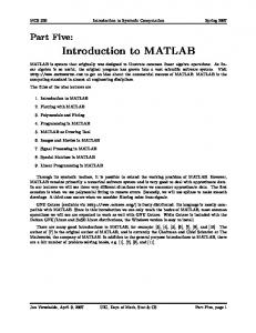
Simulation Example
This exercise is a study of the effect of sample size on the estimates of the coefficient in an OLS regression. The x values for the regression have been generated as uniform random numbers on the interval [0,100). The residuals are simulated standardized normal random variables. The process is repeated for sample sizes of 20, 100 500 and 2500 simulation is repeated 10,000 times. % MATLAB Simulation Example %John C Frain %19 November 2006 % ${ The data files x20.csv, x100.csv, x500.csv and x2500.csv were generated using the code below $} %Generate Data x20 = 100*rand(20,1) save(’x20.csv’,’x20’,’-ASCII’,’-double’) x100 = 100*rand(100,1) save(’x100.csv’,’x100’,’-ASCII’,’-double’) x500 = 100*rand(500,1) save(’x500.csv’,’x500’,’-ASCII’,’-double’) x2500 = 100*rand(200,1) save(’x2500.csv’,’x2500’,’-ASCII’,’-double’) %} clear nsimul=10000; BETA20=zeros(nsimul,1); % vector - results of simulations with 20 obs. x=load(’-ascii’, ’x20.csv’); % load xdata X=[ones(size(x,1),1),x]; % X matrix note upper case X beta = [ 10;2]; % true values of coefficients % for ii = 1 : nsimul; eps = 20.0*randn(size(X,1),1); % simulated error term y = X * beta + eps; % y values 31
betahat = (X’*X)\X’*y; % estimate of beta BETA20(ii,1)=betahat(2); end fprintf(’Mean and st. dev of 20 obs simulation %6.3f %6.3f\n’ ... ,mean(BETA20),std(BETA20)) %hist(BETA,100) BETA100=zeros(nsimul,1); x=load(’-ascii’, ’x100.csv’); % load xdata X=[ones(size(x,1),1),x]; % X matrix note upper case X beta = [ 10;2]; % true values of coefficients % for ii = 1 : nsimul; eps = 20.0*randn(size(X,1),1); % simulated error term y = X * beta + eps; % y values betahat = inv(X’*X)*X’*y; % estimate of beta BETA100(ii,1)=betahat(2); end fprintf(’Mean and st. dev of 100 obs simulation %6.3f %6.3f\n’, ... mean(BETA100),std(BETA100)) BETA500=zeros(nsimul,1); x=load(’-ascii’, ’x500.csv’); % load xdata X=[ones(size(x,1),1),x]; % X matrix note upper case X beta = [ 10;2]; % true values of coefficients % for ii = 1 : nsimul; eps = 20.0*randn(size(X,1),1); % simulated error term y = X * beta + eps; % y values betahat = inv(X’*X)*X’*y; % estimate of beta BETA500(ii,1)=betahat(2); end fprintf(’Mean and st. dev of 500 obs simulation %6.3f %6.3f\n’, ... mean(BETA500),std(BETA500)) BETA2500=zeros(nsimul,1); x=load(’-ascii’, ’x2500.csv’); % load xdata note use of lower case x as vector X=[ones(size(x,1),1),x]; % X matrix note upper case X beta = [ 10;2]; % true values of coefficients % for ii = 1 : nsimul; eps = 20.0*randn(size(X,1),1); % simulated error term
32
y = X * beta + eps; % y values betahat = inv(X’*X)*X’*y; % estimate of beta BETA2500(ii,1)=betahat(2); end fprintf(’Mean and st. dev of 2500 obs simulation %6.3f %6.3f\n’, ... mean(BETA2500),std(BETA2500)) n=hist([BETA20,BETA100,BETA500,BETA2500],1.4:0.01:2.6); plot((1.4:0.01:2.6)’,n/nsimul); h = legend(’Sample 20’,’Sample 100’,’Sample 500’,’Sample 2500’);
The output of this program will look like this. On your screen the graph will display coloured lines. Mean and st. dev of 20 obs simulation 2.000 0.165 Mean and st. dev of 100 obs simulation 2.000 0.065 Mean and st. dev of 500 obs simulation 2.000 0.030 Mean and st. dev of 2500 obs simulation 1.999 0.049 0.14 Sample 20 Sample 100 Sample 500 Sample 2500
0.12
0.1
0.08
0.06
0.04
0.02
0
3 3.1
1.4
1.6
1.8
2
2.2
2.4
2.6
2.8
Data input/output Native MatLab data files
The instruction Save filename saves the contents of the workspace in the file ’filename.mat’. save used in the default manner saves the data in a binary format. The instruction 33
save filename, var1, var2 saves var1 and var2 in the file filename.mat. Similarly the commands Load filename and load filename, var1, var2. load the contents of ’filename.mat’ or the specified variables from the file into the workspace. In general .mat files are nor easily readable in most other packages. They are ideal for use within MATLAB and for exchange between MATLAB users. (note that there may be some incompatibilities between different versions of MATLAB). These .mat files are binary and can not be examined in a text editor. .mat is the default extension for a MATLAB data file. If you use another extension, say .ext the option Save mat filename.ext should be used with the save and load commands. It is possible to use save and load to save and load text files but these instructions are very limited. If your data are in EXCEL or csv format the methods described below are better
3.2
Importing from Excel
The sample file g10xrate.xls contains daily observations on the exchange rates of G10 countries and we wish to analyse them with MATLAB. There are 6237 observations of each exchange rate in the columns of the EXCEL file. The easiest way to import these data into MATLAB is to use the File|import data wizard and follow the prompts. In this case the import wizard did not pick out the series names from the Excel file. I imported the entire data matrix as a matrix and extracted the individual series in MATLAB. One can save the data in MATLAB format for future use in MATLAB This is illustrated in the code below. USXJPN = data(:,1); USXFRA = data(:,2); USXSUI = data(:,3); USXNLD = data(:,4); USXUK = data(:,5); USXBEL = data(:,6); USXGER = data(:,7); USXSWE = data(:,8); USXCAN = data(:,9); USXITA = data(:,10); save(’g10xrate’, ’USXJPN’,’USXFRA’,’USXSUI’,’USXNLD’,’USXUK’,’USXBEL’,’USXGER’, ... ’USXSWE’,’USXCAN’,’USXITA’) Note that I have listed the series to be saved as I did not wish to save the data matrix. The same effect could have been achieved with the uiimport command.
34
3.3
Reading from text files
The import wizard can also import many types of text file including the comma separated files we have used in STATA. The missing data code in Excel csv files is #NA. The version of MATLAB that i am using has problems reading this missing value code and it should be changed to NaN (the MATLAB missing value code) before importing csv data. In this case the import wizard recognised the column names. It is important that you check that all your data has been imported correctly. The MATLAB functions textscan or textread can read various text files and allow a greater degree of flexibility than that available from uiimport. This flexibility is obtained at a cost of greater complexity. Details are given in the Help files. I would think that most users will not need this flexibility but it is there if needed.
3.4
Exporting data to EXCEL, STATA and other programs
The command xlswrite(’filename’,M) writes the matrix M to the file filename in the current working directory. If M is n × m the numeric values in the matrix are written to the first n row and m columns in the first sheet in the spreadsheet. The command csvwrite(’filename’,M) writes the matrix M to the file filename in the current working directory. You can use this file to transfer data to STATA. Alternatively export your Excel file from Excel in csv format.
3.5
Stat/Transfer
Another alternative is to use the Stat/Transfer package which allows the transfer of data files between a large number of statistical packages.
3.6
Formatted Output
The MATLAB function fprintf() may be used to produce formatted output on screen1 . The following MATLAB program gives an example of the us of the fprintf() function.
1 fprintf() is only one of a large number of C-style input/output functions in C. These allow considerable flexibility in sending formatted material to the screen of to a file. The MATLAB help files give details of the facilities available. If further information is required one might consult a standard test book on the C programming language
35
Sample MATLAB program demonstrating Formatted Output clear degrees_c =10:10:100; degrees_f = (degrees_c * 9 /5) + 32; fprintf(’\n\n Conversion from degrees Celsius \n’); fprintf(’ to degrees Fahrenheit\n\n’ ); fprintf(’ Celsius Fahrenheit\n’); for ii = 1:10; fprintf(’%12.2f%12.2f\n’,degrees_c(ii),degrees_f(ii)); end % fprintf(... ’\n\n%5.2f degrees Celsius is equivalent of %5.3f degrees fahrenheit\n’, ... degrees_c(1),degrees_f(1)) Output of Sample MATLAB program demonstrating Formatted Output
Conversion from degrees Celsius to degrees Fahrenheit Celsius
Fahrenheit
10.00 20.00
50.00 68.00
30.00 40.00
86.00 104.00
50.00 60.00
122.00 140.00
70.00 80.00 90.00
158.00 176.00 194.00
100.00
212.00
10.00 degrees Celsius is equivalent of 50.000 degrees fahrenheit Note the following • The first argument of the fprintf() function is a kind of format statement included within ’ marks. • The remaining arguments are a list of variables or items to be printed separated by commas 36
• Within the format string there is text which is produced exactly as set down. There are also statements like %m.nf which produces a decimal number which is allowed m columns of output and has n places of decimals. These are applied in turn to the items in the list to be printed. • This f format is used to output floating point numbers there are a considerable number or other specifiers to output characters, strings, and number in formats other than floating point. • If the list to be printed is too long the formats are recycled. • Not the use of \n which means skip to the next line. This is essential.
3.7
Producing material for inclusion in a paper
A considerable amount of the material in this note was produced from MATLAB mfiles using the —File—Publish to— facilities in the MATLAB m-file editor which produces output in WORD, Powerpoint, LATEX , HTML etc. for inclusion in papers, presentations etc.
4
Decision and Loop Structures.
There are four basic control (Decision or Loop Structures) available in MATLAB if statements The basic form of the if statement is if conditions statements end
The statements are only processed if the conditions are true The conditions can include the following operators
37
== ∼=
equal not equal
< >
less than greater than
=
less than or equal to greater than or equal to
& && |
logical and logical and (for scalars) short-circuiting logical or
|| xor
logical or and (for scalars) short-circuiting logical exclusive or
all any
true if all elements of vector are nonzero true if any element of vector is nonzero
The if statement may be extended if conditions statements1 else statements2 end
in which case statements1 are used if conditions are true and statements2 if false. This if statement may be extended again if conditions1 statements1 elseif conditions2 statements2 else statements3 end
with an obvious meaning (I hope). for The basic form of the for group is for variable = expression statements end Here expression is probably a vector. statements is processed for each of the values in expression. The following example shows the use of a loop within a loop 38
>> for ii = 1:3 for jj=1:3 total=ii+jj; fprintf(’%d + %d = %d \n’,ii,jj,total) end end 1 + 1 = 2 1 + 2 = 3 1 + 3 = 4 2 + 1 = 3 2 + 2 = 4 2 + 3 = 5 3 + 1 = 4 3 + 2 = 5 3 + 3 = 6 while The format of the while statement is while conditions statements end The while statement has the same basic functionality as the for statement. The for statement will be used when one knows precisely when and how many times an operation will be repeated. The statements are repeated so long as conditions are true switch An example of the use of the switch statement follows switch p case 1 x = 24 case 2 x = 19 case 3 x = 15 otherwise error(’p must be 1, 2 or 3’) end Use matrix statements in preference to loops. Not only are they more efficient but they are generally easier to use. That said there are occasions where one can not use a matrix statement.
39
If you wish to fill the elements of a vector or matrix using a loop it is good practice to initial the vector or matrix first. For example if you wish to fill a 100 × 20 matrix, X, using a series of loops one could initialise the matrix using one of the following commands X = ones(100,20) X = zeros(100,20) X = ones(100,20)*NaN X = NaN(100,20)
5
Elementary Plots
Simple graphs can be produced easily in MatLab. The following sequence %values for simulation nsimul=50; beta=[5,1,.1]’; % x1=ones(nsimul,1); %constant x2=[1:nsimul]’; %trend x3=rand(nsimul,1)*2 +3; % Uniform(3,5) x=[x1,x2,x3]; e=randn(nsimul,1)*.2; y= x * beta +e ;
% N(0,.04) %5*x1 + x2 + .1*x3 + e;
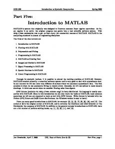
% [nobs,nvar]=size(x); betahat=inv(x’*x)*x’*y %g yhat = x * betahat; % beta(1)*x1-beta(2)*x2-beta(3)*x; resid = y - yhat; plot(x2,resid) title(’Graph Title’) xlabel(’Time’) ylabel(’Residual’)
40
Graph Title 0.5 0.4 0.3 0.2
Residual
0.1 0 −0.1 −0.2 −0.3 −0.4 −0.5
0
10
20
30
40
50
Time repeats the earlier OLS simulation, opens a graph window, draws a graph of the residuals against the trend in the ols-simulation exercise, puts a title on the graph and labels the x and y axes. The vectors x2 and resid must have the same dimensions. This graph was saved in eps format and imported into this document.
6
Systems of Regresssion Equations
This section will show how to use MATLAB to estimate systems of regression equations (Pooled OLS, OLS equation by equation, SOLS (OLS equation by equation),SUR, 2SLS, 3SLS, GMM). The emphasis is on constructing system y (endogenous) X (exogenous) and Z (instrument) matrices which can be used to “jointly” estimate the parameters involved.
7
The LeSage Econometric Toolbox
If you are accustomed to using one of the many packages that deal specifically with econometrics you may think that MATLAB takes a long time to do simple things. It is also clear that many or the more difficult tasks are often easier in MATLAB than in these packages. MATLAB is less of a “‘black box” than many of the other programs.
41
One must really learn and understand the algebra before one can use MATLAB for econometrics. One also knows exactly what one is doing when one has written the routines in MATLAB. The big problem is the lack of elementary econometric facilities in MATLAB. The LeSage MATLAB econometric package adds many of the required functions. It contains about 300 functions, utilities and demonstration programs. A list is included in Appendix A to this note. Full details are available in the toolbox manual which is available at http:// www.spatial-econometrics.com/. The toolbox is designed to produce documentation, example programs, printed and graphical output across a wide range of econometric procedures. Availability on Public Access Computers The toolbox has been added to the MATLAB system on all Public Access computers on the TCD network. The functions are available in the same way as the ordinary MATLAB functions. For example, if y is a n × 1 vector and X is a n × k matrix, the instruction result = ols(y,X) calculates the regression of y on X and various related statistics. The instruction prt_reg(result) produces a summary of the result. Help is available in the command line in MATLAB. Help on the ols function can be found as follows >> help ols PURPOSE: least-squares regression --------------------------------------------------USAGE: results = ols(y,x) where: y = dependent variable vector (nobs x 1) x = independent variables matrix (nobs x nvar) --------------------------------------------------RETURNS: a structure results.meth = ’ols’ results.beta = bhat (nvar x 1) results.tstat = t-stats (nvar x 1) results.bstd = std deviations for bhat (nvar x 1) results.yhat = yhat (nobs x 1) results.resid = residuals (nobs x 1) results.sige
= e’*e/(n-k)
scalar 42
results.rsqr results.rbar results.dw
= rsquared scalar = rbar-squared scalar = Durbin-Watson Statistic
results.nobs results.nvar
= nobs = nvars
results.y results.bint
= y data vector (nobs x 1) = (nvar x 2 ) vector with 95% confidence intervals on beta
--------------------------------------------------SEE ALSO: prt(results), plt(results) --------------------------------------------------Overloaded functions or methods (ones with the same name in other directories) help localmod/ols.m After running the ols function a structure containing the results is available. The variable results.beta contains the estimated β-coefficients, results.tstat their tstatistics, results.bint the 95% confidence intervals for the estimates and similar for the other variables defined. Each estimation command produces its results in a similar structure. To see how to print a summary of these results >> help prt_reg PURPOSE: Prints output using regression results structures --------------------------------------------------USAGE: prt_reg(results,vnames,fid) Where: results = a structure returned by a regression vnames = an optional vector of variable names fid = optional file-id for printing results to a file (defaults to the MATLAB command window) --------------------------------------------------NOTES: e.g. vnames = strvcat(’y’,’const’,’x1’,’x2’); e.g. fid = fopen(’ols.out’,’wr’); use prt_reg(results,[],fid) to print to a file with no vnames -------------------------------------------------RETURNS: nothing, just prints the regression results -------------------------------------------------SEE ALSO: prt, plt --------------------------------------------------Thus to display the results of the previous regression on the screen in MATLAB one would enter2 prt_reg(result) 2 result
in this context is the name of a MATLAB variable and one could substitute for result any valid MATLAB variable name.
43
Availability on other PCs The LeSage toolbox is available for download free on the internet. The only requirement on the package web site is that “Anyone is free to use these routines, no attribution (or blame) need be placed on the author/authors.” The econometrics package is not available by default when MATLAB is installed on a PC. It may be downloaded from http://www.spatial-econometrics.com/. The toolbox is provided as a zipped file which can be unzipped to the MATLAB toolbox directory on your PC ( C:\ProgramFiles\MATLAB704\toolbox or my PC - something similar on yours). This should create a subdirectory econometrics in this toolbox directory This econometrics directory will contain a large number of subdirectories containing the various econometric functions. When you next start MATLAB you can access the functions by adding to the path that MATLAB uses to search for functions. You can do the when you next start MATLAB by —File—Set Path— selecting the Add with subfolders button and navigating to and selecting the econometrics folder. If you select save after entering the directory the functions will be available each time you start MATLAB. If you have the required permissions you can also access the toolbox from the IIS server. The toolbox provides full source code for each function. Thus if no function provides the capabilities that you require it may be possible the amend the function and add the required functionality. If you do such work you should consider submitting you program for inclusion in a future version of the toolbox. By collaborating in this way you are helping to ensure the future of the project The programs in the toolbox are examples of good programming practice and have good comments. If you are starting some serious programming in MATLAB you could learn a lot about programming by reading these programs. Sample run from the LeSage toolbox To illustrate the use of the LeSage toolbox I set out below the output of the demonstration program demo reg.m. This program illustrates many of the various univariate estimation procedures available in the toolbox. % PURPOSE: demo using most all regression functions % % ols,hwhite,nwest,ridge,theil,tsls,logit,probit,tobit,robust %--------------------------------------------------% USAGE: demo_all %--------------------------------------------------clear all; rand(’seed’,10); n = 100; k=3;
44
xtmp = randn(n,k-1); tt = 1:n; ttp = tt’; e = randn(n,1).*ttp; % heteroscedastic error term %e = randn(n,1); b = ones(k,1);
% homoscedastic error term
iota = ones(n,1); x = [iota xtmp]; % generate y-data y = x*b + e; vnames=strvcat(’yvar’,’iota’,’x1’,’x2’); % * * * * * * * reso = ols(y,x);
demo ols regression
prt(reso,vnames); %
* * * * * * *
demo hwhite regression
res = hwhite(y,x); prt(res,vnames); %
* * * * * * *
demo nwest regression
nlag=2; res = nwest(y,x,nlag); prt(res,vnames); %
* * * * * * *
demo ridge regresson
rres = ridge(y,x); prt(rres,vnames); % * * * * * * *
demo logit regression
n = 24; y = zeros(n,1); y(1:14,1) = ones(14,1); % (data from Spector and Mazzeo, 1980) xdata = [21 24 25 26 28 31 33 34 35 37 43 49 ... 51 55 25 29 43 44 46 46 51 55 56 58]; iota = ones(n,1); x = [iota xdata’];
45
vnames=strvcat(’days’,’iota’,’response’); res = logit(y,x); prt(res,vnames); % * * * * * * * n = 32; k=4;
demo probit regression
y = zeros(n,1); % grade variable y(5,1) = 1; y(10,1) = 1; y(14,1) = 1; y(20,1) = 1; y(22,1) = 1; y(25,1) = 1; y(25:27,1) = ones(3,1); y(29,1) = 1; y(30,1) = 1; y(32,1) = 1; x = zeros(n,k); x(1:n,1) = ones(n,1); % intercept x(19:32,2) = ones(n-18,1); % psi variable tuce = [20 22 24 12 21 17 17 21 25 29 20 23 23 25 26 19 ... 25 19 23 25 22 28 14 26 24 27 17 24 21 23 21 19]; x(1:n,3) = tuce’; gpa = [2.66 2.89 3.28 2.92 4.00 2.86 2.76 2.87 3.03 3.92 ... 2.63 3.32 3.57 3.26 3.53 2.74 2.75 2.83 3.12 3.16 ... 2.06 3.62 2.89 3.51 3.54 2.83 3.39 2.67 3.65 4.00 ... 3.10 2.39]; x(1:n,4) = gpa’; vnames=strvcat(’grade’,’iota’,’psi’,’tuce’,’gpa’); resp = probit(y,x); prt(resp,vnames); % results reported in Green (1997, chapter 19) % b = [-7.452, 1.426, 0.052, 1.626 ]
46
% * * * * * * * demo theil-goldberger regression % generate a data set nobs = 100; nvar = 5; beta = ones(nvar,1); beta(1,1) = -2.0; xmat = randn(nobs,nvar-1); x = [ones(nobs,1) xmat]; evec = randn(nobs,1); y = x*beta + evec*10.0; Vnames = strvcat(’y’,’const’,’x1’,’x2’,’x3’,’x4’); % set up prior rvec = [-1.0 1.0
% prior means for the coefficients
2.0 2.0 1.0]; rmat = eye(nvar); bv = 10000.0; % umat1 = loose prior umat1 = eye(nvar)*bv; % initialize prior variance as diffuse for i=1:nvar; umat1(i,i) = 1.0;
% overwrite diffuse priors with informative prior
end; lres = theil(y,x,rvec,rmat,umat1); prt(lres,Vnames); %
* * * * * * *
demo two-stage least-squares regression
nobs = 200;
47
x1 = randn(nobs,1); x2 = randn(nobs,1); b1 = 1.0; b2 = 1.0; iota = ones(nobs,1); y1 = zeros(nobs,1); y2 = zeros(nobs,1); evec = randn(nobs,1); % create simultaneously determined variables y1,y2 for i=1:nobs; y1(i,1) = iota(i,1)*1.0 + x1(i,1)*b1 + evec(i,1); y2(i,1) = iota(i,1)*1.0 + y1(i,1)*1.0 + x2(i,1)*b2 + evec(i,1); end; vname2 = [’y2-eqn ’, ’y1 var ’, ’constant’, ’x2 var
’];
% use all exogenous in the system as instruments xall = [iota x1 x2]; % do tsls regression result2 = tsls(y2,y1,[iota x2],xall); prt(result2,vname2);
% * * * * * * * demo robust regression % generate data with 2 outliers nobs = 100; nvar = 3; vnames = strvcat(’y-variable’,’constant’,’x1’,’x2’); x = randn(nobs,nvar); x(:,1) = ones(nobs,1); beta = ones(nvar,1);
48
evec = randn(nobs,1); y = x*beta + evec; % put in 2 outliers y(75,1) = 10.0; y(90,1) = -10.0; % get weighting parameter from OLS % (of course you’re free to do differently) reso = ols(y,x); sige = reso.sige; % set up storage for bhat results bsave = zeros(nvar,5); bsave(:,1) = ones(nvar,1); % loop over all methods producing estimates for i=1:4; wfunc = i; wparm = 2*sige; % set weight to 2 sigma res = robust(y,x,wfunc,wparm); bsave(:,i+1) = res.beta; end; % column and row-names for mprint function in.cnames = strvcat(’Truth’,’Huber t’,’Ramsay’,’Andrews’,’Tukey’); in.rnames = strvcat(’Parameter’,’constant’,’b1’,’b2’); fprintf(1,’Comparison of alternative robust estimators \n’); mprint(bsave,in); res = robust(y,x,4,2); prt(res,vnames); %
* * * * * * *
demo regresson with t-distributed errors
res = olst(y,x); prt(res,vnames);
49
% * * * * * * * res = lad(y,x); prt(res,vnames);
demo lad regression
% * * * * * * * demo tobit regression n=100; k=5; x = randn(n,k); x(:,1) = ones(n,1); beta = ones(k,1)*0.5; y = x*beta + randn(n,1); % now censor the data for i=1:n if y(i,1) < 0 y(i,1) = 0.0; end; end; resp = tobit(y,x); vnames = [’y
’,
’iota ’, ’x1var ’, ’x2var ’, ’x3var ’, ’x4var ’]; prt(resp,vnames);
% * * * * * * * demo thsls regression clear all; nobs = 100; neqs = 3; x1 = randn(nobs,1); x2 = randn(nobs,1); x3 = randn(nobs,1); b1 = 1.0; b2 = 1.0;
50
b3 = 1.0; iota = ones(nobs,1); y1 = zeros(nobs,1); y2 = zeros(nobs,1); y3 = zeros(nobs,1); evec = randn(nobs,3); evec(:,2) = evec(:,3) + randn(nobs,1); % create cross-eqs corr % create simultaneously determined variables y1,y2 for i=1:nobs; y1(i,1) = iota(i,1)*10.0 + x1(i,1)*b1 + evec(i,1); y2(i,1) = iota(i,1)*10.0 + y1(i,1)*1.0 + x2(i,1)*b2 + evec(i,2); y3(i,1) = iota(i,1)*10.0 + y2(i,1)*1.0 + x2(i,1)*b2 + x3(i,1)*b3 + evec(i,3); end;
vname1 = [’y1-LHS ’, ’constant’, ’x1 var vname2 = [’y2-LHS ’y1 var
’]; ’, ’,
’constant’, ’x2 var ’]; vname3 = [’y3-LHS ’y2 var
’, ’,
’constant’, ’x2 var ’, ’x3 var
’];
% set up a structure for y containing y’s for each eqn y(1).eq = y1; y(2).eq = y2; y(3).eq = y3; % set up a structure for Y (RHS endogenous) for each eqn Y(1).eq = []; Y(2).eq = [y1]; Y(3).eq = [y2];
51
% set up a structure fo X (exogenous) in each eqn X(1).eq = [iota x1]; X(2).eq = [iota x2]; X(3).eq = [iota x2 x3]; % do thsls regression result = thsls(neqs,y,Y,X); vname = [vname1 vname2 vname3]; prt(result,vname); % * * * * * * * demo olsc, olsar1 regression % generate a model with 1st order serial correlation n = 200; k = 3; tt = 1:n; evec = randn(n,1); xmat = randn(n,k); xmat(:,1) = ones(n,1); beta = ones(k,1); beta(1,1) = 10.0; % constant term y = zeros(n,1); u = zeros(n,1); for i=2:n; u(i,1) = 0.4*u(i-1,1) + evec(i,1); y(i,1) = xmat(i,:)*beta + u(i,1); end; % truncate 1st 100 observations for startup yt = y(101:n,1); xt = xmat(101:n,:); n = n-100; % reset n to reflect truncation Vnames = [’y
’,
’cterm’,
52
’x2 ’x3
’, ’];
% do Cochrane-Orcutt ar1 regression result = olsc(yt,xt); prt(result,Vnames); % do maximum likelihood ar1 regression result2 = olsar1(yt,xt); prt(result2,Vnames);
% * * * * * * * demo switch_em, hmarkov_em regressions clear all; % generate data from switching regression model nobs = 100; n1 = 3; n2 = 3; n3 = 3; b1 = ones(n1,1); b2 = ones(n2,1)*5; b3 = ones(n3,1); sig1 = 1; sig2 = 1; randn(’seed’,201010); x1 = randn(nobs,n1); x2 = randn(nobs,n2); x3 = randn(nobs,n3); ytruth = zeros(nobs,1); for i=1:nobs; if x3(i,:)*b3