Social and Personality Psychology Compass 2/2 (2008): 842–860, 10.1111/j.1751-9004.2007.00059.x
An Introduction to Multilevel Modeling for Social and Personality Psychology John B. Nezlek* College of William & Mary
Abstract
Multilevel modeling is a technique that has numerous potential applications for social and personality psychology. To help realize this potential, this article provides an introduction to multilevel modeling with an emphasis on some of its applications in social and personality psychology. This introduction includes a description of multilevel modeling, a rationale for this technique, and a discussion of applications of multilevel modeling in social and personality psychological research. Some of the subtleties of setting up multilevel analyses and interpreting results are presented, and software options are discussed.
Once you know that hierarchies exist, you see them everywhere. (Kreft and de Leeuw, 1998, 1)
Whether by design or nature, research in personality and social psychology and related disciplines such as organizational behavior increasingly involves what are often referred to as multilevel data. Sometimes, such data sets are referred to as ‘nested’ or ‘hierarchically nested’ because observations (also referred to as units of analysis) at one level of analysis are nested within observations at another level. For example, in a study of classrooms or work groups, individuals are considered to be nested within groups. Similarly, in diary-style studies, observations (e.g., diary entries) are nested within persons. What is particularly important for present purposes is that when you have multilevel data, you need to analyze them using techniques that take into account this nesting. As discussed below (and in numerous places, including Nezlek, 2001), the results of analyses of multilevel data that do not take into account the multilevel nature of the data may (or perhaps will) be inaccurate. This article is intended to acquaint readers with the basics of multilevel modeling. For researchers, it is intended to provide a basis for further study. I think that a lack of understanding of how to think in terms of hierarchies and a lack of understanding of how to analyze such data inhibits researchers from applying the ‘multilevel perspective’ to their work. For those simply interested in understanding what multilevel © 2008 The Author Journal Compilation © 2008 Blackwell Publishing Ltd
Multilevel Analyses
843
modeling is and how to interpret the results of such analyses, it should help them understand what was done and why it was done as they encounter multilevel analyses in their scholarly activities. This article describes the multilevel perspective as it pertains to the types of research social and personality psychologists frequently conduct. This description includes some of the types of data that can be conceptualized within a multilevel framework and some basic principles underlying the analyses of multilevel data. This article is intended as an introduction to multilevel modeling, and as such, it only touches the surface of various topics. Readers who are interested in the details of multilevel modeling should consult any of the following, all of which are intended as introductions: Raudenbush and Bryk (2002), Snijders and Boskers (1999), and Kreft and de Leeuw (1998). Readers interested in the application of multilevel modeling to specific research designs may want to consult papers mentioned in the section on potential applications. The Importance of Understanding Levels of Analysis Multilevel analyses are appropriate when data have been collected at multiple levels simultaneously. In this instance, ‘levels’ refers to how the data are organized, and more important statistically, to whether observations are dependent (or not independent), a topic discussed below. The traditional (and recommended) way to refer to these levels is by number (level 1, level 2, etc.), with larger numbers indicating levels that are higher in the hierarchy.1 For example, in a study in which persons are organized in groups (e.g., work groups), measures describing individuals (e.g., productivity) would constitute the level 1 data, and measures describing the groups (e.g., position in an organization) would constitute the level 2 data. Studies in which multiple observations are taken from individuals (e.g., a diary study) can also be thought of as multilevel data, with observations (e.g., daily diary entries) constituting the level 1 data and individual characteristics (e.g., personality traits) constituting the level 2 data. One of the important characteristics of such data is that the level 1 observations are not independent. People in a group share whatever characteristics the group has, and the diary entries people provide have in common the characteristics of the person. This lack of independence means that traditional ordinary least-squares (OLS) techniques such as multiple regression in which level 1 observations are treated as independent observations cannot be used because such analyses violate a fundamental assumption – the independence of observations. For example, in a study of groups, it is fundamentally wrong to conduct a single level regression analysis in which group level measures are assigned to the individual members of groups and are then used in the analysis as if they were individual level measures. Similarly, in a diary-style study, it is fundamentally wrong to conduct an analysis in which daily observations are the units of © 2008 The Author Social and Personality Psychology Compass 2/2 (2008): 842–860, 10.1111/j.1751-9004.2007.00059.x Journal Compilation © 2008 Blackwell Publishing Ltd
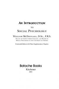
844 Multilevel Analyses Table 1 Differences across groups in within-group relationships Group 1
Group 2
Group 3
X
y
x
y
x
y
1 2 3 4 5 3
8 7 6 5 4 6
4 5 6 7 8 6
13 12 11 10 9 11
9 10 11 12 13 11
18 17 16 15 14 16
analysis (i.e., data entries) and individual (person level) measures such as personality characteristics are assigned to each day a person maintained a diary and then used as if they were daily level measures. In both cases, the observations are not independent. In addition to violating the independence assumption (which by itself is sufficient to render them flawed), single-level analyses that ignore the hierarchical structure of the data can provide misleading results. For example, assume a data set in which there are three groups with five persons in each group, and each person provides two measures, x and y (see Table 1). If the data in Table 1 were analyzed by treating the observations as 15 independent observations, the correlation between the two measures would be 0.73. It is clear from looking at the data, however, that the relationship within each group is negative, making suspect any procedure that estimates a positive relationship. Some have argued that such problems can be solved by using a variable indicating group membership, what is sometimes referred to as ‘least squares dummy-codes’ analysis. Including such terms can reduce the influence on results of mean differences between level 2 units of analysis, although such analyses still assume that relationships between variables are constant across groups. The possibility that level 1 (e.g., within-group) relationships vary between level 2 units of analysis (e.g., groups) can be examined by including interaction terms between such dummy codes and level 1 variables; however, even when such dummy codes are included, the analyses violate important assumptions about sampling error. See Nezlek (2001) for a discussion of the shortcomings of various types of OLS analyses of multilevel data. Illustrative Applications As Kreft and de Leeuw (1998) noted, understanding what hierarchies are often leads researchers to recognize the hierarchical nature of data they have collected or are considering collecting. Before describing multilevel © 2008 The Author Social and Personality Psychology Compass 2/2 (2008): 842–860, 10.1111/j.1751-9004.2007.00059.x Journal Compilation © 2008 Blackwell Publishing Ltd
Multilevel Analyses
845
modeling analyses per se, I will describe applications of multilevel modeling to help readers think about how multilevel modeling might be applied to their specific interests. Note that these descriptions are meant to be illustrative, not exhaustive. Within contemporary social and personality psychology, perhaps the most common use of multilevel modeling is the analysis of various types of diary data. A discussed by Wheeler and Reis (1991), diary-style studies (including what are sometimes referred to as intensive repeated measures or experience sampling designs) can be categorized in terms of the basis on which data are collected. In interval-contingent studies, data are collected at certain intervals, which may be fixed (e.g., end-of-day studies) or random (e.g., ‘beeper’ studies). In event-contingent studies, data are collected whenever a certain type of event occurs. Social interaction diary studies, frequently relying on some variant of the Rochester Interaction Record (Wheeler & Nezlek, 1977), are examples of event-contingent data structures. In both cases, individual observations (diary entries, social interactions, etc.) can be thought of as level 1 observations that are nested within persons (level 2 observations). See Nezlek (2001) for a general discussion of multilevel modeling analyses of such data and Nezlek (2003) for a more specific discussion of multilevel analyses of social interaction diary data. Multilevel modeling may also be appropriate for personality psychologists who are interested in within-person variability in psychological states (e.g., Fleeson, 2001). In such studies, state level observations are nested within persons. See Nezlek (2007a, 2007b) for discussions of multilevel analyses of such data structures. The analyses of data collected in groups also calls for multilevel modeling. In studies in which participants are in groups, individuals are the level 1 observations and groups are the level 2 observations (i.e., persons are nested within groups). See Nezlek and Zyzniewski (1998) for an introduction to using multilevel modeling to analyze data collected in groups, and see Kenny, Mannetti, Pierro, Livi, and Kashy (2002) for a more detailed discussion of this topic. The use of multilevel modeling in cross-cultural studies, which often concern topics of interest to social and personality psychologists, is increasing. In cross-cultural research, samples can be collected in different countries, and in such studies, persons can be treated as nested within countries, and for such cross-cultural studies, some considerations may be more important than they are for other types of multilevel designs. For example, differences in sample sizes may not correspond to differences in populations, and depending upon the target of inference, in such cases, analysts may want to conduct some type of weighted analysis that takes into account differences in the populations of each country. Given the difficulties inherent in collecting data in multiple countries, researchers might be able to collect data in only a few countries. In such cases, it might be difficult to conduct the types of multilevel analyses described in © 2008 The Author Social and Personality Psychology Compass 2/2 (2008): 842–860, 10.1111/j.1751-9004.2007.00059.x Journal Compilation © 2008 Blackwell Publishing Ltd
846 Multilevel Analyses
this article, a topic discussed below. See Nezlek (forthcoming) for a more detailed discussion of the use of multilevel modeling in cross-cultural research. Using multilevel modeling to analyze data in which participants respond to different stimuli is relatively underutilized. Just as we can consider the days of a diary as nested within persons, responses to a series of stimuli (e.g., ratings of 30 situations) can be considered as nested within persons. In such cases, the types of techniques discussed in this article can be used to estimate within-person relationships among ratings, and the estimates provided by these techniques will be more accurate than estimates provided by other means such as within-person correlations or regression coefficients. Moreover, the present techniques provide better estimates than comparable OLS techniques of between-person differences in such within-person relationships. Along these lines, multilevel analyses can be used to analyze reaction time data collected in experiments, and interested readers should consult Richter (2006) for an excellent discussion of such applications. Sampling Error within Multilevel Data Structures In a multilevel data structure, units of observations are randomly sampled from populations at different levels simultaneously. For example, in a study of group decision-making, individual participants are sampled to provide a basis for making inferences about people. At the same time, the groups that are formed are meant to provide a basis for making inferences about groups. Similarly, in a diary-style study, days in a person’s life are sampled to provide a basis for making inferences about each person, and persons are sampled to provide a basis for making inferences about people. What is significant about such multiple sampling is that the error associated with sampling at each level of analysis needs to be estimated. If the people involved in a group process study were used to form different groups, the relationships that were found would probably be similar to, but not the same as the relationships found in the first sampling. Similarly, the within-person relationships found in a sample of days from a person’s life would probably be similar to, but not exactly the same as, the relationships found in another sample of days. In both the group process and diary study, there are two sources of sampling error. The need to take into account simultaneously the sampling error at each level of analysis is why it is not appropriate to use a series of OLS analyses to estimate within-group (or within-person) relationships and then use such coefficients in other analyses. For example, it is not appropriate to calculate measures of within-group processes and then use these measures in a group-level analysis. Similarly, it is not appropriate to calculate withinperson measures such as correlations or regression coefficients and then use such measures in person level analyses. Such ‘two-stage’ least-squares © 2008 The Author Social and Personality Psychology Compass 2/2 (2008): 842–860, 10.1111/j.1751-9004.2007.00059.x Journal Compilation © 2008 Blackwell Publishing Ltd
Multilevel Analyses
847
techniques (even what are sometimes called weighted least squares) do not provide estimates of relationships that are as accurate as those provided by the random coefficient techniques discussed in this article. This is due in part to the fact that with two-stage least-squares and similar techniques, the errors at the two levels of analysis are necessarily separate. Multilevel random coefficient modeling relies on maximum likelihood algorithms that allow for the simultaneous estimation of multiple unknowns (i.e., error terms). The techniques described in this article provide numerous advantages over comparable OLS techniques, and these advantages are pronounced under two conditions. First, when hypotheses of interest concern withinunit relationships (e.g., within-group relationships in a group study, within-person relationships in a diary study, etc.). Second, when the data structure is irregular (e.g., when groups differ in size, when people provide different numbers of diary entries, etc.). These advantages are the result of the specific statistical techniques that should be used to analyze multilevel data, and this is discussed in some detail in Nezlek (2001). What Is Multilevel Modeling? The present discussion of multilevel modeling concerns what is technically referred to as ‘multilevel random coefficient modeling’ (MRCM). The term ‘random’ reflects the fact the technique models (or estimates) random coefficients, something discussed below. Multilevel modeling is relatively straightforward conceptually. For each level 2 unit (e.g., a group in group studies, a person in diary studies), a level 1 (e.g., within-group or within-person) model is estimated. Such models are functionally equivalent to a standard OLS regression. For example, in a study of groups, the dependent measure might be productivity and the independent measures (predictors) could be motivation, personality, etc. For each group, a model (a regression equation with coefficients) is estimated describing the relationships among these variables. These coefficients then become the dependent measures at the next level of analysis. This last sentence describes the heart of the matter – relationships (or coefficients describing relationships), not only means, become dependent measures.2 The simplest model is what is usually called a ‘totally unconditional’ or ‘null’ model – there are no predictors at either level of analysis. The equations for such a model are below. In standard MRCM nomenclature, level 1 coefficients are referred to as βs, (subscripted 0 for the intercept, 1 for the first coefficient, 2 for the second, etc.), and the basic level 1 model is: yij = β0j + rij © 2008 The Author Social and Personality Psychology Compass 2/2 (2008): 842–860, 10.1111/j.1751-9004.2007.00059.x Journal Compilation © 2008 Blackwell Publishing Ltd
848 Multilevel Analyses
In this model, there are ‘i’ level 1 observations nested within ‘j’ level 2 units of a continuous variable y that are modeled as a function of the intercept for each level 2 unit (β0j, the mean of y) and error (rij), and the variance of rij is the level 1 random variance. Level 1 coefficients are then modeled (analyzed) at level 2, and level 2 coefficients are referred to as γs. There is a separate level 2 equation for each level 1 coefficient. The basic level 2 model is: β0j = γ00 + u0j In this model, the mean of y for each of j units of analysis (β0j) is modeled as a function of the grand mean (γ00) and error (u0j), and the variance of u0j is the level 2 variance. Such models are referred to as unconditional at level 2 because β0j is not modeled as a function of another variable at level 2. In other words, no hypotheses (other than testing if the mean, γ00, is significantly different from 0) are tested. Although such unconditional models do not test hypotheses per se, they are useful first steps because they provide estimates of the level 1 and 2 variances (the variances of rij and u0j). Such estimates may indicate where further analyses would be informative (i.e., ‘where the action is’ in a data set). Hypotheses are tested by adding variables at either or both levels of analysis. For example, if a researcher wanted to know if group productivity was related to how long a group had been together, the following model could be examined: yij = β0j + rij β0j = γ00 + γ01(Time) + u0j In this analysis, y would be an individual-level measure of productivity (e.g., how many widgets a worker produced), β0j would be mean productivity (for j groups), and the hypothesis would be tested via the significance of the γ01 coefficient at level 2. If γ01 was positive and significantly different from 0, then we could conclude that there was a positive relationship between productivity and the time a group had been together. If γ01 was significant and negative, the relationship would be negative, and so forth. Those unfamiliar with MRCM might ask: ‘Why not simply calculate a mean for each group and then use these means in a group level analysis?’ Although the question is reasonable, the answer is clear – MRCM provides better estimates of group means than the simple average. This superiority is due to the fact that in MRCM, the coefficients describing a group are weighted by the reliability of the scores (how consistent the scores are in a group) and by the number of observations in the group – something called ‘precision weighting’. Not all means are created equal. The mean of 9, 9, 9 and 1, 1, 1 is 5. The mean of 4, 4, 4 and 6, 6, 6 is also 5. The second 5 is a ‘better’ 5 (i.e., more representative) than the first 5. MRCM takes such differences into account. © 2008 The Author Social and Personality Psychology Compass 2/2 (2008): 842–860, 10.1111/j.1751-9004.2007.00059.x Journal Compilation © 2008 Blackwell Publishing Ltd
Multilevel Analyses
849
Nevertheless, the advantages of MRCM over OLS-based analyses are even more pronounced when hypotheses of interest concern within-unit relationships. For example, assume a cross-cultural study in which measures of political conservatism and independent self-construal have been collected in numerous countries, and the hypothesis of interest concerns the within-country relationship between these two measures. Within a multilevel framework, such a hypothesis would be tested with the following model: yij = β0j + β1j(Self-construal) + rij β0j = γ00 + u0j β1j = γ10 + u1j In the level 1 model, the relationship between conservatism and selfconstrual is represented by the β1j coefficient (called a slope to distinguish it from an intercept), and a slope would be estimated for each of j countries. The hypothesis is tested at level 2 by the significance of the γ10 coefficient – is the mean slope significantly different from 0? Such an analysis is much more accurate than a comparable OLS analysis such as calculating a correlation for each country, converting them using a r to Z transform, and then doing a t-test of the mean correlation coefficient. As discussed in Nezlek (2001), there are various reasons for this, mostly having to do with how MRCM incorporates into the estimates of coefficients the unreliability of the covariances underlying the coefficients. By extension, MRCM also excels (compared with OLS techniques) when hypotheses of interest concern how slopes vary across level 2 units of analysis. For example, does the relationship between conservatism and self-construal vary as a function of industrialization as measured by gross domestic product (GDP)? Such a hypothesis would be tested at level 2 with the following model: β0j = γ00 + γ01(GDP) + u0j β1j = γ10 + γ11(GDP) + u1j The possibility that the conservatism–construal slope varies as a function of GDP is tested by the γ11 coefficient. This is sometimes called a ‘crosslevel interaction’ (because a level 1 relationship varies as a function of level 2 variable) or a ‘slopes as outcomes’ analysis (because a slope from level 1 becomes the outcome or dependent measure at level 2). As discussed below, interpreting such results is best done by generating predicted or estimated values (e.g., estimating conservatism-construal slopes for countries that are ±1 SD on GDP). Note that GDP is also included in the equation for the intercept. The norm in MRCM is to include, at least in initial models, the same level 2 predictors for all coefficients. © 2008 The Author Social and Personality Psychology Compass 2/2 (2008): 842–860, 10.1111/j.1751-9004.2007.00059.x Journal Compilation © 2008 Blackwell Publishing Ltd
850 Multilevel Analyses
Non-linear and Categorical Outcomes The preceding discussion has focused on continuous outcomes (e.g., scores on scales or instruments) in part because for most researchers, most of their dependent measures will probably be continuous. Nevertheless, many outcomes of interest may be categorical (pass-fail, accepted-rejected, etc.) or non-linearly distributed. Such outcomes violate an important assumption underlying multilevel (and single level OLS) analyses – the independence of the mean and the variance. For example, the variance of a binomial outcome is npq, where n is the number of observations, p is the probability, and q = 1 – p. Analyzing such data requires the use of specific techniques that eliminate this dependence (and other problems). The specific ways in which the analyses of non-linear and categorical outcomes deal with violations of assumptions varies depending upon the nature of the outcome, and a discussion of these differences is well beyond the scope of this paper. Interested readers should consult a text on multilevel modeling such as Snijders and Boskers (1999) or Raudenbush and Bryk (2002) for more details. Centering Centering refers to the reference value used to estimate an intercept. For OLS regression, this reference value is invariably the sample mean. The intercept represents the expected value for an observation that is at the mean on all the predictors in a model. In MRCM, there are other options. At level 1, predictors can be uncentered (the intercept represents the expected value for an observation with a score of 0 on a predictor), group-mean centered (the intercept represents the expected value for an observation with a score at the mean for its groups), or grand-mean centered (the intercept represents the expected value for an observation with a score at the grand mean). At level 2, predictors can be either uncentered or grand-mean centered. Broadly speaking, centering at level 1 tends to influence parameter estimates more than centering at level 2 in part because centering at level 1 changes the meaning of the intercept and can change the error structure. In terms of selecting different options, group-mean centering at level 1 eliminates level 2 differences in predictors, whereas grand-mean centering at level 1 introduces level 2 differences into the estimates of level 1 parameters. Using the previous example of conservatism and self-construal, if self-construal is group-mean centered, differences across countries in self-construal do not influence parameter estimates. This is the closest (conceptually) to conducting a regression analysis for each country and then analyzing these coefficients in another analysis. If self-construal is entered grand-mean centered, then whatever differences exist between countries in self-construal will influence the parameter estimates (e.g., slopes or within-country relationships). © 2008 The Author Social and Personality Psychology Compass 2/2 (2008): 842–860, 10.1111/j.1751-9004.2007.00059.x Journal Compilation © 2008 Blackwell Publishing Ltd
Multilevel Analyses
851
As discussed by Nezlek (2001) and Raudenbush and Bryk (2002), choices about centering should reflect substantive issues – what does the analyst want the intercept to represent and why? Blanket recommendations to center one way or another should be ignored because no single rule can cover all cases. Unfortunately, space limitations do not permit detailed consideration in this article of centering options in MRCM, and interested readers should consult Enders and Tofighi (2007) for a detailed discussion of centering options and should consult basic multilevel texts for advice regarding this issue. Random Error and Specifying Error Structures For analysts whose primary training has concerned OLS analyses such as single-level regression, there can be some confusion regarding the definition of random variation. In OLS analyses, there is only one variance estimate, which is referred to as error, residual, or random variation. In contrast, in MRCM, the variance of any parameter is divided into true variance and random variance, and each coefficient can have its own random error term. Moreover, tests of significance of the fixed coefficients are based on true variance, not random variance. In MRCM, coefficients can be estimated in three ways: (i) randomly varying, if an accompanying random error term is estimated; (ii) fixed, if no accompanying random error term is estimated; and (iii) non-randomly varying, if no accompanying random error term is estimated, but differences in the coefficient are modeled with a variable at the next level. In the previous cross-cultural example, if the coefficient representing the withincountry relationship between conservatism and self-construal (β1j) was modeled without a random error term (i.e., the u1jt term was dropped), it would be described as a fixed coefficient. If the random term was included, it would be described as a random coefficient. Random error terms are tested for significance, and the result of this test indicates if there is enough information to separate true and random error. Multilevel modelers typically recommend using a more liberal significance level for such tests (at least 0.10) because in most instances, coefficients are theoretically or conceptually random, and to the extent that it is possible, the model should reflect this. Nonetheless, when a random error term is obviously not significant (e.g., p > 0.20), most modelers recommend dropping the term – there is no need to use the information in the data to estimate something that cannot be estimated. Some interpret the absence of a random error term to mean that a coefficient does not vary. This is not really the case. Without a random error term, the model is not estimating the random variability of a coefficient; however, non-random variability in a coefficient can still be examined. For the cross-cultural example, GDP could be included in the © 2008 The Author Social and Personality Psychology Compass 2/2 (2008): 842–860, 10.1111/j.1751-9004.2007.00059.x Journal Compilation © 2008 Blackwell Publishing Ltd
852 Multilevel Analyses
level 2 equation for the level 1 conservatism-construal slope regardless of whether the error term was estimated. When a level 2 variable is used to predict a level 1 coefficient that has been fixed, the level 1 coefficient is described as being modeled as ‘non-randomly varying’. Although the error structure for a model rarely tests hypotheses per se, the error structure needs to be properly specified before conducting tests of the fixed effects because including or excluding random error terms can affect the results of significance tests of the fixed effects. More detailed discussion of specifying error structures in multilevel models can be found in Nezlek (2001) and in any introductory multilevel modeling text. Model Building Although there are no true, hard, and fast rules about how to build a model in MRCM (i.e., how to add terms, specify error structures, etc.), there are some widely accepted guidelines. First, most multilevel modelers recommend finalizing (or building) level 1 models before adding terms at level 2. For example, in a study of decision-making in groups in which persons are nested within groups, individual differences such as measures of personality should be included at level 1 before examining how relationships (slopes) between such individual differences, and decisions vary as a function of group characteristics. The ‘final’ level 1 model should include predictors of interest and should specify whether the coefficients representing these predictors are modeled as random or fixed (i.e., the error structure needs to be specified). Second, there is broad agreement among multilevel modelers that analysts should use forward, rather than backward-stepping, procedures, particularly when building level 1 models. When using forward stepping, individual variables are added to a model and checked for significance, and if the coefficient for an individual variable is not significant, the variable is deleted. When using backward stepping, all variables of interest are added simultaneously at the beginning, and a variable is eliminated if the accompanying coefficient is not significant. Forward stepping is recommended over backward stepping for MRCM because of the number of parameters that need to be estimated when a variable is included. For example, assume a level 1 model with a single predictor. In such a model, five parameters are estimated: (i) the fixed and random terms for the intercept; (ii) the fixed and random terms for the slope; and (iii) the covariance between the two random error terms. If a second predictor is added, nine parameters are estimated: a fixed a random term for the intercept and the two predictors (n = 6) and the covariances among the three random terms (n = 3). If a third predictor is added, 14 parameters are estimated: a fixed and random term for the intercept and the three predictors (n = 8) and the covariances among the four random © 2008 The Author Social and Personality Psychology Compass 2/2 (2008): 842–860, 10.1111/j.1751-9004.2007.00059.x Journal Compilation © 2008 Blackwell Publishing Ltd
Multilevel Analyses
853
terms (n = 6). As variables and parameters are added, models may begin to tax what is sometimes called the ‘carrying capacity’ of a data set – the number of parameters a data set can estimate. Analysts who are accustomed to including all their variables in a single analyses (the ‘Soldier of Fortune’ philosophy: ‘Kill ‘em all and let God sort them out’) will need to either gather large data sets that provide a basis for including large numbers of predictors simultaneously, or they will need to build their models more carefully. The norm among many multilevel modelers is to build tight, parsimonious models that include only those variables that have explanatory power rather than larger models that will provide less precise estimates for a large number of variables that may vary considerably in importance and explanatory power. Interpreting and Reporting Results The results of a MRCM analyses can be bewildering, particularly when using a program that was not designed specifically to conduct MRCM (see section on software below). Nevertheless, the following will help researchers navigate the numerical jungle regardless of the program that has created it. 1. For almost all purposes, analysts should focus on tests of fixed coefficients (sometimes called fixed effects); for example, is a slope significantly different from 0. Almost all hypotheses will concern fixed coefficients of one sort or another. Frequently, analysts over-interpret random error terms, particularly non-significant random terms. Frequently, researchers claim that a coefficient is constant (does not vary) across units of analysis because the random error term associated with that coefficient is not significant. It is important to note that although the absence of a significant random error term is consistent with the hypothesis that a coefficient does not vary, it cannot prove such a hypothesis. Moreover, as noted above, coefficients can vary non-randomly. Simply because a random error term is not estimated for a coefficient (which some would take to mean that there is no variability in the coefficient) does not mean that variability in that coefficient cannot be analyzed. 2. To interpret and report results, many multilevel modelers recommend estimating predicted values. For example, assume that a level 2 variable moderates a level 1 slope (i.e., a relationship between two level 1 variables varies as a function of a level 2 variable). If the level 2 variable is categorical, estimated slopes for each category or groups can be estimated. If the level 2 variable is continuous, estimated slopes for specific values of the level 2 variables (e.g., ±1 SD) can be estimated. 3. All coefficients estimated in a MRCM analysis are unstandardized. Attempting to standardize coefficients (e.g., dividing a fixed effect by some type of error term) is risky at best. Analysts who are concerned © 2008 The Author Social and Personality Psychology Compass 2/2 (2008): 842–860, 10.1111/j.1751-9004.2007.00059.x Journal Compilation © 2008 Blackwell Publishing Ltd
854 Multilevel Analyses
about the effect of differing variances on their analyses or who want some type of standardized metric should transform their data before analysis. 4. Estimating effect sizes based on variances estimates within the multilevel context is a bit complex, particularly compared with OLS analyses (see Raudenbush & Bryk, 2002, for an informed discussion). In fact, some multilevel modelers (e.g., Kreft & deLeeuw, 1998, p. 119) recommend avoiding altogether the use of variance estimates to describe effect sizes. Part of this difficulty stems from the fact that residual variance estimates and significance tests of individual coefficients are estimated separately within MRCM, whereas within OLS analyses, significance tests are based upon reductions in residual variances. Within OLS regression, the F-ratio for a variable that is added to a model is directly related to changes in residual variance. Within MRCM, it is possible to add a significant predictor to a model with either no change (or even an increase) in residual variance, something that is not possible in OLS. Within this context, the following guidelines may be helpful. Similar to OLS, effect sizes can be estimated by estimating the reduction in residual variance resulting from the inclusion of predictors. My experience is that adding a single predictor and comparing the residual variance to the residual variance from a model with no predictors seems to produce fairly reliable estimates. It also seems that the problems described above are more pronounced at level 1 than at level 2. Finally, some editors will insist that authors provide effect size estimates regardless of (or without a knowledge of ) these problems. In such cases, authors may want to report such estimates with a simple caveat that they may not be totally accurate. Design Considerations The preceding has focused on conducting and describing the results of multilevel modeling analyses. When planning a study (or evaluating an existing study), other considerations can be important, and I will briefly discuss two of these: the number of levels that should be used and sample size and power. In most cases, the levels needed for an analysis will be suggested rather straightforwardly by the data. For example, two level models would be appropriate when students are nested within classrooms or days of a diary are nested within persons. Sometimes, however, an additional level of nesting may need to be considered. Should classrooms be nested within schools? If data are collected on multiple occasions each day, should occasions be nested within days and days nested within persons? Such questions can be answered in various ways. First and foremost, are there enough observations to constitute a level of analysis? Only two © 2008 The Author Social and Personality Psychology Compass 2/2 (2008): 842–860, 10.1111/j.1751-9004.2007.00059.x Journal Compilation © 2008 Blackwell Publishing Ltd
Multilevel Analyses
855
schools or only two occasions of measurement per day do not provide a good basis for estimating between-school or within-day parameters. Second, and related, can the data estimate random effects at all levels of analysis? If not, perhaps an additional level of analysis stretches the data too thinly. Sometimes, one type of nesting or another might seem appropriate (e.g., students within classes or within schools). In such cases, analysts need to determine what the psychologically meaningful hierarchy is, something that may be suggested previous research. A related question is power: How many observations are needed at each level of analysis? Unfortunately, estimating power for multilevel designs is considerably more complicated than estimating power for single level analyses. In a multilevel design, power depends on the number of observations at each level of analysis, the variance distributions of measures, the type of effect being examined (e.g., within levels or cross-levels), to mention a few. Such complexity makes it impossible to provide hard and fast rules. Nevertheless, some guidance is available, and two good sources for advice are Maas and Hox (2005) and Richter (2006). Software Options The mathematical and statistical theories underlying MRCM have been available for some time – at least 20 or 30 years depending on which aspects are being considered. What has changed dramatically in the last 10 years has been the availability of software to conduct these analyses. When considering software options, researchers should be aware that different software will provide the same (or very, very, similar) results if exactly the same models are tested. This caveat is particularly important because different software packages implement different options such as centering in different ways. Inexperienced (and even experienced) modelers may unwittingly run improper or misleading models not because they do not know what model they want to run, but because they do not know how to implement the model they want to run using a certain software package. With this in mind, I recommend that inexperienced modelers begin with the program HLM (Raudenbush, Bryk, Cheong, & Congdon, 2004), a popular and widely used program. Setting up the analyses requires the preparation of a data set for each level of analysis, something I think helps keep things clear. The program has a convenient interface that makes it easy to change different aspects of the analysis such as centering and error terms. It is also easy to specify analyses of non-linear variables such as categorical outcomes. For more sophisticated users, there are options to conduct latent variable analyses and to model complex error structures such as autocorrelation, among others. It is important to keep in mind that HLM can be used for only multilevel models. It cannot do other types of analyses such as calculating correlations, nor can it transform data. Moreover, it has some limitations compared to other © 2008 The Author Social and Personality Psychology Compass 2/2 (2008): 842–860, 10.1111/j.1751-9004.2007.00059.x Journal Compilation © 2008 Blackwell Publishing Ltd
856 Multilevel Analyses
programs in terms of the sophistication of the models that can be tested (e.g., error covariances cannot be set to a constant value) and in terms of the number of levels (HLM is limited to 3). MlwiN (Rabash, Browne, Steele, & Prosser, 2005) is another single purpose program for conducting MRCM. MlwiN has somewhat more flexibility than HLM in terms of data transformation and modeling error structures, although in my opinion, the interface is not as easy to use and the output is not as accessible as HLM is. Nevertheless, along with HLM, MlwiN is a standard setter for programs designed to conduct MRCM. Another option is MPlus (Muthén & Muthén, 2007), a multipurpose modeling program that can conduct structural equation modeling and MRCM. MPlus is very powerful and has numerous options that may be attractive to more advanced analysts. Having noted this, researchers may want to use a package with which they are more familiar such as SAS, SPSS, and more recently, a series of procedures in R. SAS is particularly powerful in terms of its options (particularly PROC MIXED; Littell, Milliken, Stroup, & Wolfinger 1996; Singer, 1998), and for many, SPSS has the advantage of familiarity. R is an open source software package that is becoming more and more popular (http://www.r-project.org/), and like SAS, has numerous options that may be appealing for the more sophisticated user. There is also a multilevel option in LISREL for analysts who are familiar with this package. There are important caveats when using more general-purpose programs (and when using MlwiN). When using these programs, analysts need to construct in advance various terms such as those representing cross-level interactions or variables may need to be centered prior to analysis. In HLM, centering and the creation of cross-level interaction terms are done by the program. Another advantage of HLM is that it explicitly separates coefficients representing effects at different levels of analysis and coefficients representing cross-level interactions. Other programs do not distinguish coefficients as clearly. Once again, I would caution users (particularly novice users) to be particularly careful when setting up models using allpurpose programs. Unless an analyst is familiar with exactly how options are specified and how the output is organized, serious problems in model specification and interpretation of results can occur. See Singer (1998) for a similar caution. When Are Multilevel Analyses Appropriate? To me, the answer to this question is simple. Multilevel analyses are appropriate when the data are multilevel. Various authors (literally too many to list – this is an ongoing discussion) suggest that multilevel models are not appropriate when something called the intraclass correlation (ICC) is low (or 0). The ICC is a measure of the relative distribution of © 2008 The Author Social and Personality Psychology Compass 2/2 (2008): 842–860, 10.1111/j.1751-9004.2007.00059.x Journal Compilation © 2008 Blackwell Publishing Ltd
Multilevel Analyses
857
Table 2 Varying within-group relationships when intraclass correlations are 0 Group 1
Group 2
Group 3
Group 4
Group 5
Group 6
X
y
x
y
x
y
x
y
X
y
x
y
1 2 3 4 5
5 4 3 2 1
1 2 3 4 5
5 4 3 2 1
1 2 3 4 5
5 4 3 2 1
1 2 3 4 5
1 2 3 4 5
1 2 3 4 5
1 2 3 4 5
1 2 3 4 5
1 2 3 4 5
between- and within-group variance of a measure, and a low ICC means that there is relatively little variance between groups. For example, in a study of groups, if all the groups had the same mean on a measure, the ICC would be 0. Similarly, in a diary study, if all participants had the same mean on a daily measure, the ICC would be 0. Of particular importance is the fact that researchers sometimes use a low or zero ICC to justify a decision not to use multilevel modeling – on the grounds that because there is no (or very little) between-group variance in the dependent measure, the grouped (or nested) structure of the data can be ignored. This is a dangerous assumption that is not justifiable. Frequently (or almost invariably), researchers are interested in relationships between measures. The fact that there is little or no between-group variance in a measure does not mean that the relationship between this measure and another measure is the same across all groups, something that is assumed if one conducts and analysis that ignores the grouped structure of the data. By extension, even if there is no between-group variance for all of the measures of interest, it cannot be assumed that relationships between or among these measures do not vary across groups. Such a possibility is illustrated by the data in Table 2. For groups 1, 2, and 3, the relationship between x and y is negative, whereas for groups 3, 4, and 5, it is positive. Moreover, the ICC for both measures is 0 – the means for x and y are identical across all groups. If the data are analyzed without taking the groups into account, the resulting correlation is 0 – clearly not an appropriate estimate. The assumption underlying this article is that analysts should use multilevel modeling when they have a multilevel data structure – pure and simple. When I am asked for advice regarding whether or not multilevel modeling is appropriate, my first question concerns the nature of the data structure. If there is a meaningful nested hierarchy to the data, my advice is to use multilevel modeling, irrespective of distracting arguments about ICCs and so forth. On the other hand, consistency is the hobgoblin of small minds, and no single rule covers all cases. For two level data, it is difficult (and it may © 2008 The Author Social and Personality Psychology Compass 2/2 (2008): 842–860, 10.1111/j.1751-9004.2007.00059.x Journal Compilation © 2008 Blackwell Publishing Ltd
858 Multilevel Analyses
not be appropriate) to use multilevel modeling when there are a limited number of observations at level 2. For example, a researcher may collect data in three countries and may want to use multilevel modeling to analyze these data, treating persons as nested within countries. Although conceptually accurate, such an analysis would not be practical because there are not enough countries to provide a basis for making an inference about countries. A sample of three is simply too small. In such cases, analysts should consider a technique such as regression by groups in which separate regression equations are calculated for each country and then compared. Discussing such a possibility raises questions about how many units of analysis are required to justify multilevel modeling. When can, or should, hierarchies be ignored? Unfortunately, there are no hard and fast rules that can be used to answer such questions. Certainly, three, four, or five level 2 units will probably not provide a basis for making inferences about some population, whereas 10 or more probably will. This leaves a gray area, for which I cannot offer any advice other than to conduct preliminary analyses to determine if coefficients of interest can be estimated with any reliability. Inferences based on small samples are always less stable than those based on larger samples (holding constant other factors such as variances), and this is also true for multilevel modeling. In addition, see discussion of power in the previous section on Design Considerations. Conclusions Multilevel analyses provide researchers with powerful tools to investigate phenomena with greater precision than that provided by other techniques; however, this increased power comes at a price – increased complexity of the analyses in terms of options and interpretation. Nevertheless, if researchers invest a modest amount of time reading about multilevel modeling and learning how to conduct multilevel analyses, I think such investments will reward them handsomely. Understanding how to think hierarchically and how to analyze hierarchically nested data may provide important insights for many researchers, and I hope that this article has provided a starting point for those who are interested but not knowledgeable. Short Biography John Nezlek’s primary research interests are naturally occurring social behavior and naturally occurring variability in psychological states and the statistical methods needed to analyze such data, specifically multilevel modelling. He has written numerous articles and chapters describing how to use multilevel modeling to analyze the types of data social and personality psychologists collect and has published numerous papers describing the results of multilevel modelling analyses. In addition, he has also conducted © 2008 The Author Social and Personality Psychology Compass 2/2 (2008): 842–860, 10.1111/j.1751-9004.2007.00059.x Journal Compilation © 2008 Blackwell Publishing Ltd
Multilevel Analyses
859
multilevel analysis workshops worldwide. He received his PhD from the University of Rochester, and since then, he has been on the faculty of the College of William & Mary, where he is now a Professor of Psychology. Endnotes * Correspondence address: Department of Psychology, PO Box 8795, College of William & Mary, Williamsburg, VA 23187-8795, USA. Email:
[email protected]. 1 For the sake of directness, the article discusses multilevel modeling in terms of two level models. It is important to note that theoretically, an analysis can have any number of levels. Nevertheless, analysts are encouraged to think parsimoniously about their models, particularly in terms of the number of levels they use. In this instance, less is truly more. 2 Describing MRCM as a series of multiple regression analyses in which coefficients are ‘passed up’ from one level of analysis to the next follows the treatment offered by Raudenbush and Bryk (2002). Although in fact, coefficients at all levels of analysis are estimated simultaneously, I think that Bryk and Raudenbush’s treatment represents a pedagogical breakthrough. Thinking of multilevel models as a series of hierarchically nested regression equations helps to maintain distinctions among effects at and between different levels of analysis. Treatments in which coefficients from all levels of analysis are discussed in terms of a single equation, although technically accurate, tend to blur distinctions between coefficients at different levels of analysis, and such distinctions that are particularly critical for those who are not familiar with multilevel analyses.
References Enders, C. K., & Tofighi, D. (2007). Centering predictor variables in cross-sectional multilevel models: A new look at an old issue. Psychological Methods, 12, 121–138. Fleeson, W. (2001). Toward a structure-and process-integrated view of personality: States as density distributions of traits. Journal of Personality and Social Psychology, 80, 1011–1027. Kenny, D. A., Mannetti, L., Pierro, A., Livi, S., & Kashy, D. A. (2002). The statistical analysis of data from small groups. Journal of Personality and Social Psychology, 83, 126–137. Kreft, I. G. G., & de Leeuw, J. (1998). Introducing Multilevel Modeling. Newbury Park, CA: Sage Publications. Littell, R. C., Milliken, G. A., Stroup, W. W., & Wolfinger, R. D. (1996). SAS System for Mixed Models. Cary, NC: SAS Institute. Maas, C. J. M., & Hox, J. J. (2005). Sufficient sample sizes for multilevel modeling. Methodology, 1, 86–92. Muthén, L. K., & Muthén, B. O. (2007). MPlus User’s Guide (4th ed.). Los Angeles: Muthén & Muthén. Nezlek, J. B. (2001). Multilevel random coefficient analyses of event and interval contingent data in social and personality psychology research. Personality and Social Psychology Bulletin, 27, 771–785. Nezlek, J. B. (2003). Using multilevel random coefficient modeling to analyze social interaction diary data. Journal of Social and Personal Relationships, 20, 437–469. Nezlek, J. B. (2007a). A multilevel framework for understanding relationships among traits, states, situations, and behaviors. European Journal of Personality, 21, 1–23. Nezlek, J. B. (2007b). Multilevel modeling in research on personality. In R. Robins, R. C. Fraley & R. Krueger (Eds.), Handbook of Research Methods in Personality Psychology (pp. 502–523). New York: Guilford. Nezlek, J. B. (forthcoming). Multilevel modeling and cross-cultural research. In D. Matsumoto & A. J. R. van de Vijver (Eds.), Cross-Cultural Research Methods in Psychology. Oxford: Oxford University Press. Nezlek, J. B., & Zyzniewski, L. E. (1998). Using hierarchical linear modeling to analyze grouped data. Group Dynamics: Theory, Research, and Practice, 2, 313 –320. © 2008 The Author Social and Personality Psychology Compass 2/2 (2008): 842–860, 10.1111/j.1751-9004.2007.00059.x Journal Compilation © 2008 Blackwell Publishing Ltd
860 Multilevel Analyses Rabash, J., Browne, W., Steele, F., & Prosser, B. (2005). A Users’ Guide to MLwiN (2nd ed.). London: Institute of Education. Raudenbush, S. W., & Bryk, A. S. (2002). Hierarchical Linear Models (2nd ed.). Newbury Park, CA: Sage Publications. Raudenbush, S., Bryk, A., Cheong, Y. F., & Congdon, R. (2004). HLM 6: Hierarchical Linear and Nonlinear Modeling. Lincolnwood, IL: Scientific Software International. Richter, T. (2006). What is wrong with ANOVA and multiple regression? Analyzing sentence reading times with hierarchical linear models. Discourse Analysis, 41, 221–250. Singer, J. D. (1998). Using SAS PROC MIXED to fit multilevel models, hierarchical models, and individual growth models. Journal of Educational and Behavioral Statistics, 23, 323 –355. Snijders, T., & Bosker, R. (1999). Multilevel Analysis. London: Sage Publications. Wheeler, L., & Nezlek, J. (1977). Sex differences in social participation. Journal of Personality and Social Psychology, 35, 742–754. Wheeler, L., & Reis, H. (1991). Self-recording of everyday life events: Origins, types, and uses. Journal of Personality, 59, 339 –354.
© 2008 The Author Social and Personality Psychology Compass 2/2 (2008): 842–860, 10.1111/j.1751-9004.2007.00059.x Journal Compilation © 2008 Blackwell Publishing Ltd