An introduction to quantum discord and non-classical correlations

An introduction to quantum discord and non-classical correlations beyond entanglement

arXiv:1611.01959v1 [quant-ph] 7 Nov 2016

Gerardo Adesso, Marco Cianciaruso, and Thomas R. Bromley Centre for the Mathematics and Theoretical Physics of Quantum Non-Equilibrium Systems, School of Mathematical Sciences, The University of Nottingham, University Park, Nottingham NG7 2RD, United Kingdom

1 Introduction What is quantum? As researchers of quantum physics, we are constantly bombarded with attributes like “non-classical” and “super-classical”. We strive to track down the elusive quantum-classical boundary, to understand what makes quantum mechanics so powerful yet counter-intuitive. But to do this, we must first have a firm understanding of the classical world and the laws that classical mechanics imposes. There are in fact many ways to think about classicality. One facet of the classical world is that any system is always in a fixed and predetermined state. Take for example a bit: it can be either 0 or 1. How does this compare with what is predicted from the rulebook of quantum mechanics? Here we can have systems existing in a superposition of both 0 and 1, called quantum bits or qubits. This form of non-classicality is what is known as quantum coherence [1]. It is also interesting to consider systems of spatially separated parties and the correlations between them. We can try to identify the states that are describable by classical mechanics and the states that are not. You are probably now thinking that this sounds a lot like entanglement [2], and that the classically correlated states are just separable states. However, things are not so simple: it turns out that even separable mixed states can exhibit some quantumness in their correlations! In this manuscript we will explore these manifestations of quantum correlations beyond entanglement [3, 4, 5]. We begin by introducing and motivating the classically correlated states and then showing how to quantify the quantum correlations using an entropic approach, arriving at a well known measure called the quantum discord [6, 7]. Quantum correlations and discord are then operationally linked with the task of local broadcasting [8]. We conclude by providing some alternative perspectives on quantum correlations and how to measure them. Finally, before proceeding it is important to note that there are many layers of quantumness in composite systems. As well as entanglement and discord-type quantum correlations, one can identify e.g. steering and Bell non-locality. For pure composite states, all of these signatures of quantumness become equivalent, yet for mixed states they are different, showing a strict hierarchy. Each form of quantumness is of independent interest, but here we focus on the most general form of quantum correlations, leaving the interested reader to consult Ref. [2] for more information on entanglement and Refs. [9, 10] for steering and non-locality.

1

2 Quantumness versus classicality (of correlations) Generally, quantumness can represent any of the counter-intuitive phenomena that we encounter when investigating microscopic systems such as atoms, electrons, photons, and many others. In particular, the quantumness of correlations manifests itself when two such microscopic systems interact with each other, and stands as one of the weirdest of all quantum features. In order to really appreciate any sort of quantumness, we first need to thoroughly understand how the classical world works, i.e., we first need to agree on what exactly “intuitive” means, and only afterwards benchmark quantummness against such a standard. This is the purpose of this section. Let us set the stage for our comparison of the classical and the quantum. From a minimalistic point of view, both classical and quantum systems can be described by resorting to the following four ingredients: the set of states, the set of observables, a real number associated with any pairing of a state and observable, which is the predicted result of a measurement of the given observable when the system is in the given state, and a family of mappings describing the dynamics of the system. However, in the following we will focus only on the first three ingredients; we will also specialize to discrete variable systems for the sake of simplicity. The state of a discrete variable classical system, whose phase space M is formed by d points that we label by {i}di=1 , can be described by a probability distribution p = {pi }di=1 defined on M, i.e., any set of d numbers that are non-negative, pi ≥ 0, and normalized, Pd d i=1 pi = 1. An observable of such a system is instead any real function f = {fi }i=1 on M, i.e., fi∗ = fi , while what we actually observe by measuring the observable f when the P system is in the state p is the corresponding expectation value, i.e., hfip = p · f = di=1 pi fi . We say that a classical system is in a pure state when we have the best possible knowledge about it, i.e., we know with certainty what point of the phase space is occupied by the system. In fact, pure states of classical systems are nothing but Kronecker deltas {δik }di=1 , with k being the point in the phase space occupied by the system, i.e., δik = 1 if i = k while δik = 0 if i , k . Moreover, when a classical system is in a pure state {δik }di=1 we can predict with certainty that the result of the measurement of an arbitrary observable f is the value fk , where k is the point of the phase space occupied by the system. Interestingly, every state of a classical system that is not pure can be obtained in a unique way as a convex combination of pure states and it is thus called a mixed state. Our ignorance about the state p of a classical system can be quantified by resorting to its Shannon entropy, d X S(p) = − pi log pi , (1) i=1

which is indeed zero for pure states and reaches its maximum for the so-called maximally mixed state, which is such that pi = 1/d for any i and thus entails that we have the least possible knowledge about which one of the points of the phase space is actually occupied by the system, being them all equally probable. When considering two discrete variable classical subsystems A and B, with phase A B spaces given by MA = {i}di=1 and MB = {j}dj=1 , respectively, it happens that the phase AB space M corresponding to the composite system AB is the Cartesian product of the ones corresponding to the two subsystems, i.e., MAB = MA × MB , whose points are A ,dB given by the dA dB ordered pairs {(i, j)}di,j=1 . The state of a bipartite classical system can be thus described by a joint probability distribution pAB = {pijAB }

dA ,dB i,j=1

defined on MAB ,

while the states of the subsystems A and B can be characterized by the corresponding P B AB dA P A AB dB marginal probability distributions, i.e., pA = {piA = dj=1 pij } and pB = {pjB = di=1 pij } , i=1

2

j=1

respectively. In particular, pure states of bipartite classical systems are given by products of KrodA ,dB necker deltas, {δik δjl }i,j=1 , where (k , l) is the point of the phase space occupied with certainty by the bipartite system, i.e., δik δjl = 1 if (i, j) = (k , l) while δik δjl = 0 if (i, j) , (k , l). Again, every state of a bipartite classical state that is not pure can be written in a unique way as a convex combination of pure bipartite states, i.e., as a classical mixture of products of Kronecker deltas. Furthermore, quite interestingly, when a bipartite classical system is in a pure state, then also the subsystems are necessarily in a pure state, indeed A ,dB A B one can easily see that the marginal distributions of {δik δjl }di,j=1 are {δik }di=1 and {δjk }dj=1 . In other words, within the classical world, if we have the best possible knowledge of the state of a composite system, then we necessarily have the best possible knowledge of the states of both its subsystems. On the other hand, the state of a discrete variable quantum system, whose Hilbert space H has a finite dimension d, can be described by a density operator ρ acting on H, i.e., any linear operator on H that is positive semi-definite, ρ ≥ 0, and normalized, Tr(ρ) = 1. An observable of such a system is instead any Hermitian operator O on H, i.e., O † = O, while what we actually observe by measuring the observable O when the system is in the state ρ is the corresponding expectation value, i.e., hOiρ = Tr(ρO). Again, we say that a quantum system is in a pure state when we have the best possible knowledge about it, i.e., we know with certainty what normalized vector of the Hilbert space is occupied by the system. Pure states of quantum systems are thus described by projectors |ψihψ| onto normalized vectors |ψi of H. Moreover, when a quantum system is in a pure state |ψi, we can predict with certainty the result of the measurement of any observable O having |ψi between its eigenvectors, without perturbing the state of the system whatsoever. However, contrary to what happens in the classical world, this is no longer the case when we measure any other kind of observable, whose eigenvectors are different from |ψi. More precisely, if we measure a generic observable O with eigenvectors {Πi } when the quantum system is in the state ρ, it happens that the state of the system can collapse onto any of the eigenstates Πi of O with probability pi = Tr(ρΠi ). This is not due to our ignorance about the state of the system, but rather to an intrinsic indeterminism manifested by nature at the microscopic level, a fact which stands as one of the most striking features of quantumness. This phenomenon is mathematically taken into account by the fact that in the quantum setting we have that states and observables are no longer commuting real functions but rather possibly non-commuting Hermitian operators. Yet there is another striking quantum feature that manifests itself in single quantum systems, as we have already alluded to: the celebrated quantum superposition, or coherence. It arises from the fact that in the quantum setting we are not only allowed to P consider classical mixtures of pure states, i.e., ρ = i pi |ψi ihψi |, also called simply mixed states, but rather we can also construct coherent superpositions of pure states that give P rise to other pure states, i.e., |ψi = i ci |ψi i. However, particular mention has to be given to superpositions and mixtures of elements of an orthonormal basis {|ii}di=1 of H. Indeed, one can easily appreciate that, due to the perfect distinguishability of orthogonal states, P any quantum state of the form di=1 pi |iihi| can be simulated by the classical state {pi }di=1 . Therefore, such states represent a stereotype of classicality within the quantum world and are called incoherent states. Our classical ignorance about the state ρ of a quantum system can be quantified by resorting to its von Neumann entropy, S(ρ) = −Tr(ρ log ρ),

(2)

which is indeed zero for pure states and reaches its maximum for the maximally mixed state, I/d, with I being the identity on H. 3

When considering two discrete variable quantum systems A and B, with Hilbert spaces given by HA and HB , respectively, it happens that the Hilbert space HAB corresponding to the composite system AB is the tensor product of the ones corresponding to the two subsystems, i.e., HAB = HA ⊗ HB , which is a (dA dB )-dimensional Hilbert dA ,dB space whose vectors are spanned by the orthonormal product basis {|i A i ⊗ |j B i}i,j=1 , with d

d

A B {|i A i}i=1 and {|j B i}i=1 being orthonormal bases of HA and HB , respectively. The state of a bipartite quantum system can be thus described by a density operator ρAB acting on HAB , while the states of the subsystems A and B can be characterized by the corresponding marginal density operators, i.e., ρA = TrB (ρAB ) and ρB = TrA (ρAB ), respectively, where TrX is the partial trace over the Hilbert space of subsystem X . In particular, pure states of bipartite quantum systems are given by projectors onto normalized vectors of HAB . Here comes one of the most amazing features of quantum mechanics, which is attributed to quantum correlations. Due to both the superposition principle and the tensorial structure of the Hilbert space of the composite system, it happens that a pure bipartite quantum state is not necessarily factorizable in the tensor product of two pure states of the subsystems, i.e., |ψAB i cannot be written in general in the form |φA i ⊗ |ϕB i, with |φA i ∈ HA and |ϕB i ∈ HB . An immediate consequence of the non-factorizability of a pure bipartite state |ψAB i is the fact that the corresponding subsystems’ states are necessarily non-pure. In other words, within the quantum world, the best possible knowledge of the state of a composite system does not imply the best possible knowledge of the states of the two subsystems. This is in stark contrast with what happens in the classical world and, as Schrödinger said, stands as “not one but rather the characteristic trait of quantum mechanics, the one that enforces its entire departure from classical line of thought” [11]. This phenomenon was baptized entanglement by Schrödinger, but it is nowadays more broadly known as quantum correlations for pure states. Overall, for pure bipartite quantum states |ψAB i we get two possibilities: either |ψAB i is a product state, |ψAB i = |φA i ⊗ |ϕB i, for some |φA i ∈ HA and |ϕB i ∈ HB , which is separable and does not manifest any quantum correlations; or |ψAB i is not factorizable, in which case it is entangled and hence manifests quantum correlations. This is the whole story as far as pure states are concerned: entanglement entirely captures every aspect of quantum correlations.

2.1 Identifying classically correlated states For bipartite quantum mixed states, however, the story becomes more complicated than that, as there are many paradigms that we can adopt in order to define what a classically correlated state is. One paradigm identifies the classically correlated states with the states that can be described by a local realistic model. According to this paradigm, only a restricted aristocracy of quantum states are not classically correlated, the so-called nonlocal states [10]. Another paradigm is the one corresponding to entanglement, wherein classically correlated states can be written as convex combinations of tensor product of pure states, so-called separable states [2], i.e., X σAB pi |φAi ihφAi | ⊗ |ϕBi ihϕBi |, (3) sep = i

with {pi } being a probability distribution, |φAi i ∈ HA and |ϕBi i ∈ HB . Separable states remind us of what happens in the classical setting, wherein all joint probability distributions can be written as a convex combination of products of Kronecker deltas, which are indeed the classical pure states. According to the entanglement paradigm, the right of being quantumly correlated is extended from the restricted aristocracy of non-local states to the broader bourgeoisie of non-separable quantum states. Finally, we get to 4

the paradigm representing the focus of this manuscript, which goes even beyond entanglement, thus allowing the right of being quantumly correlated to almost all the population of quantum states. As we have already mentioned, the embedding of a state of a classical system into the quantum state space is the corresponding classical mixture of elements of an orthonormal basis. However, when embedding the state of a classical composite system, imposing just the orthonormality of the basis is not enough, as one also needs to impose that such a basis is factorizable in order for the corresponding classical mixture to be entirely simulated by a classical bipartite state. This gives rise to a so-called classicalclassical state, i.e., dA X dB X χAB = pijAB |i A ihi A | ⊗ |j B ihj B |, (4) cc i=1 j=1

where

d ,d {pijAB } A B i,j=1

d

d

A B is a joint probability distribution, while {|i A i}i=1 and {|j B i}j=1 are orthonor-

mal bases of HA and HB , respectively. One can indeed easily see that the marginal states of a classical-classical state are still classical states, i.e., classical mixtures of elPdA A A A ements of an orthonormal basis: χAcc = TrB (χAB p |i ihi | and χBcc = TrA (χAB cc ) = cc ) = i=1 i PdA AB dB PdB AB dA PdB B B B B A p |j ihj |, where we have that {pi = j=1 pij } and {pj = i=1 pij } are exactly j=1 i i=1

j=1

A ,dB the marginal probability distributions of the joint probability distribution {pijAB }di,j=1 . Furthermore, one can also define the embedding of a classical state of only subsystem A into the quantum state space of a bipartite quantum system AB by considering what is known as a classical-quantum state, i.e.,

χAB cq =

dA X

piA |i A ihi A | ⊗ ρBi ,

(5)

i=1 d

d

A A being a probability distribution, {|i A i}i=1 an orthonormal basis of HA and ρBi with {piA }i=1 arbitrary states of subsystem B. In this case, one can easily see that in general only the marginal state of subsystem A is still a classical state, while the marginal state of PdA A A A subsystem B could be in principle any quantum state, i.e., χAcq = TrB (χAB p |i ihi | cq ) = i=1 i P dA A B while χBcq = TrA (χAB ) = p ρ . cq i=1 i i An analogous definition holds when considering the embedding of a classical state of only subsystem B into the state space of a bipartite quantum system AB, also called a quantum-classical state, i.e.,

χAB qc =

dB X

pjB ρAj ⊗ |j B ihj B |,

(6)

j=1 dB

with {pjB }

j=1

d

B being a probability distribution, {|j B i}j=1 an orthonormal basis of HB and ρAj

arbitrary states of subsystem A. Classical-classical, classical-quantum, and quantum-classical states, which we may collectively refer to as classically correlated states, form non-convex sets of measure zero and nowhere dense in the space of all bipartite quantum states ρAB [12]. This is in stark contrast with the set of separable states, which is convex and occupies a finite volume in the state space instead [2].

3 Quantifying quantum correlations: Quantum discord As mentioned in the introduction, and as will be shown in more detail in the following sections, quantum correlations beyond entanglement can represent a resource for some 5

operational tasks and allow us to achieve them with an efficiency that is unreachable by any classical means. The quantification of this type of quantumness is thus necessary to gauge the quantum enhancement when performing such tasks. Let us start from the quantification of quantum correlations for pure states. We have already mentioned that in this case the entire amount of quantum correlations is captured by entanglement. This can be in turn described by the fact that, when dealing with pure bipartite quantum states that are not factorizable, the best possible knowledge of a whole does not include the best possible knowledge of all its parts, as the corresponding marginal states are necessarily mixed. Such a loss of information on the pure state of the whole system when accessing only part of it, as quantified e.g. by the von Neumann entropy of any of the marginal states, captures exactly the entanglement, and thus the whole quantum correlations, between the two parties1 : ES (|ψAB i) = S(ρA ) = S(ρB ).

(7)

The pure state entanglement quantifier ES is also known as entropy of entanglement. Let us now move on to the quantification of quantum correlations beyond entanglement for mixed states. Both adopting an entropic viewpoint and a thorough comparison with the classical setting will turn out to be crucial at this stage, as happened in the previous section when addressing the characterization of quantum correlations. When a bipartite classical system AB is in a mixed state pAB , then we have some ignorance about it that can be quantified by its strictly positive Shannon entropy S(pAB ). At the same time, quite intuitively, it turns out that the overall ignorance about the marginal states pA and pB of the two subsystems A and B treated separately, which is quantified by the quantity S(pA ) + S(pB ), is necessarily higher than or equal to the ignorance about the state of the combined bipartite system, which is instead quantified by S(pAB ). In other words, there is in general a loss of information on the state of the whole system when accessing only its parts. This can be quantified by the so-called mutual information: I(pAB ) = S(pA ) + S(pB ) − S(pAB ).

(8)

Such a loss of information when accessing a composite system locally is attributed to underlying correlations between the subsystems, so that the mutual information stands as a fully fledged quantifier of correlations. We can think of two correlated subsystems A and B as two accomplices. If the policemen interrogate them separately, the more the two accomplices are correlated, the less information the policemen will manage to gain regarding what AB did together, with their mutual information representing exactly the amount of information that the two accomplices are hiding to the policemen. Clearly, for pure bipartite classical states we always get a zero mutual information, as both the composite system state and the marginal states are pure and so their Shannon entropies are all zero and there is no loss of information in accessing the composite system locally. This entails that it is impossible to have correlations between classical systems sharing a pure state, contrary to what happens within the quantum world where we can have entanglement for pure states. More generally, the mutual information is equal to zero if, and only if, the bipartite classical state pAB is factorizable, i.e., pijAB = piA pjB for any i and j, which is indeed the paradigmatic form of probability distribution that does not manifest any correlations at all. Yet there is another equivalent perspective from which we can look at correlations in dA

d

the classical setting. Let us first define pA|B=j = {piA|B=j }i=1 = {pijAB /pjB } A as the conditional i=1 probability distribution of subsystem A after we know that subsystem B occupies exactly 1 Note that the reduced states ρA and ρB of any bipartite pure state have the same eigenvalues and so the same von Neumann entropy, thus making the definition of the entropy of entanglement ES well posed.

6

the point j of its phase space. Analogously, we define pB|A=i = {pjB|A=i }

dB j=1

= {pijAB /piA }

dB j=1

as the conditional probability distribution of subsystem B after we know that subsystem A occupies exactly the point i of its phase space. Then, one can prove that the mutual information of the bipartite state pAB is equal to the following quantity: J(pAB ) = S(pA ) −

dB X

pjB S(pA|B=j ) = S(pB ) −

j=1

dA X

piA S(pB|A=i ).

(9)

i=1

The above equivalent expressions of the mutual information tell us that the more two subsystems A and B are correlated, the more the ignorance about one subsystem decreases on average when we know the state of the other subsystem. On the other hand, if A and B are not correlated at all, then gaining some information about one subsystem does not help us in gaining any information about the other subsystem. Now the question is: how can we translate such a machinery into the quantum setting in order to quantify quantum correlations beyond entanglement? Clearly, we can start by defining the quantum mutual information in order to quantify the totality of correlations of bipartite quantum states ρAB as follows: I(ρAB ) = S(ρA ) + S(ρB ) − S(ρAB ),

(10)

where S here denotes the von Neumann entropy. In analogy with the classical case, the quantum mutual information is equal to zero if, and only if, ρAB is factorizable, i.e., ρAB = ρA ⊗ ρB and thus there are no correlations whatsoever, not even classical ones, between A and B. However, in order to fully answer our question we need to find out how to discern the portion of the total correlations that is purely quantum from the one that can be regarded as mere classical correlations, a problem that was rigorously addressed for the first time by Henderson and Vedral in [7]. To this purpose it will be crucial to translate in the quantum setting also the quantity J, which in the classical setting represents just an equivalent expression for the mutual information. We thus need to define also in the quantum setting the conditional state of one subsystem given that we have gained some information about the other subsystem. The most intuitive way to gain information about a single quantum subsystem, say A, is to measure a local observable of the form O A ⊗ IB , where O A is a Hermitian operator on HA while IB is the identity operator on HB . As we have already mentioned, the result of such a measurement is in general uncertain and can map the system, with probability = (ΠAi ⊗ IB )ρAB (ΠAi ⊗ IB )/piA , where the rankpiA = Tr[(ΠAi ⊗ IB )ρAB ], into the state ρAB|A=i A Π

one projectors ΠA = {ΠAi } are the eigenstates of O A . Therefore, the conditional state of subsystem B after such a local measurement has been performed on A and the result i has been obtained is ρB|A=i = TrA (ρAB|A=i ). We can thus define the decrease on average ΠA ΠA of the entropy of B given that we have performed the local measurement on A described by the rank-one projectors ΠA on A as X JΠA (ρAB ) = S(ρB ) − piA S(ρB|A=i ). (11) A Π

i

Some remarks are now in order. Firstly, contrary to the classical case, we can define different versions of conditional states ρB|A=i of B given A, and so different versions of A Π

the quantity JΠA , just by varying the local measurement ΠA that has been performed on A. Secondly, one can even consider more general kinds of local measurements (described by positive operator-valued measures), but we restrict to rank-one projective measurements here for the sake of simplicity. Finally, the correlations underlying such a gain of information about subsystem B, when accessing locally subsystem A after the local measurement ΠA , can be considered 7

classical from the perspective of subsystem A, as they are nothing but the correlations P that are left into the post-measurement state ΠA [ρAB ] = i piA ρAB|A=i , which is clearly a ΠA classical-quantum state. In other words, one can see that the following equality holds:   JΠA (ρAB ) = I ΠA [ρAB ] . (12) Therefore, if one wants to extract from the total correlations I(ρAB ) of the bipartite state ρAB the purely quantum portion of correlations from the perspective of subsystem A, i.e., the amount of mutual information of A and B that can be never classically extracted via a local measurement on A, not even by performing a maximally informative one, then one can consider the following quantity: QIA (ρAB ) = I(ρAB ) − max JΠA (ρAB ), ΠA

(13)

where the maximization is over all rank-one local projective measurements on A. QIA is the celebrated quantifier of quantum correlations beyond entanglement from the perspective of subsystem A that goes under the name of quantum discord and was introduced by Ollivier and Zurek in [6]. The complementary quantity J A (ρAB ) = max JΠA (ρAB ), ΠA

(14)

quantifies the classical correlations from the perspective of subsystem A as formalized by Henderson and Vedral in [7]. In this way, quantum discord QIA (ρAB ) and classical correlations J A (ρAB ) add up to the total correlations quantified by the mutual information I(ρAB ), and we have addressed the original question posed in this section, by finding a meaningful way to separate the quantum from the classical portion of correlations in a state ρAB , from the perspective of subsystem A. Analogous definitions hold when measuring locally subsystem B, by swapping the roles of A and B. In particular, the quantum discord from the perspective of subsystem B can be defined as: (15) QIB (ρAB ) = I(ρAB ) − max JΠB (ρAB ), ΠB

where the maximization is over all rank-one local projective measurements on B. A further couple of remarks are in order before concluding this section. Firstly, a fundamental asymmetry arises between how the quantum correlations between A and B are perceived by each subsystem, due to the fact that in general QIA (ρAB ) is different from QIB (ρAB ). Quantum discord is, in fact, a one-sided measure of quantumness of correlations. However, such an asymmetry can be bypassed by considering the action of local joint measurements on both A and B, and defining accordingly symmetric (or twosided) quantifiers of quantum and classical correlations from the perspective of either A or B within the same entropic framework adopted in this section [8, 13, 14]. More details on these quantifiers, that may be denoted respectively by QIAB (ρAB ) and J AB (ρAB ), as well as their interplay with one-sided measures, are available in [15, 5]. Secondly, by using both the fact that classical-quantum states χAB cq can be left invariant A A AB by at least one local projective measurement Π on A, i.e., Π [χcq ] = χAB cq , and the fact that the result of such a measurement applied to any state is always a classical-quantum AB A AB state,2 i.e., ΠA [ρAB ] = χAB cq for any ρ , one can easily show that QI (ρ ) = 0 if, and only AB if, ρ is classical-quantum. An analogous result holds for quantum correlations with respect to B, i.e., QIB (ρAB ) = 0 if, and only if, ρAB is quantum-classical. This cements the paradigm adopted in this manuscript, according to which almost all quantum bipartite states, and not only entangled states, manifest genuinely quantum features that can be attributed to non-classical correlations. 2 Proving

these statements can be left as an exercise to the reader.

8

4 Interpreting quantum correlations: Local broadcasting We have identified the classically and quantumly correlated states and provided an entropic way to measure quantum correlations in terms of the discord. It is now time for us to place what we have learnt in more concrete terms by understanding the role of quantum correlations in an operational task: local broadcasting [8, 16]. Let us first consider copying of information. This happens all the time in the classical realm: from hard drives to mobile telephones – our modern world relies on the ability to freely copy information. In stark contrast, general copying of information is expressly prohibited in quantum mechanics by the no-broadcasting theorem [17], which is a generalization of the well-known no-cloning theorem [18, 19]. Think of a quantum system A in one of two states ρ1 or ρ2 . We attach an ancilla A0 in the state σ to get the composite 0 state ρAi ⊗ σA with i ∈ {1, 2}. The goal is to perform some transformation E to the com0 0 0 0 posite state to get ρ˜ AA = E[ρAi ⊗ σA ] such that TrA0 (ρ˜ AA ) = TrA (ρ˜ AA ) = ρi for both i = 1, 2. i i i In other words, we want to be able to copy two arbitrary quantum states ρ1 and ρ2 . However, it turns out this is only possible if ρ1 and ρ2 commute, which effectively reduces to copying of classical information. The objective of local broadcasting is similar [8]. Consider now a composite state ρAB shared between two subsystems A and B. We give each subsystem an ancilla A0 and B 0 0 0 0 0 so that the joint state is ρAB ⊗ |0A i h0A | ⊗ |0B i h0B | and ask if hthere exists a local operationi 0 0 0 0 0 0 0 0 0 0 EAA ⊗ EBB so that we get the state ρ˜ AA BB = (EAA ⊗ EBB ) ρAB ⊗ |0A i h0A | ⊗ |0B i h0B | 0 0 0 0 obeying the relation TrA0 B 0 (ρ˜ AA BB ) = TrAB (ρAA BB ) = ρAB . More generally, we can consider the task of simply distributing the (total) correlations I(ρAB ) of ρAB , and ask if there are   0 0 0 0 AA BB local operations such that I TrA0 B 0 (ρ˜ ) = I TrAB (ρ˜ AA BB ) = I ρAB . This is what we mean by local broadcasting, and it was shown in [8] that such a process can only take place perfectly if ρAB is classical-classical, otherwise we lose correlations during our attempt at local broadcasting. A similar one-sided version of local broadcasting has also been proposed in [16]. 0 Here, we just give subsystem A their ancilla A0 and ask if there is a local operation EAA ⊗ 0 0 0 0 0 0 IB yielding ρ˜ AA B = (EAA ⊗ IB )[ρAB ⊗ |0A i h0A |] such that I(TrA0 (ρ˜ AA B )) = I(TrA (ρ˜ AA B )) = AB I(ρ ). As you might have guessed, this version of local broadcasting can occur only if ρAB is classical-quantum. We thus have a very intuitive characterization of classical-classical states and classicalquantum states: they are exactly the states that can be locally broadcast. So can we use this concept of local broadcasting to quantify the quantum correlations present in a state? Now let us imagine that A wants to distribute their correlations with B to N ancillae {Ai }N using local operations EA→A1 ...AN [20]. If we define the reduced state of each pair i=1 Ai and B after such local operations as n o ρ˜ Ai B = Tr⊗j,i Aj (EA→A1 ...AN ⊗ IB )[ρAB ] , (16) we know from the above analysis that correlations will never increase, i.e., I(ρ˜ Ai B ) ≤ I(ρAB ), with equality only if ρAB is classical-quantum. Let us suppose that ρAB is not classical-quantum, but we want to distribute our correlations in an efficient way, i.e., losing the least possible amount of correlations. We can consider the loss of correlations I(ρAB ) − I(ρ˜ Ai B ) for each ancilla. Averaging this quantity over all ancillae then gives a good figure of merit for our redistribution of correlations. By further minimizing this figure of merit over all possible local operations, we get A

∆(N) (ρAB ) =

min

EA→A1 ...AN

N i 1 X h AB I(ρ ) − I(ρ˜ Ai B ) . N i=1

9

(17)

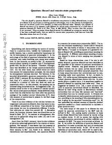
This quantity is zero if ρAB is classical-quantum, and positive otherwise. Can its value quantify the quantum correlations of ρAB ? Remarkably, in the limit of infinitely many ancillae, it has been proven in [20] that the quantity in Eq. (17) reproduces exactly the quantum discord given by Eq. (13) [see Figure 1(a)]: A

lim ∆(N) (ρAB ) = QIA (ρAB ) .

N→∞

(18)

This relation provides a striking operational understanding of quantum discord as the minimum average loss of correlations if one attempts to redistribute the correlations between A and B in the state ρAB to infinitely many ancillae on A’s side: paraphrasing the words of [21], “quantum correlations cannot be shared”. We note that additional operational interpretations for the quantum discord in quantum information theory and thermodynamics have been discovered, as reviewed in [3, 4, 5].

5 Alternative characterizations of quantum correlations So far we have focused on the characterization of classically correlated states and the quantification of quantum correlations in an entropic setting, using the quantum discord. One property that we have pointed out along the way is that the classically correlated states are insensitive to a local complete rank-one projective measurement, a hallmark feature of the classical world. It has also been shown that classically correlated states are the only ones that are locally broadcastable, another intuitive property arising from the inability to copy general quantum states. It turns out that there is a whole raft of equivalent defining properties for the classically correlated states, and that with each property comes another way to quantify the quantum correlations [5]. The quantum discord accounts for the loss of correlations due to local measurements, but it is just one of many ways to measure the quantum correlations of a state. We will outline two more key properties of classically correlated states in the following, along with the corresponding method of measuring quantum correlations.

5.1 Local coherence Recall that we define the incoherent states with respect to a reference basis {|ii}di=1 as P those diagonal in this basis, i.e., states that can be written as δ = di=1 pi |ii hi| for some probability distribution {pi }di=1 . Any state that is not diagonal in this basis is called coherent [24, 1]. Now let us consider a bipartite quantum system AB with local reference bases A B {|i A i}di=1 in A and {|j B i}dj=1 in B. States incoherent with respect to the product basis {|i A i ⊗ dA ,dB |j B i}i,j=1 can be written as

δAB ii

=

dA X dB X

pijAB |i A i hi A | ⊗ |j B i hj B |

(19)

i=1 j=1

for some joint probability distribution {pijAB }, while states incoherent in the local reference A basis {|i A i}di=1 are written as

δAB iq

=

dA X

piA |i A i hi A | ⊗ ρBi

(20)

i=1

for some probability distribution {piA } and with arbitrary states ρBi of subsystem B. We can say that these locally incoherent states are incoherent-incoherent and incoherentquantum, respectively. Take a look back at Eqs. (4) and (5) describing the classically 10

A

A1A2

AN …

ℰ A → A1 … AN B

(a) Local broadcasting

B

A

UA

A

classical correlations

ρ AB

|0 A’ ⟩

B

B

A’

A’

ρ෤ ABA’

(b) Entanglement activation

quantum correlations quantum entanglement

(c) Legend

Figure 1: Operational interpretations and quantification of quantum correlations. (a) Local broadcasting of correlations [Section 4]. Two quantum systems A and B are initially in an arbitrary bipartite state ρAB with generally classical and quantum correlations. If a local channel EA→A1 ...AN is applied to A which redistributes it into asymptotically many fragments A1 , ... , AN , then the only correlations remaining on average between each fragment Ai and subsystem B are classical ones, while quantum correlations, quantified by the quantum discord QIA (ρAB ), cannot be shared. This can be seen as a manifestation of quantum Darwinism [20]. (b) Scheme of a premeasurement interaction acting on subsystem A of a bipartite system AB, described as a local unitary U A on A, followed by a generalized control-NOT operation with an ancilla A0 (which plays 0 the role of a measurement apparatus). Provided A0 is initialized in a pure state |0A i, the output ABA0 0 pre-measurement state ρ˜ is always entangled along the AB : A split if and only if the initial state ρAB of the system is not classical-quantum, i.e., contains general quantum correlations from 0 0 the perspective of subsystem A [22, 23]. The minimum entanglement E AB:A (ρ˜ ABA ) between AB 0 and A in the pre-measurement state, where the minimization is over all the local bases on A specified by U A , quantifies the quantum correlations QEA (ρAB ) in the input bipartite state ρAB , according to the entanglement activation paradigm [Section 5.2]. (c) Graphical legend for the different types of correlations appearing in panels (a) and (b).

correlated states. You would be forgiven for thinking that they are identical to the equations given above! However, there is a subtlety here: the locally incoherent states are diagonal in a fixed local basis, while the classically correlated states are diagonal in some local basis. This analogy then provides us with another characterization of the classically correlated states, i.e. classical-classical states are incoherent-incoherent for some product basis on A and B, while classical-quantum states are incoherent-quantum for some local basis on A [5]. On the other hand, quantumly correlated states are coherent in every local basis. Can we then use measures of coherence to inform us on the amount of quantum corP relations? Consider the observable K = di=1 ki |ii hi| diagonal in a fixed reference basis {|ii}di=1 . One way to measure the coherence of a state ρ with respect to the reference basis, or more precisely its asymmetry with respect to translations generated by the observable K , is by means of the quantum Fisher information F (ρ, K ) [25, 26]. This quantity plays a fundamental role in quantum metrology [27] and indicates the ultimate precision achievable using a quantum probe state ρ to estimate a parameter encoded in a unitary evolution generated by the observable K . Let us now fix a family of local observables P A KΓA = di=1 kiA |i A i hi A | on subsystem A with fixed non-degenerate spectrum Γ = {kiA }di=1 . AB A B A Defining the minimum of F (ρ , KΓ ⊗ I ) over all local observables KΓ with spectrum Γ gives a measure of quantum correlations [28]: QFA (ρAB ) =

1 inf F (ρAB , KΓA ⊗ IB ). 4 KΓA

(21)

Such a measure embodies the worst-case scenario sensitivity of a bipartite state ρAB when a parameter is imprinted onto subsystem A by any of the observables KΓA : a process that is fundamentally linked to quantum interferometry and hence motivates the naming of QFA (ρAB ) as the interferometric power [28]. While there are many other good measures of quantum coherence [1], from which one can define corresponding mea11

sures of quantum correlations (by minimization over local reference bases) [5], the interferometric power is one of the most compelling as it brings together quantum coherence, quantum correlations, and metrology. Another advantage of this measure is that QFA (ρAB ) admits a computable formula for any state ρAB whenever A is a qubit [28], while no such analytical formula is presently available for the quantum discord QIA (ρAB ) of general twoqubit or qubit-qudit states.

5.2 Entanglement activation Let us now examine more closely the workings of a local projective measurement ΠA [ρAB ] = PdA A (Πi ⊗ IB )ρAB (ΠAi ⊗ IB ) with local projectors ΠAi = |i A i hi A | acting on subsystem A of a i=1 bipartite state ρAB . According to von Neumann’s model [29], this measurement can be realized in two steps. First, subsystem A is allowed to interact with an ancilla A0 , initial0 0 0 ized in a fiducial pure state |0A i h0A |, through a unitary U{|iAAA i} . The unitary acts in the following way 0 0 0 U{|iAAA i} |i A i ⊗ |0A i = |i A i ⊗ |i A i , (22) 0

0

0

and can be realized by the combination U{|iAAA i} = C AA (U{|iA A i} ⊗ IA ) of a local unitary U{|iA A i} which sets the basis of measurement, followed by a generalized controlled-NOT gate 0 0 0 0 C AA , whose action on the computational basis |i A i ⊗ |j A i of Cd ⊗ Cd is C AA |i A i ⊗ |j A i = A A0 |i i ⊗ |i ⊕ j i, with ⊕ denoting addition modulo d. The resultant state after applying the 0 unitary U{|iAAA i} to A, A0 and B is 0

0

0

0

0

ρ˜ ABA = (U{|iAAA i} ⊗ IB )(ρAB ⊗ |0A i h0A |)(U{|iAAA i} ⊗ IB )† , {|i A i}

(23)

which is known as the pre-measurement state. Next, the local projective measurement is completed by partial tracing over subsystem A0 , which is achieved by a readout of the 0 ancilla A0 in its eigenbasis, so that TrA0 ρ˜ ABA = ΠA [ρAB ]. {|i A i} 0 During this process the ancilla A can become entangled with A and B due to the 0 0 unitary U{|iAAA i} . which means that the pre-measurement state ρ˜ ABA may not be separable {|i A i} 0

along the bipartition AB : A0 . However, sometimes ρ˜ ABA remains separable along such {|i A i} cut. It turns out this is the case only when ρAB is initially incoherent-quantum, of the form in Eq. (20). It thus becomes clear that we can characterize the classical-quantum states of Eq. (5) as exactly all and only the states for which there exists a local basis {|i A i} such 0 that the pre-measurement state ρ˜ ABA is separable along the split AB : A0 [22]. {|i A i} Similarly, if we consider a local projective measurement (ΠA ⊗ ΠB )[ρAB ] on both A A B and B in the bases {|i A i}di=1 and {|j B i}dj=1 , we can also introduce an ancilla B 0 for B and 0 0 B a corresponding pre-measurement state ρ˜ ABA . A similar line of thought can then be {|i A i,|j B i} applied whereby we find that the classical-classical states of Eq. (4) are all and only the states for which the pre-measurement state is separable along the split AB : A0 B 0 for A B some local bases {|i A i}di=1 and {|j B i}dj=1 [23]. From this analysis, it can be said that the classical correlations are not always activated into entanglement during a pre-measurement, while the quantum correlations always are. Such a conversion of non-classical resources due to a pre-measurement interaction has been demonstrated experimentally in [30]. Naturally, one can then aim to quantify the quantum correlations of ρAB by measuring the entanglement of the corresponding pre-measurement state, via some chosen entanglement measure E, minimized over all local bases. For every suitable E, we can then define a corresponding (one-sided or two-sided)

12

measure of quantum correlations [22, 23] as follows [see Figure 1(b)] 0

0

), QEA (ρAB ) = inf E AB:A (ρ˜ ABA {|i A i} {|i A i}

QEAB (ρAB ) =

0

0

0

0

ABA B inf E AB:A B (ρ˜ {|i A i,|j B i} ).

(24)

{|i A i,|j B i}

One of the most remarkable features of this approach is that the measures so defined capture quantitatively the hierarchy of quantum correlations, as one has QEAB (ρAB ) ≥ QEA (ρAB ) ≥ E A:B (ρAB ) for any valid entanglement measure E and any bipartite state ρAB , with equalities on pure states ρAB = |ψAB i hψAB |. For instance, one may choose the relative entropy of entanglement [31] ERA:B (ρAB ) = inf S(ρAB ||σAB sep ),

(25)

σAB sep

as our entanglement measure, where S(ρ||σ) = Tr(ρ log ρ − ρ log σ) is the relative entropy and the minimization is over all separable states σAB sep of the form in Eq. (3). The corresponding measures of quantum correlations, obtained by specifying E as ER in Eqs. (24), are known respectively as relative entropy of discord (one-sided) and relative entropy of quantumness (two-sided). Interestingly, these measures have been proven equivalent to the following expressions [22, 23]: QEAR (ρAB ) = inf S(ρAB ||χAB cq ),

QEAB (ρAB ) = inf S(ρAB ||χAB cc ), R

χAB cq

χAB cc

(26)

with minimizations over the classical-quantum states of Eq. (5) and the classical-classical states of Eq. (4), respectively. This enriches the quantification of quantum correlations as potential resources for entanglement creation, with an additional geometric interpretation in terms of the distance3 from the set(s) of classically correlated states. In turn, such a geometric approach can be used a priori to quantify quantum correlations adopting different distance functionals, as reviewed in [32, 33, 5].

6 Desiderata for measures of quantum correlations We have identified several alternative yet equivalent characterizations of the classically correlated states, in particular providing links with other fundamental elements of quantum mechanics such as coherence [1] and entanglement [2]. With each characterization of the classically correlated states comes another way to measure quantum correlations. Given such a catalogue of measures [5], it is sensible to wonder what makes a good measure of quantum correlations? This question is typically answered by imposing a number of requirements that any such good measure should obey. Let us consider a one-sided measure Q A (ρAB ), defined by a real non-negative function acting on quantum states ρAB . One natural requirement is that • Q A (χAB cq ) = 0, i.e., that our measure is zero for classically correlated states. We should also expect that quantum correlations are not dependent upon the local bases of A and B, which manifests as invariance under local unitaries U A on A and U B on B, • Q A (ρAB ) = Q A ([U A ⊗ U B ]ρAB [U A ⊗ U B ]† ). As we have already pointed out, entanglement and quantum correlations become the same phenomenon for pure states |ψAB i, hence it is sensible to require that a measure of quantum correlations should reduce to a measure of entanglement for pure states, 3 Note

that the relative entropy is not strictly a distance because it is not symmetric in its arguments.

13

• Q A (|ψAB i) = E A:B (|ψAB i) for some entanglement measure E A:B (ρAB ). Similar desiderata can be imposed for two-sided measures of quantum correlations Q AB (ρAB ). However, so far we have not specified how our measure of quantum correlations should behave under dynamics of the system. In the case of entanglement, it is typically required that a measure should not increase under local operations and classical communication (LOCC) EAB , i.e., E A:B (EAB [ρAB ]) ≤ E A:B (ρAB ) [31, 2]. In other LOCC LOCC words, one should not be able to generate entanglement by LOCC, the archetypal operations that spatially separated laboratories are limited to. This requirement is typically called monotonicity, and finding a comparable one for quantum correlations is tricky. For one-sided measures, it can be required that any local operation on subsystem B should not be able to increase the quantum correlations from the perspective of subsystem A [22], that is, • Q A (IA ⊗ EB [ρAB ]) ≤ Q A (ρAB ) for any local operation EB on B. Unfortunately, this cannot be the only monotonicity requirement, since it only specifies the local operations on B. Identifying the most meaningful and complete set of operations under which a good measure of quantum correlations should be monotone is currently an open question. We point the reader to [5] for a deeper explanation.

7 Outlook We are going to be relying increasingly on the quantum world as technologies evolve during the 21st century, so it is certainly worthwhile to develop a good understanding of the quantum-classical boundary. In this manuscript we have focused on the most general type of quantum correlations between spatially separated parties. Whilst a promising topic, it is still very much in its infancy, with a plethora of interesting and open questions yet to be answered. From the theoretical side, perhaps the most pressing question is to identify a physically motivated set of “free operations” under which to impose monotonicity for measures of quantum correlations. This can be achieved by treating quantum correlations as a resource, within the framework of resource theories [34]. Experimentally, we have yet to witness compelling evidence for the practical role of quantum correlations beyond entanglement in relevant quantum technologies, even though proof-of-principle demonstrations, e.g. in the context of quantum metrology, are particularly promising [28]. In this respect, while the number of insightful operational interpretations for measures of quantum correlations has grown substantially in recent years [5, 35], killer applications are perhaps still waiting to be devised. It is hoped that by raising the awareness of these concepts within the wider quantum information community, we can begin to truly appreciate the foundational role and power of non-classical correlations beyond entanglement. There are still many topics within the study of quantum correlations that we have not had the opportunity to cover here. Foremost amongst which is the extensive research on their dynamics in open quantum systems, which shows that quantum correlations are generally more resilient than entanglement to the effects of typical sources of noise and decoherence [36, 37], a promising feature for any quantum technology. We have also neither discussed the role of quantum correlations in quantum computing [38, 39] and cryptography [40], nor the quantification of quantum correlations among more than two parties [41] or in continuous variable systems [42]. Nevertheless, there is a wealth of resources available to fill these gaps [3, 4, 5, 32, 33]. We hope to have passed on to the reader our enthusiasm for this young and blossoming field at the very core of quantum mechanics, and look forward to future progress.

14

References [1] A. Streltsov, G. Adesso, and M. B. Plenio, arXiv preprint arXiv:1609.02439 (2016). [2] R. Horodecki, P. Horodecki, M. Horodecki, and K. Horodecki, Rev. Mod. Phys. 81, 865 (2009). [3] K. Modi, A. Brodutch, H. Cable, T. Paterek, and V. Vedral, Rev. Mod. Phys. 84, 1655 (2012). [4] A. Streltsov, Quantum Correlations Beyond Entanglement and their Role in Quantum Information Theory (SpringerBriefs in Physics, 2015), arXiv:1411.3208v1. [5] G. Adesso, T. R. Bromley, and M. Cianciaruso, J. Phys. A: Math. Theor. 49, 473001 (2016). [6] H. Ollivier and W. H. Zurek, Phys. Rev. Lett. 88, 017901 (2001). [7] L. Henderson and V. Vedral, J. Phys. A: Math. Gen. 34, 6899 (2001). [8] M. Piani, P. Horodecki, and R. Horodecki, Phys. Rev. Lett. 100, 090502 (2008). [9] D. Cavalcanti and P. Skrzypczyk, arXiv preprint arXiv:1604.00501 to appear in Rep. Prog. Phys. (2016). [10] N. Brunner, D. Cavalcanti, S. Pironio, V. Scarani, and S. Wehner, Rev. Mod. Phys. 86, 419 (2014). [11] E. Schrödinger, in Mathematical Proceedings of the Cambridge Philosophical Society (Cambridge Univ Press, 1935), vol. 31, pp. 555–563. [12] A. Ferraro, L. Aolita, D. Cavalcanti, F. Cucchietti, and A. Acín, Phys. Rev. A 81, 052318 (2010). [13] S. Wu, U. V. Poulsen, K. Mølmer, et al., Phys. Rev. A 80, 032319 (2009). [14] D. P. DiVincenzo, M. Horodecki, D. W. Leung, J. A. Smolin, and B. M. Terhal, Phys. Rev. Lett. 92, 067902 (2004). [15] M. D. Lang, C. M. Caves, and A. Shaji, Int. J. Quant. Inf. 9, 1553 (2011). [16] S. Luo, Lett. Math. Phys. 92, 143 (2010). [17] H. Barnum, C. M. Caves, C. A. Fuchs, R. Jozsa, and B. Schumacher, Phys. Rev. Lett. 76, 2818 (1996). [18] W. K. Wootters and W. H. Zurek, Nature 299, 802 (1982). [19] D. Dieks, Phys. Lett. A 92, 271 (1982). [20] F. G. S. L. Brandão, M. Piani, and P. Horodecki, Nature Commun. 6, 7908 (2015). [21] A. Streltsov and W. H. Zurek, Phys. Rev. Lett. 111, 040401 (2013). [22] A. Streltsov, H. Kampermann, and D. Bruß, Phys. Rev. Lett. 106, 160401 (2011). [23] M. Piani, S. Gharibian, G. Adesso, J. Calsamiglia, P. Horodecki, and A. Winter, Phys. Rev. Lett. 106, 220403 (2011). [24] T. Baumgratz, M. Cramer, and M. B. Plenio, Phys. Rev. Lett. 113, 140401 (2014). [25] D. Girolami, Phys. Rev. Lett. 113, 170401 (2014). [26] I. Marvian and R. W. Spekkens, Nature Commun. 5, 3821 (2014). [27] S. L. Braunstein and C. M. Caves, Phys. Rev. Lett. 72, 3439 (1994). [28] D. Girolami, A. M. Souza, V. Giovannetti, T. Tufarelli, J. G. Filgueiras, R. S. Sarthour, D. O. Soares-Pinto, I. S. Oliveira, and G. Adesso, Phys. Rev. Lett. 112, 210401 (2014). [29] J. von Neumann, Mathematical Foundations of Quantum Mechanics (Springer-Verlag, Berlin, 1932).

15

[30] G. Adesso, V. D’Ambrosio, E. Nagali, M. Piani, and F. Sciarrino, Phys. Rev. Lett. 112, 140501 (2014). [31] V. Vedral, M. B. Plenio, M. A. Rippin, and P. L. Knight, Phys. Rev. Lett. 78, 2275 (1997). [32] D. Spehner, J. Math. Phys. 55, 075211 (2014). [33] W. Roga, D. Spehner, and F. Illuminati, J. Phys. A: Math. Theor. 49, 235301 (2016). [34] M. Horodecki and J. Oppenheim, Int. J. Mod. Phys. B 27, 1345019 (2013). [35] I. Georgescu, Nature Phys. 10, 474 (2014). [36] J. Maziero, L. C. Céleri, R. M. Serra, and V. Vedral, Phys. Rev. A 80, 044102 (2009). [37] L. Mazzola, J. Piilo, and S. Maniscalco, Phys. Rev. Lett. 104, 200401 (2010). [38] A. Datta, A. Shaji, and C. M. Caves, Phys. Rev. Lett. 100, 050502 (2008). [39] Z. Merali, Nature 474, 24 (2011). [40] S. Pirandola, Sci. Rep. 4, 6956 (2014). [41] C. C. Rulli and M. S. Sarandy, Phys. Rev. A 84, 042109 (2011). [42] G. Adesso and A. Datta, Phys. Rev. Lett. 105, 030501 (2010).

16