An Introduction to Statistics and Quantitative Methods

CHAPTER

1

AN INTRODUCTION TO STATISTICS AND QUANTITATIVE METHODS OUTLINE OF CHAPTER Variables and Probability Levels Introduction to Probability Hypotheses and Tests Generalization and Representativeness Correlation and Causation The Normal Distribution Summary Resource

1

2

PRACTICAL STATISTICS

B

efore we jump head-first into different statistical tests, we first must go over some important elementary topics so as to adequately introduce you to statistics. Without this knowledge, statistics may be used improperly: Wrong statistical tests may be selected for your data, which can lead to incorrect results, or other, similarly serious mistakes can be made. More simply, it is important to understand why statistics is important and how it is powerful before you start running statistical analyses.

VARIABLES AND PROBABILITY LEVELS First, you need to understand what statistics is used for. Statistics is used to provide evidence for (not prove) either a relationship or a lack of a relationship between two or more variables. A variable can consist of anything that can be measured. For example, a variable can be age, years of education, the number of times someone has seen a doctor in the past year, or measures of attitudes toward politics. As you can see, a variable can be directly measured (as in age or years of education) or can be a concept, which is only indirectly measured (such as people’s attitudes). The second point here is that with statistics, relationships can be suggested or shown, but not “proven.” With every statistical test, your results will include a probability level or p level. For example, say you are studying gender differences in income. You randomly select 400 people and ask their gender and income. Say the average income for males is about $23,000 and the average income for females is about $17,000. Despite this large difference in average income, we cannot definitively say, either with or without statistics, that men have higher incomes than women. This is because of the possibility of error. In this example, the men in our sample may just through chance have had higher than average incomes, and the females in our sample may have had lower than average incomes, again just through chance. In our results, the p level or probability level will tell us the probability that there is a true difference between groups as well as the probability that the differences that we see are simply due to this kind of error, or chance.

INTRODUCTION TO PROBABILITY In mathematics, the probability of something happening will always be between 0 and 1. The probability of an event occurring or not occurring

CHAPTER 1

AN INTRODUCTION TO STATISTICS AND QUANTITATIVE METHODS

will simply be its percentage divided by 100. Also, you’ll get rid of the percentage sign (%). For example: The chance of flipping a coin and getting heads = 50%. 50%/100 = .50 or 0.50 Here, the probability of flipping a coin and getting heads is .50. The chance of rolling a die and getting “6” = 16.67%. 16.67%/100 = .1667 or 1/6 Here, the probability of rolling a die and getting “6” is .1667 or 1/6. Shortly, I will present a small data set I constructed for this example, followed by the results of a statistical analysis (don’t get scared!) testing whether there is a gender difference in income. This data set consists of 10 males and 10 females, and as you can see from the data, I made it a point that males on average have higher incomes than females. Besides illustrating the concept of the probability level in statistics, this section will also give you an introduction to IBM® SPSS® Statistics and data sets. Just as a note, I will try throughout this book to have examples that use actual data. Also, I will as much as possible (beginning now) include actual screenshots and results from the software that you’ll be using when you do your statistical analyses. The software that is covered in this book includes IBM SPSS and Stata, which are two very popular general-purpose statistical analyses programs; HLM, which is a program that is used solely for hierarchical linear modeling, a specialized type of statistical test; and AMOS, which is used for structural equation modeling, an advanced statistical model. So here is our data set. This screenshot comes from IBM SPSS. While we will cover these different statistical software packages more later on, I will include some basic notes here as we go along. You may find that IBM SPSS is more convenient than Stata for entering data (e.g., if you gave a survey, we would first have to enter the data into a software program before you can do an analysis). So let’s take a look at this. You can see that on top there are two variables, “sex” and “yincome.” In your data sets, as in this one, each variable will have its own column. On the left, we see a column of numbers, with the numbers 1 through 20. The 20 numbers (called “case numbers” when discussing data sets) correspond to the 20 individuals whose data we have.

3

4


The first variable, “sex,” measures the person’s sex (in statistics, we call the individuals who make up a data set “respondents” or “participants”). In data sets, to run an analysis, everything needs a numerical or number code, even things such as sex, the region of the country you live in, or the highest degree you have. In this case, we chose “0” to stand for females and “1” to stand for males. In the case of “yincome,” the number represents the respondent’s yearly income in dollars. You may find it more convenient to give variables short (eight characters or less) but descriptive names, as older versions of Stata only support variables with eight characters or less in their name. If you were to import a file from IBM SPSS into an older version of Stata that contains variables with more than eight characters in their names, everything will work, but the names of the variables will be truncated to eight characters, which might make things confusing. AMOS and older versions of IBM SPSS have this same limitation. In general, it is a good rule to always limit variable names to eight characters or less. OK, now for the analysis. For now I’ll skip over how to do the analysis, as I will cover this in much detail in a later chapter. However, I will include a

CHAPTER 1


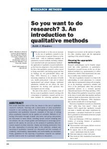
screenshot of results to illustrate the concept of the probability level. Just as a note, to analyze this data, we will conduct what is called a t-test (Figure 1.1). Don’t let this scare you: By the time you have finished reading this book, you will easily understand the meaning of this output. In this example, we find that the probability level under the fifth column of numbers, labeled “Sig. (2-tailed).” Here, it is “.000.” However, in statistics, the probability level can never be 0, because there is always some chance that our findings are due to error. What IBM SPSS means is our probability level is very very low, below .001. When IBM SPSS finds the probability to be below .001, it gives “.000” as your result. Keep in mind that this is just a minor “bug” in IBM SPSS; in reality, your probability level can be extremely small, but it can never be 0. So we know that our probability level is less than .001. But that mean? It means that the probability that the differences in income that we saw based on gender are due to chance, or random variation, is less than .001. Conversely, there is a greater than .999 probability that the differences we saw based on gender in income are due to a real, genuine difference (due to, say, differences in level of education, discrimination, etc.). Basically, there’s a greater than .999 probability that this difference is not due to our having happened to have picked males who had very high incomes and/or females who had very low incomes. In social science, you will see these three standards for the probability level: .05, .01, and .001. A probability level of .05 means that there is a 95% chance that there is a real relationship between the variables and a 5% probability that the difference is due to error or chance. The .05 standard is the one most commonly used in the social sciences;

Figure 1.1

Probability Levels: Example of a t-test in SPSS

5

6

PRACTICAL STATISTICS however, if your probability level is lower than one of the stricter standards (.01 or .001), then that is what would be noted in a research paper or study. To illustrate, in the example above, we had a probability level of less than .001. If we were writing these results in a research paper, we could say something such as the following: The relationship between gender and income was statistically significant, with males tending to have higher incomes than females ( p < .001). The term statistically significant simply refers to the fact that our probability level was less than .05, the standard. We have also noted that our calculated probability level, represented as p, was less than .001. We note that the probability level is less than .001 instead of using the .05 or .01 standards as it is customary to include only the strictest standard that is met. In statistics, the probability level will always refer to the probability that the difference or relationship that you see is due to chance. To come up with the probability that the difference or relationship is not due to error or chance, you just need to subtract the probability level from 1. For example: If our probability level (the probability it was due to chance) = .07 (or 7%). The probability that the difference is a real effect = 1 − .07 = .93 (or 93%).

HYPOTHESES AND TESTS In the example above, where we tested gender differences in income based on a hypothetical data set, we also tested a hypothesis. When you run a statistical analysis, you’ll typically be testing one or more hypotheses. A hypothesis is a prediction about the relationship between two or more variables. For example, when we tested the relationship between gender and income, our hypothesis may have been: Males are more likely to have higher incomes than females. Here are some more examples of hypotheses: It is predicted that males are more likely to vote Republican than females. It is predicted that high levels of frustration lead to heavy alcohol use, which in turn leads to unprotected sex. We can use statistical tests to test these and all sorts of other hypotheses. A very important point here is that a particular type of statistical test will be most appropriate depending on your hypothesis and the nature of your data.

CHAPTER 1


While several different types of statistical tests may be appropriate, there will be some that will be very inappropriate. It is important to consider your hypotheses and data and come to a correct decision based on your hypothesis and the nature of your data. While I’m simply noting this now as part of the introduction, a guide to determining which test to use on the basis of the nature of your hypothesis and data is included in Appendix A. This is a crucial issue and one which can lead to serious errors if not considered appropriately. As a quick example, in the analysis above, I chose to do a t-test; more specifically, an independent samples t-test. This type of test happens to be appropriate because we’re looking at the difference between two groups, males and females (if you’re looking at the difference between three or more groups, you would do an ANOVA), and because the dependent variable, the variable we’re trying to predict (income), is continuous (not a number of categories). Variables that we use to predict our dependent variable are called independent variables. In this case, our independent variable is sex or gender. If our data were different, or our hypothesis (what we were trying to test) was different, we would probably use a different statistical test. This issue will be covered throughout the text.

GENERALIZATION AND REPRESENTATIVENESS The concepts of generalizability and randomness are the most important, yet some of the most neglected, in the field of statistics. First, we will cover the concept of a random sample. A random sample does not mean you got a group of “random people” that you gave a survey to on the street or in a mall. In statistics, a random sample means a very specific and particular thing. A random sample means that every person in your population has an equal chance of being selected for participation in your study. When conducting research, a sample refers to the group of people you select for study, while a population refers to a larger body of individuals from whom you selected your sample and who you wish to be able to describe using the results of your study. For example, say that your population is adults living in the United States. In doing your study, you wish the results of your study to be generalizable to this population. If your study was to be generalizable to all adults living in the United States, it would mean that you can apply the results of your study to all adults living in the United States. This is one of the most powerful elements of statistics. Your study may only consist of 50 or 100 individuals; however, if it is a random sample, you can apply your results to the entire population (in this example, all the adults living in the United States). In this way, our sample is representative of our population.

7

8

PRACTICAL STATISTICS Take as an example, the analysis between gender and income that was presented earlier in this chapter. If this sample of nearly 20 individuals was a random sample of adults in the United States (i.e., if every adult living in United States had an equal chance of being selected for the survey), we could say that not only do these 10 males have a significantly higher income than the 10 females we selected in our survey, but that on average, adult males in the United States have higher incomes than adult females. By using this method of sampling combined with statistical tests, we are able to extend our results based on 20 individuals to millions of individuals. Keep in mind that representativeness and generalizability work both ways. If you do not have a random sample (if it is not true that every member of the population has an equal chance of being selected for your study), then your sample is not representative of the population and you cannot generalize your results to the population at hand. So if you stand on a busy sidewalk and recruit 40 people to fill out a survey, when you discuss your results, you can only talk about those 40 people, because you did not have a random sample. You cannot generalize the results to people in general, Americans in general, adults in general, the population of that town, and so on. This is a crucial point that even some famous researchers do not take into account, and it is a grievous error.

CORRELATION AND CAUSATION A very important concept in quantitative methods is the distinction between correlation and causation. The term correlation refers to the relationship between two variables (i.e., how related they are). A distinct concept is that of causation, which signifies that one variable causes another one to change. Just because two variables are correlated (i.e., related) does not necessarily mean that they are related causally (i.e., that one causes the other). This is an extremely important concept in quantitative methods. Take the example of the relationship between watching violent television and being violent among youth. Say you found that there was a relationship between watching violent television and expressing violent behavior such that children who spend more time watching violent television also express more violent behavior. Here, we know that these two factors are correlated: that there is a relationship between the two variables of time spent watching violent television and violent behavior. However, we know nothing about whether watching violent television in fact causes violent behavior. Therefore, we cannot say whether these two factors are causally related. Providing evidence for a correlation or relationship between two variables is very easy, but

CHAPTER 1


providing evidence that two variables are causally related (that one in fact causes the other) is significantly more difficult. The key concept to remember here is a phrase that you might hear in your first statistics course: “Correlation does not imply causation.” This phrase simply means that having a relationship or correlation between two variables says nothing about whether one in fact causes the other.

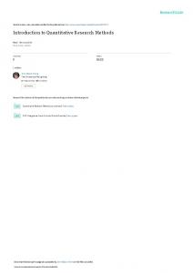
THE NORMAL DISTRIBUTION A normal distribution describes data that are distributed in a certain type of way. In essence, in data that are normally distributed, the majority of cases (e.g., of years of education, attitude measurements, etc.) will be close to the average value, and the further away you get from the average value, the fewer cases you will see. An example of something that is normally distributed is height. The height of most people is around the average, which is approximately 5 feet 7 inches when including both males and females. While the majority of individuals have a height close to this value, there are still a fair degree of individuals who are substantially taller or shorter than this average, say around 6 feet 6 inches or 4 feet 8 inches. As you continue traveling further from this average, you see fewer and fewer individuals. There are some individuals who are 7 feet tall or 4 feet tall, but they are very rare. Likewise, there are even some individuals who are 8 feet tall or 3 feet tall, but they are even more rare. Pictorially, a graph of human height versus the number of individuals with that height would look like Figure 1.2. The shape of this graph is called a “bell curve” and resembles what any normally distributed variable would look like. As the graph illustrates, the majority of people are around the average height of 160 cm. As you get further and further away from this average, we see fewer and fewer people. IQ (intelligent quotient), which is also a normally distributed variable, would look like Figure 1.3. Here, we see that the average is 100, and the further we get away from this average, the fewer people there are. A number of the statistical tests that are discussed in this book make the assumption that the dependent variable, the variable that you are trying to predict, is normally distributed. If you use one of these tests with data that are not normally distributed, it may or may not be an issue. The area of assumptions, testing assumptions, and what to do when an assumption has been violated is a very complex and nuanced area and is not the focus of this book. In statistics classes that you take, you may be given the simple instruction of performing an alternative test when an assumption has been violated. This is

9


prob. per unit height (cm−1)

0.03

0.02

0.01

0.00 120

140

160

180

200

height (cm)

Figure 1.2

The Normal Distribution: Height

IQ Score Distribution 34% Percentage of Population

10

34%

68% 14%

14%

95%

2%

0.1% 55

70

85

100

2% 115

130

0.1% 145

IQ Score

Figure 1.3

The Normal Distribution: IQ Scores

an overly simplistic view of the issue of assumptions and assumption violation and really does more harm than good. In regard to certain assumptions of certain tests, violation may not really be an issue at all. In other cases, it may be. Whether it is or not depends on the particular assumption and the particular test and how badly the assumption has been violated.

CHAPTER 1


11

If you are more interested in the subject of testing variables for normality (whether they are normally distributed or not), please see Section 3 of Appendix C.

SUMMARY This chapter provided a brief but important introduction to statistics and quantitative methods. First, the purpose of statistical tests was discussed. Statistical tests are used to provide evidence for or against a relationship between two or more variables. Variables can consist of anything that can be measured. Most analyses consist of a single dependent variable and multiple independent variables. Your dependent variable is the variable which you are trying to predict or explain, while your independent variables are the variables that you use to predict your dependent variable. Next, the concept of the probability level was introduced. The probability level is an indicator that measures the level of certainty that a finding was in fact due to a real relationship between variables versus the probability that it is simply due to error or chance. Next, the concept of the hypothesis was introduced, which is a prediction about the relationship between two or more variables. Based on your hypothesis and the nature of your data, you will select the appropriate statistical test to perform in order to test your hypothesis. Selecting the appropriate statistical test is vital to avoid errors, and while this process is simple even with a basic knowledge of statistics, it is commonly incorrectly done. The next section of this chapter introduced the concept of generalizability. To be able to generalize your findings to the larger population, you must use a random sample that is representative of the larger population. Finally, many variables in the social sciences are normally distributed, in which most cases are close to the average score, and the further you get from the average the fewer cases you see (the “bell curve”). The next chapter will introduce the reader to two very popular, generalpurpose statistical software packages, IBM SPSS and Stata. Chapter 2 will also present directions on how to enter data into both of these programs, which would be the first step of your data analysis if you were not using a preexisting data set.

RESOURCE This book’s Web site can be found at the following location: www.sagepub .com/kremelstudy