An Investigation into a Neural Network's performance ...

AIAA 2006-3330

24th Applied Aerodynamics Conference 5 - 8 June 2006, San Francisco, California

An Investigation into a Neural Network’s performance based on the Number of Neurons in the Hidden Layer Timothy Scully$, Kelly Cohen*

Downloaded by UNIVERSITY OF CINCINNATI on December 2, 2014 | http://arc.aiaa.org | DOI: 10.2514/6.2006-3330

Department of Aeronautics US Air Force Academy US Air Force Academy, CO 80840

An important benchmark for closed-loop flow control is the suppression of the von Kármán vortex street in the wake of a circular cylinder at a Reynolds number of 100. A low-dimensional Proper Orthogonal Decomposition (POD) is applied to the flow field and a four sensor configuration is placed based on the intensity of the resulting spatial Eigenfunctions. This effort focuses on the performance of a non-linear Artificial Neural Network Estimator (ANNE) used for real-time mapping of flow field sensors to POD states. This investigation examines the sensitivity of ANNE by varying the number of neurons in the hidden layer. The aim is to determine if there is an optimum number of neurons in the hidden layer. Three input data sets were studied, the first had no noise on the training and testing data, the second had 10% noise applied to the training and testing data, and the third had 25% noise applied to the training and testing data sets. In all cases 50 randomly selected training data sets were applied to the back-propagating network. A separate data set was used for testing the feed-forward network. During the validation process, network outputs were compared to desired outputs and the Root Mean Squared (RMS) error was calculated for each of the four output nodes. Results show that in general, the more nodes in the hidden layer the better the performance of the network. However, there appeared to be a consistently reduced error when eight (8) nodes were used in the hidden layer. Results from ANNE when compared to the state-of-the-art Linear Stochastic Estimator (LSE) shows significant benefits.

I. Introduction One of the main purposes of flow control is the improvement of aerodynamic characteristics of air vehicles and munitions enabling augmented mission performance. An important area of flow control research involves the phenomenon of vortex shedding behind bluff bodies. These bodies often serve some vital operational function. Their purpose is not to augment aerodynamic efficiency and often aerodynamic performance is sacrificed for functionality. Flow separates from large section of the bluff body’s surface. The resulting wake behind the bluff body, known as a vortex street, exhibits vortex shedding, which then leads to a sharp rise in drag, noise and fluid-induced vibration (Gillies, 1998)1. The ability to control the wake of a bluff body could be used to reduce drag, increase mixing and heat transfer, and enhance combustion. Shedding of counter-rotating vortices is observed in the wake of a two-dimensional circular cylinder bluff body above a critical Reynolds number (Re ~ 47, nondimensionalized with respect to freestream speed and cylinder diameter). This phenomenon is often referred to as the von Kármán vortex street (von Kármán, 1954)2. Drag, noise and vibration reduction are possible by controlling the wake of a bluff body. In the past decade or so, active closed-loop flow control has been found to be an effective means for suppression of self-excited flow oscillations without geometry modification (Park et al, 1993)3.

$ Assistant Professor, Department of Aeronautics, US Air Force Academy, Member, AIAA * Contracted Research Engineer, Department of Aeronautics, US Air Force Academy, Senior Member, AIAA

1 American Institute of Aeronautics and Astronautics This material is declared a work of the U.S. Government and is not subject to copyright protection in the United States.

Downloaded by UNIVERSITY OF CINCINNATI on December 2, 2014 | http://arc.aiaa.org | DOI: 10.2514/6.2006-3330

Low-dimensional modeling is a vital building block when it comes to realizing a structured model-based closed-loop strategy for flow control. For control purposes, a practical procedure is needed to break down the velocity field, governed by Navier Stokes partial differential equations, by separating space and time. A common method used to substantially reduce the order of the model is proper orthogonal decomposition (POD) (Cohen et al, 2006)10. This method is an optimal approach in that it will capture a larger amount of the flow energy in the fewest modes of any decomposition of the flow. A major challenge in implementing POD modeling is real-time estimation of the POD states. The state-of-the art technique is based on Linear Stochastic Estimation (LSE) first introduced by Adrian (1977)4. Sensor measurements may take the form of wake velocity measurements, as in this effort, or for an application based on surfacemounted pressure measurements and/or shear stress sensors. This process leads to the state and measurement equations, required for design of the control system. In this effort we introduce a non-linear Artificial Neural Network Estimator (ANNE) used for real-time mapping of flow field sensors to POD states. In developing an effective neural network, the hidden architecture is often arrived at based on experience and judgment. Few rules concerning the number of hidden layers and number of neurons in those layers exist. However, the performance of a neural network is definitely affected by these two parameters (number of hidden layers and number of neurons in each hidden layer). Some indication of the relationship of hidden units to network performance is given in Mourrain et al, (2004)8, which indicates that the performance of the network is influenced by the number of hidden nodes. However, this paper does not provide any quantifiable relationship between network performance and number of hidden layers or number of nodes in those layers. Mourrain et al, (2004)8 indicated that performance can be adversely impacted by not enough hidden nodes but does not speak to the impact of an excessive number of hidden nodes. Generally, the fewer the number of hidden nodes, the better a network is able to generalize. The reverse is, the more hidden nodes a network has, the higher the probability the network will learn individual input patterns and generate an output based on a specific input. This represents the opposite of generalization and is not considered a desirable trait of an artificial neural network. The number of hidden nodes is sometimes related to the number of training data sets. For example, if few data sets are available for training, only a few neurons would be used in the hidden layer to improve the networks ability to generalize. Up to this point, words like “few”, “more”, and “generalize” have been used to effort to quantify the number of hidden neurons in an artificial neural network. What follows is an attempt to define a specific number of hidden nodes that provides exceptional performance for a back-prop network in a specific application.

II. Research Objective In the application of Neural Networks often the number of nodes in the hidden layer is chosen to be something greater than the number of input nodes but without regard to the “cost” (reduced error verses implementation complexity) of the network. Although this approach is simple and easy to implement, it is important to consider various cost factors when selecting the number of hidden neurons. The main objective of this research effort is to determine for a specific application, if there is a exact number of hidden neurons that yields exceptional performance and to then develop a systematic approach for determining that optimum number of nodes in the hidden layer of an Artificial Neural Network Estimator (ANNE). Results using ANNE will be compared to the baseline LSE approach. Finally, a cost model based on output error and number of hidden nodes will be proposed.

2 American Institute of Aeronautics and Astronautics

Downloaded by UNIVERSITY OF CINCINNATI on December 2, 2014 | http://arc.aiaa.org | DOI: 10.2514/6.2006-3330

III. Application - High Resolution Computational Model If a specific number of hidden nodes can be found to provide superior performance in a neural network, that configuration may be application specific. A description of the application used for this trial follows (Cohen et al, 2006)5: A simple model of the flow-field was sought to design sensor configurations for feedback control algorithms. The model primarily needs to accurately capture the dynamic behavior of the flow field and this need to be verified with experimental data presented in the literature. Numerical simulations were conducted on Cobalt Solutions COBALT solver V.2.02. In this effort, the above solver was used for direct numerical solution of the Navier Stokes equations with second order accuracy in time and space. An unstructured two-dimensional grid with 63700 nodes and 31752 elements was used. The grid extended from –16.9 cylinder diameters to 21.1 cylinder diameters in the x (streamwise) direction, and ±19.4 cylinder diameters in y (flow normal) direction. Additional simulation parameters are as follows: • Two-dimensional cylinder, diameter = 1m • Reynolds Number (Re) = 100 (ideal gas) • Laminar Navier-Stokes equations • Vortex shedding frequency – 5.55Hz. • Mean flow, U= 34 m/s • Damping Coefficients: Advection = 0.01; Diffusion = 0.00 • 32 Iterations for matrix solution scheme • 3 Newtonian sub-iterations • Pressure = 4.337 Pascal • Density = 0.0000525 Kg/m3 • Non-dimensional time step, Δt*=Δt.U/D= 0.05 • Time step, Δt = 0.00147 s. The simulation was triggered by skewing the incoming mean flow by α = 0.5 degrees to introduce an initial perturbation. For validation of the unforced cylinder wake CFD model at Re = 100, the resulting value of the mean drag coefficient, Cd, will be compared to experimental and computational investigations reported in the literature. The CFD model, used in this effort results in a Cd =1.35 at Re = 100, which compares well with the reported literature. Another important benchmark parameter concerns the value of the non-dimensional Strouhal number (St) for the unforced cylinder wake. Experimental results at Re = 100, point to St values of 0.167- 0.168. The CFD model, used in this effort, has a St = 0.163 at Re = 100 which also compares well with the reported literature.

IV. Sensor Configuration and Linear Stochastic Estimation For each sensor configuration, 138 velocity measurements were used equally spaced at 0.00735 seconds apart. All the measurements were taken after ensuring that the cylinder wake reached steady state. Of the 138 snapshots, the first 70 were used for training of LSE/ANNE, whereas, the final 68 snapshots were used for validation purposes. Only data concerning velocity components in the direction of the flow were used for the sensor placement and number studies reported in this effort. The effectiveness of a linear mapping between for velocity measurements and POD states has been experimentally validated by Cohen et al. (2006)5 For a given sensor configuration, the effectiveness of the linear stochastic estimation process for the estimation of the first four temporal mode amplitudes is calculated. The extracted mode amplitudes are obtained by introducing the spatial Eigenfunctions into the snapshot data of the velocity field using the least squares method. For sake of convenience, this RMS error is normalized with the RMS of the desired extracted mode amplitudes, presented as a percentage. The resulting error percentage and the number of sensors may be integrated together into a cost function and the purpose of the design process would then be to select the configuration that minimizes this cost. The issue of sensor placement and number has been dealt with in detail by Cohen et al (2006)5 for the same data as used in this study and therefore in this effort the sensor configurations developed there are utilized.

3 American Institute of Aeronautics and Astronautics

V. Artificial Neural Network Estimator (ANNE)

Downloaded by UNIVERSITY OF CINCINNATI on December 2, 2014 | http://arc.aiaa.org | DOI: 10.2514/6.2006-3330

The neural network for this investigation was a fully connected back-propagating, single hidden layer artificial neural network with 4 input nodes and 4 output nodes as provided by MatLab based on Nørgaard et al’s(2000)7 toolbox. The Mat Lab provided a supervised learning scheme was used without modification with the back propagation based on the Levenberg-Marquardt algorithm. The activation function was chosen to be hyperbolic tangent (tanh).

Figure 1. Schematic of fully connected ANNE

Each input node represented the velocity output of an actual sensor in the flow field (Fig 1). A snapshot of all sensor outputs was applied to the input of the neural network representing one data (training or testing) set. A single hidden layer was selected for all scenarios for this investigation. The number of hidden neurons varied from four to 30. The number of hidden neurons was increased from four to 16 by a single neuron for each trial then a trial was accomplished with 30 hidden neurons. There were four output nodes. The output of each node represented the POD state based on the input.

4 American Institute of Aeronautics and Astronautics

To summarize, the network was designed to predict the POD state behind a circular cylinder given observations taken from the downstream wake.

Extracted Mode Amplitudes Projected on the ANNE Estimates 30

U Velocity Mode Amplitudes

Downloaded by UNIVERSITY OF CINCINNATI on December 2, 2014 | http://arc.aiaa.org | DOI: 10.2514/6.2006-3330

20

10

0

-10

Ext. Mode 1 Ext. Mode 2 Ext. Mode 3 Ext. Mode 4 ANNE Mode 1 ANNE Mode 2 ANNE Mode 3 ANNE Mode 4

-20

-30 2.55

2.6

2.65

2.7

2.75

2.8 Time [s]

2.85

2.9

2.95

3

3.05

Figure 2 Extracted Mode amplitudes projected using ANNE based on a four sensor configuration

Training the network was accomplished by applying a time slice of observational data to the network and then adjusting the network’s output to be in line with the desired output. Training occurred by taking random input data sets from a pool of 70 sets available. Training was limited to 100 trials for each configuration of the network. Once training was complete, test data was randomly applied to the network with the actual network output being compared to the desired output. A network performance figure of merit was arrived at – the Root Mean Squared (RMS) of the difference between all the actual outputs and all of the desired outputs. This process was repeated for three categories of input data –0%, 10%, and 25% “noise” attached to it. The addition of noise was accomplished by independently adding random noise (on an interval of -0.5 to 0.5) with amplitude of a percentage (RN Factor) of the freestream velocity to each of the sensor readings. The noise was generated randomly using MATLAB and separately for each individual sensor to prevent cancellation of the noise due to being in phase with noise at other sensor locations. Two levels of noise were studied, RN Factor 10% and RN Factor 20%. The estimated verses desired mode amplitude plot for the above sensor configuration is presented in Figure 2.

5 American Institute of Aeronautics and Astronautics

Testing the network was accomplished using 68 sets of input data (not used for training). The normalized RMS error in [%], for the 4 mode for each case was then calculated.

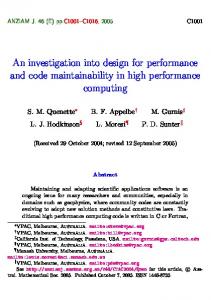
ANNE Performance 70

0.4

10% Noise No Noise

0.25 40 0.2 30 0.15 20

0.1

10

0.05

0

0 0

5

10

15

20

25

30

35

# Hidden neurons

Figure 3: RMS (%) of Estimation Errors vs. Number of Hidden Neurons in ANNE

Figure 3 shows the performance of the network with various number of hidden nodes. This figure shows that at 8 neurons in the hidden layer good performance is reached.

6 American Institute of Aeronautics and Astronautics

% RMS error (no noise)

0.3

50

% RMS error %(noise) RMS error

Downloaded by UNIVERSITY OF CINCINNATI on December 2, 2014 | http://arc.aiaa.org | DOI: 10.2514/6.2006-3330

0.35

25% Noise

60

Downloaded by UNIVERSITY OF CINCINNATI on December 2, 2014 | http://arc.aiaa.org | DOI: 10.2514/6.2006-3330

Table 1. RMS Error for Different Number of Nodes in the Hidden Layer.

Number of Hidden Nodes

RN Factor 0%

RN Factor 10%

RN Factor 25%

4 5 6 7 8 9 10 11 12 13 14 15 16 30

0.36 0.32 0.24 0.33 0.21 0.26 0.26 0.25 0.24 0.24 0.23 0.25 0.24 0.20

18.18 24.53 29.85 13.41 9.66 12.09 10.71 14.46 7.85 17.70 15.16 12.55 12.63 19.13

58.72 28.44 52.38 60.13 27.04 36.81 32.26 25.15 51.19 34.92 26.33 31.05 40.66 30.24

VI. Conclusions and Recommendations The results of this study can not be summarized by saying more hidden nodes provide better neural network performance. Nor can it be said that fewer is better. In the no noise case, 8 hidden nodes was the top performer of those configurations tested up to 16 hidden nodes. The case of 30 hidden nodes actually performed slightly better than 8 hidden nodes however the difference between the two is to small to be statically significant. All configurations (no noise, 10% noise, and 25% noise) showed some oscillation in performance at the lower number of hidden nodes. Based on a previous experimentally validated sensor placement Cohen et.al (2003)9, the sensitivity of the architecture of a neural network estimator (ANNE) was examined to minimize RMS estimation errors. The development of the procedure was based on CFD simulations of a cylinder at a Reynolds number of 100.The hidden architecture of an ANNE used in the application described above can be adjusted to affect performance of the ANNE. When noise was added, a preferable number of hidden neurons was still apparent however the number went up when compared to the number in the no-noise case. Further research will aim at examining the robustness of the proposed number of hidden neurons for the given application in the presence of sensor failure. Will there still be a specific number of hidden neurons that offers exceptional performance in the face of input sensor failure? If there is a particular hidden neuron configuration that works best? Is it the same number of neurons as in the “all inputs working” case? Furthermore, we would like to examine the sensitivity of ANN architecture to performance as a function of computational cost. While it appears premature to claim a heuristic for determination the optimum number of hidden nodes in a neural network, the investigation does point to a relatively small number of hidden nodes providing improved performance. With a manufacturing cost function in mind that values the number of connections in an integrated circuit, this result is obviously desirable.

7 American Institute of Aeronautics and Astronautics

References

Downloaded by UNIVERSITY OF CINCINNATI on December 2, 2014 | http://arc.aiaa.org | DOI: 10.2514/6.2006-3330

1

Gillies, E. A.., “Low-dimensional Control of the Circular Cylinder Wake”, Journal of Fluid Mechanics, Vol. 371, 1998, pp.157, 178. 2 von Kármán, T., Aerodynamics: Selected Topics in Light of their Historic Development, Cornell University Press, Ithaca, New York, 1954. 3 Park, D.S., Ladd, D.M., and Hendricks, E.W., “Feedback Control of a Global Mode in Spatially Developing Flows”, Physics Letters A, Vol. 182, 1993, pp. 244, 248. 4 Adrian, R.J., “On the Role of Conditional Averages in Turbulence Theory”, In Proceedings of the Fourth Biennial Symposium on Turbulence in Liquids, J. Zakin and G. Patterson (Eds.), Science Press, Princeton, 1977. 5 Cohen, K., Siegel, S., and McLaughlin, T.,"A Heuristic Approach to Effective Sensor Placement for Modeling of a Cylinder Wake”, Computers & Fluids, Vol. 35, Issue 1 , January 2006, pp. 103, 120. 6 Nelles, O., Nonlinear System Identification, Springer-Verlag, Berlin, Germany, 2001, Chap. 11. 7 Nørgaard, M., Ravn., O., Poulsen, N.K., and Hansen, L.K., Neural Networks for Modeling and Control of Dynamic Systems, 3rd printing, Springer-Verlag, London, U.K., 2003, Chap. 2. 8 Bernard Mourrain, Nicos G. Pavlidis, Dimitris K. Tasoulis, and Michael N. Vrahatis “Computing the Number of Real Roots of Polynomials through Neural Networks”, ICNAAM-2004 Extended Abstracts 3 . 5 9 Cohen, K., Siegel S., and McLaughlin T., "Sensor Placement Based on Proper Orthogonal Decomposition Modeling of a Cylinder Wake", 33rd AIAA Fluid Dynamics Conference and Exhibit, Orlando, Florida, AIAA Paper 20034259, June 23-26 2003 10 K. Cohen, S. Siegel, J. Seidel, and T. McLaughlin, 'Neural Network Estimator for Low- Dimensional Modeling of a Cylinder Wake', 3rd AIAA Flow Control Conference San Francisco, 5-8th June 2006, AIAA-2006-3491, 2006

8 American Institute of Aeronautics and Astronautics