An Investigation of Spectral Restoration Algorithms for Deep Neural Networks based Noise Robust Speech Recognition Bo Li1 , Yu Tsao2 , Khe Chai Sim1 1
2
School of Computing, Computing 1, National University of Singapore, Singapore Research Center for Information Technology Innovation (CITI), Academia Sinica, Taipei, Taiwan
[email protected],
[email protected],
[email protected]
Abstract Deep Neural Networks (DNNs) are becoming widely accepted in automatic speech recognition (ASR) systems. The deep structured nonlinear processing greatly improves the model’s generalization capability, but the performance under adverse environments is still unsatisfactory. In the literature, there have been many techniques successfully developed to improve Gaussian mixture models’ robustness. Investigating the effectiveness of these techniques for the DNN is an important step to thoroughly understand its superiority, pinpoint its limitations and most importantly to further improve it towards the ultimate human-level robustness. In this paper, we investigate the effectiveness of speech enhancement using spectral restoration algorithms for DNNs. Four approaches are evaluated, namely minimum mean-square error spectral estimator (MMSE), maximum likelihood spectral amplitude estimator (MLSA), maximum a posteriori spectral amplitude estimator (MAPA), and generalized maximum a posteriori spectral amplitude algorithm (GMAPA). The preliminary experimental results on the Aurora 2 speech database show that with multi-condition training data the DNN itself is capable of learning robust representations. However, if only clean data is available, the MLSA algorithm is the best spectral restoration training method for DNNs. Index Terms: speech enhancement, spectral restoration, deep neural networks.
1. Introduction Developing systems that would be much more robust against variability and shifts in acoustic environments, reverberations, external noise sources, communication channels, speaker and language characteristics has always been the goal of speech recognition researchers. In recent years, Deep Neural Networks (DNNs) have been successfully applied to various speech tasks, such as context-independent phoneme recognition [1, 2] and context-dependent large vocabulary speech recognition [3]. The DNN system has been shown to be capable of reducing the word error rate (WER) by up to one third on a challenging conversational speech transcription task compared to the discriminatively trained Gaussian mixture model (GMM) systems in [4]. This further intrigues the interest of adopting DNNs for the noise robust speech recognition. In [5], the Recurrent Neural Network (RNN) and the DNN have been shown to generalize much better than GMMs and MLPs on the Aurora 2 task [6]. In [7], a deep recurrent denoising autoencoder (DRADE) is trained on the stereo data to reconstruct the clean utterances from the noisy input features. It has been shown to outperform the SPLICE denoising algorithm [8] and the hand-engineered ETSI2 advanced front end (AFE) denoising system [9]. More-
over, DNNs trained from noisy data, i.e. the multi-condition trained DNNs, yield even better results and outperform GMM systems with various compensation techniques [10, 11]. However, both the DRADE and the multi-condition trained DNN are more dependent upon the training data to provide a reasonable sample of noise environments that could be possibly encountered at test time. This may limit the DNN performance due to the lack of heterogeneous data. Speech enhancement techniques that aim to reduce background noise from noisy speech signals may thus be helpful in such cases. Many existing ASR systems employ enhancement schemes as a pre-processor to improve the speech quality. It is interesting to understand how the enhancement algorithms affect the DNN based acoustic model. Generally speaking, speech enhancement algorithms can be grouped into three categories, namely filtering, spectral restoration, and speech model techniques [12]. In this study, we focus our discussion on the spectral restoration approach, which estimates a gain function to perform noise reductions in the frequency domain. Successful examples include minimum mean square error spectral estimator (MMSE) [13, 14, 15, 16], maximum a posteriori spectral amplitude estimator (MAPA) [12, 17, 18], and maximum likelihood spectral amplitude estimator (MLSA) [12, 19, 20]. Although these techniques have shown effectiveness on noise reduction, they may have limited capability to achieve high performance in both high and low signal-to-noise (SNR) ratio conditions. For example, MAPA provides good noise reduction performance in low SNR conditions but possibly generate distortions due to over-compensations in high SNR conditions. On the other hand, MLSA maintains high quality in clean conditions along with limited noise attenuation capability in low SNR conditions. Recently, a generalized maximum a posteriori spectral amplitude (GMAPA) algorithm has been proposed to address this problem [21]. Although these techniques are effective for the GMM system, it is unknown how they perform for the DNNs. In this work, we thus investigate the effectiveness of these spectral restoration algorithms in the hybrid DNN-hidden Markov model (HMM) speech recognition systems. Preliminary experimental results on the Aurora 2 speech database [6] indicate that the MMSE, MAPA and GMAPA algorithms could slightly degrade the DNN’s performance due to the distortion brought by the restoration process. The MLSA method has been shown to be more capable of maintaining both the original speech signals and useful noise statistics and could thus further improve DNN’s performance. However, when more and more layers are added in the DNN model, collecting multicondition data seems more useful than adopting any of these spectral restoration algorithms.
y[n]
ˆ S[m, l]
Y [m, l] FFT
sˆ[n] IFFT
Noise Tracking
Gain Estimator
Sˆ = Sˆk exp(j θˆSk ) = G ∗ Yk ∗ exp(jθYk ).
G[m, l]
Figure 1: Block diagram of a speech enhancement system using the spectral restoration process.
2. Spectral Restoration Techniques In this section, we review the overall spectral restoration process with the MMSE, MLSA, MAPA and GMAPA algorithms and discuss their relations to DNNs. 2.1. Spectral Restoration Process In the time domain, we consider a noisy speech signal, y[n], as a sum of a clean speech, s[n], and a noise signal, v[n], as y[n] = s[n] + v[n],
(1)
where n denotes the time index. In the frequency domain, the noisy speech spectrum of the m-th frame, Y [m, l], can be expressed as Y [m, l] = S[m, l] + V [m, l], l = 0, · · · , L − 1,
(2)
where l is the frequency bin corresponding to the frequency ωl = 2πl . S[m, l] and V [m, l] are speech and noise specL trum, respectively. To simplify the notation, we will denote Y [m, l], S[m, l] and V [m, l] as Y, S and V . Figure 1 shows the overall spectral restoration process, which can be divided into noise tracking and gain estimation stages. Firstly, the noise tracking stage computes noise power from the noisy speech, Y , to obtain a priori SNR ξ and a posteriori SNR γ [22, 23] using following equations: ξ=
σs2 σv2
and γ =
(4)
where Yk = |Y |, Sk = |S|, θYk = ∠Y and θSk = ∠S. 1 To restore S from Y , we first estimate the phase of clean speech spectrum by [12, 24] θˆSk = arg min E[| exp(jθYk ) − exp(jθSk )| ], 2
k
2.2.1. MMSE Algorithm For MMSE, the spectral amplitude, Sˆk , is given by the conditional mean [12] Sˆk = E[Sk |Yk ]. (9) By assuming both the noise and speech spectrum are from Gaussian distributions, we can obtain the MMSE based gain function as √ 3 δ δ δ δ GMMSE = Γ( ) exp(− )[(1 + δ)I0 ( ) + δI1 ( )], (10) 2 γ 2 2 2 where δ = [ξ/(1 + ξ)]γ; Γ(.) is the Gamma function; I0 (.) and I1 (.) are the modified Bessel function of the zero-order and first-order, respectively. 2.2.2. MLSA Algorithm For MLSA, the spectral amplitude, Sˆk , is calculated by [19, 20] (11)
Sk
By solving this optimization problem, we can obtain the MLSA based gain function as p 1 + (Yk2 − σv2 )/Yk2 GMLSA = . (12) 2 2.2.3. MAPA Algorithm MAPA estimates the spectral amplitude, Sˆk , based on [17, 18] Sˆk = arg max ln(p[Y |Sk ]p[Sk ]).
(13)
Sk
And solving this optimization problem gives us the MAPA based gain function as GMAPA =
ξ + (1 + ξ)ξ/γ . 2(1 + ξ)
(14)
2.2.4. GMAPA Algorithm
which gives θˆSk = θYk .
(6)
Sˆk = G ∗ Yk .
For GMAPA, the spectral amplitude, Sˆk , is calculated by [21] Sˆk = arg max ln(p[Y |Sk ](p[Sk ])α ),
Then the spectral amplitude is computed as
nitude.
This section introduces four well-known gain estimators: MMSE, MLSA, MAPA and GMAPA. The calculations of noise power and gain function are derived based on two assumptions: a) speech and the noise signals are independent, and the noise signal is additive; b) both speech and noise signals are random processes.
(5)
θS
1 We
2.2. Spectral Restoration Algorithms
(3)
S = Sk exp(jθSk ),
(8)
The only thing unknown is the gain function G. Different objective functions have been formulated to estimate the G which then leads to various spectral restoration algorithms.
Sˆk = arg max ln(p[Y |Sk ]).
|Y |2 , σv2
where σs2 = E[|S|2 ] and σv2 = E[|V |2 ]. In this work, we adopt the minima controlled recursive averaging (MCRA) noise tracking algorithm [22, 23] for computing these statistics. The gain estimation stage calculates a time and frequency dependent gain function, G[m, l] (denoted as G), based on the computed a priori and a posteriori SNR statistics ξ and γ, to obˆ ˆ by filtering Y tain the enhanced speech, S[m, l] (denoted as S), through G. By decomposing noisy and clean speech spectrum, Y and S in Eq. (2), into amplitude and phase parts, we have Y = Yk exp(jθYk ) and
Finally, the clean speech spectrum is given by
(15)
Sk
(7)
use k to distinguish between the complex number and its mag-
where α is the prior scale parameter for GMAPA which can be optimally determined for each utterance automatically [21]. Similarly, by differentiating the GMAPA objective function
When setting the scale parameter to 0, i.e. α = 0, the GMAPA algorithm is actually the MLSA method; while for α = 1, it then becomes to the MAPA method.
17.5 Word Error Rate (%)
with respect to Sk and equating the result to zero, we can obtain the GMAPA gain function as p ξ + ξ 2 + (2α − 1)(α + ξ)ξ/γ GGMAPA = . (16) 2(α + ξ)
17.0 16.5 16.0 15.5 15.0
1
2
3
4 5 6 Number of Hidden Layers
7
8
2.3. Relations to DNNs
Figure 2: Overall WER performance for clean trained DNN with different number of hidden layers.
From a different perspective, we may deem the gain function as a feature transformation with the objective of noise reduction. This then seems similar to the processing involved in the DNN which is inherently a cascade of linear transformations with interleaved nonlinearities. However, they are quite different. The gain function is utterance dependent. All the necessary statistics are estimated from the current single utterance. On one hand it may suffer from the imperfect estimation; on the other hand it has no data assumption. While for the DNN, it learns the transformations from a large set of training data and assumes the test data is also samples drawn from the same distribution. Due to this complementary aspect, the integration of the speech enhancement algorithms into the DNN model is believed to give better performance when the test data is not from the training data distribution. Moreover, the gain function has no sense of the linguistic information in the speech while the DNN transforms are discriminatively optimized. This may help DNN have a better internal noise estimation than the unsupervised enhancement methods when dealing with noisy speech.
Table 1: WER performance of different spectral restoration techniques at different SNRs on the clean-data trained DNNHMM system. “None” indicates no enhancement. The last two lines are GMM-HMM system results from [21] for comparisons. SNR None MMSE MLSA MAPA GMAPA clean 0.32 0.60 0.53 0.64 0.94 20dB 1.53 1.47 1.38 1.49 1.81 15dB 3.15 3.11 2.93 3.12 3.58 10dB 8.25 8.31 7.91 8.32 8.71 5dB 20.29 20.60 19.33 20.64 19.83 0dB 43.55 43.94 41.92 44.13 42.44 Avg. 15.35 15.48 14.46 15.54 15.28 clean[21] 0.36 0.39 0.34 0.36 0.33 Avg.[21] 40.56 31.72 36.88 31.91 29.14
3. Experiments To understand the effectiveness of these spectral restoration techniques for the DNN based ASR systems, we conduct a series of experiments on the Aurora 2 task. It contains 8,440 sentences of clean training data and 8,440 sentences of multicondition training data. Utterances with 4 types of noises (suburban train, babble, car and exhibition hall) at 5 different SNRs (clean, 20dB, 15dB, 10dB and 5dB) are included in the multicondition training data. The test sets comprise 8 different noises (suburban train, babble, car, exhibition, restaurant, street, airport, and train station) at 7 different noise levels, (clean, 20dB, 15dB, 10dB, 5dB, 0dB, -5dB), totally 56 different test scenarios. They are further grouped into three broad test sets, namely Set A with noise types seen in the training data, Set B with noise types unseen and Set C with both seen and unseen additive noise and channel distortions. All the HMM systems are built on traditional 39-dimensional MFCC 0 D A features and have 16 states per digit and 20 Gaussian per state following the standard “complex back-end” Aurora 2 recipe [25]. For all the DNN systems, the 40-dimensional log filter bank (FBank) features and the log energy together with the corresponding delta and accelerate parameters are adopted. A context window of 9 adjacent frames is used as the DNN inputs. A simple equalprobability digit loop language model is employed for decoding. The word error rate (WER) is used for recognition performance evaluations. 3.1. Clean Training In this experiment, the DNN acoustic model is trained using clean data without enhancement and tested on the enhanced noisy data. To decide the number of hidden layers for the
DNN we experiment with up to 8 hidden layers. The overall WERs, i.e. averaged among all the three test sets, of DNNs with different number of hidden layers are illustrated in Figure 2. The 4-hidden layer system (DNN-4H) with the lowest overall WER of 15.35% is selected as the baseline system. The noisy test data are then processed using different enhancement algorithms and forwarded to the clean trained DNN-4H for decoding. The recognition results are listed in Table 1. The MLSA and GMAPA approaches improve the DNN performance while the other two slightly degrade the performance. On the clean testing data, all the spectral restoration techniques have higher WERs than the baseline system. It may implies the DNN is more sensitive to the distortions brought by these enhancement methods. Although the MMSE and MAPA degrades the overall performance, they improve over the baseline system in high SNRs such as 20dB and 15dB. This may indicate that these two methods over-compensate the low SNR speech during the enhancement. For comparison purpose, we also include some of the previously reported GMM results [21], which are the last two lines in Table 1. Due to the limited modeling capabilities of GMMs, the gain of these enhancement methods surpasses the distortions they brought by. The DNN itself has captured many levels of variations in the speech signals. The clean trained DNN is already much better than the best enhanced GMM system. Some enhancement methods may thus be redundant to the DNN; moreover, the side-effects, i.e. distortions, may lead to performance degradations. From the current comparison, the MLSA seems to have less distortions and more complementary information to the DNN. One possible explanation is that the maximum likelihood based optimization in the MLSA approach maintains more data statistics which the discriminative DNN model may favor.
7.6
None MMSE MLSA MAPA GMAPA
7.4 7.2 Word Error Rate (%)
7.0 6.8 6.6 6.4
set C still has relatively 4.80% improvement over the baseline’s 5.62%. It probably indicates that the conventional spectral restoration techniques especially the MLSA algorithms may improve the DNN performance more under those adverse environments that are far more different from what the DNN models are trained. This may also suggest that for DNN-based real world speech applications, a dynamical speech enhancement module would be more preferable to a compulsory one.
6.2 6.0
4. Discussions
5.8 5.6 5.4 5.2 1
2
3
4 5 6 Number of Hidden Layers
7
8
Figure 3: Overall WER performance for DNNs with different number of hidden layers trained on different spectral restoration techniques enhanced multi-condition data. “None” indicates no enhancement. Table 2: WER performance on different test sets. All the DNNs have 8 hidden layers.“None” indicates no enhancement. Test None MMSE MLSA MAPA GMAPA Set A 4.55 5.47 4.75 5.74 6.08 Set B 5.68 6.55 5.82 6.76 7.15 Set C 5.62 6.16 5.35 6.54 6.18 Avg. 5.22 6.04 5.30 6.31 6.53
3.2. Multi-condition Training To further investigate how the spectral restoration techniques affect the DNN acoustic models, we build DNN systems using differently enhanced multi-condition data. Similarly, for each method, up to 8 hidden layers are trained. The overall WER performance for these DNN systems are illustrated in Figure 3. First, the DNN trained directly on the FBank features without any enhancement has already achieved a much lower WER. The DNN-8H system without enhancement yields the best WER of 5.22%. Comparing with the clean trained results in Table 1, data from adverse environments are much more effective than those noise reduction techniques. This is probably due to the lack of thorough understanding of the DNN model and those spectral restoration algorithms proposed for conventional GMMs cannot tackle the DNN’s weakness. On the other hand, it again proves the DNN’s powerful learning capability. Comparing the different spectral restoration algorithms, the MMSE and MAPA still degrades the performance. Unlink the clean training, the GMAPA does not perform well for multi-condition training. These are probably due to the imperfect noise estimations during the enhancement, which may cause the loss of necessary phonetic variations. The MLSA consistently improves the DNN performance; however, the gain diminishes with the increase of the network depth. It is surpassed by the baseline FBank features when 8 hidden layers are used. This may suggest that with sufficient depth DNNs could model the processing involved in many spectral restoration algorithms. Moreover, the per test set WER results are reported in Table 2 for the 8-hidden layer DNNs trained on differently enhanced speech signals. Although the MLSA algorithm is surpassed by the baseline system, the 5.35% WER on the test
From both the clean and multi-condition training, the DNN has shown its superior variation modeling capabilities to GMMs. The many layers’ simple nonlinear processing forms an advanced representation learning process that is capable of generating high level abstract internal representations, which are more robust to variations such as environmental noises in the original speech signals. Due to this deep structure, the noise reduction processing in the traditional spectral restoration techniques such as MMSE, MAPA and GMAPA has probably been subsumed. The application of MMSE, MAPA and GMAPA to the DNN’s input speech signals thus only brings in the harmful distortions and leads to performance degradations. However, the MLSA algorithm has been shown to be helpful for the DNN system. A probable explanation is that the maximum likelihood based clean speech reconstruction has maintained some complementary data statistics. From Eq. (12), ignoring the constant scaling of the amplitude, i.e. the halving, the reconstructed spectral amplitude is the summation of the original spectral amplitude and a noise dependent term. That’s to say the original spectral amplitude together with the noise estimation is well maintained in the reconstruction. However, for other approaches, the original spectral amplitudes are all in some way scaled by the noise estimation. On one hand, if perfect noise estimations are achieved, these approaches will be more effective than MLSA’s addition. While on the other hand, with an imperfect noise estimation, these methods may incur more distortions. Therefore, speech enhancement methods that could both maintain sufficient original data statistics and also provide accurate noise statistics for the DNN rather than modifying the original signals based on imperfect noise estimation would be more preferable.
5. Conclusions Spectral restoration based speech enhancement algorithms aim to reconstruct the clean speech from the noisy one for improved recognition performance. Techniques such as minimum mean-square error (MMSE), maximum likelihood spectral amplitude (MLSA), maximum a posteriori spectral amplitude (MAPA) and generalized maximum a posteriori spectral amplitude (GMAPA) algorithms have been successfully applied for the Gaussian mixture models. In this paper, we investigate their effectiveness in the Deep Neural Network (DNN) based recognition systems. Our preliminary results on the Aurora 2 corpus show that only the MLSA algorithm could further reduce the DNN error rates. Comparing these algorithms, we found that the maximum likelihood based MLSA integrates the noise estimation into the original speech signals using an additive way which may be more suitable for DNNs, while others scale the original signals with the imperfect noise estimation. This may suggest that due to DNNs’ powerful modeling capability, maintaining and presenting the uncertainties such as imperfect noise estimation in the inputs for DNNs would be more preferable.
6. References [1] A. Mohamed, G. E. Dahl, and G. Hinton, “Acoustic modeling using deep belief networks,” Audio, Speech, and Language Processing, IEEE Transactions on, vol. 20, no. 1, pp. 14–22, 2012. [2] A. Mohamed, D. Yu, and L. Deng, “Investigation of full-sequence training of deep belief networks for speech recognition,” in Proc. Interspeech. ISCA, 2010, pp. 2846–2849. [3] G. E. Dahl, D. Yu, L. Deng, and A. Acero, “Context-dependent pre-trained deep neural networks for large-vocabulary speech recognition,” Audio, Speech, and Language Processing, IEEE Transactions on, vol. 20, no. 1, pp. 30–42, 2012. [4] F. Seide, G. Li, and D. Yu, “Conversational speech transcription using context-dependent deep neural networks,” in Proc. Interspeech. ISCA, 2011, pp. 437–440. [5] O. Vinyals, S. V. Ravuri, and D. Povey, “Revisiting recurrent neural networks for robust ASR,” in Proc. ICASSP. IEEE, 2012, pp. 4085–4088. [6] H. G. Hirsch and D. Pearce, “The Aurora experimental framework for the performance evaluation of speech recognition systems under noisy conditions,” in ASR2000-Automatic Speech Recognition: Challenges for the new Millenium ISCA Tutorial and Research Workshop (ITRW), 2000. [7] A. L. Maas, Q. V. Le, T. M. ONeil, O. Vinyals, P. Nguyen, and A. Y. Ng, “Recurrent neural networks for noise reduction in robust ASR,” in Proc. Interspeech. ISCA, 2012. [8] L. Deng, A. Acero, L. Jiang, J. Droppo, and X. Huang, “Highperformance robust speech recognition using stereo training data,” in Proc. ICASSP, vol. 1. IEEE, 2001, pp. 301–304. [9] ETSI, “Advanced front-end feature extraction algorithm,” in Technical Report. ETSI ES 202 050, 2007. [10] B. Li and K. C. Sim, “Noise adaptive front-end normalization based on vector taylor series for deep neural networks in robust speech recognition,” in Proc. ICASSP. IEEE, 2013. [11] D. Yu, M. L. Seltzer, J. Li, and F. Seide, “Feature learning in deep neural networks - a study on speech recognition tasks,” in International Conference on Learning Representations, 2013. [12] J. Chen, J. Benesty, Y. Huang, and E. J. Diethorn, Fundamentals of Noise Reduction, ser. Springer Handbook of Speech Processing. Springer, 2008. [13] P. Scalart and J. Vieira Filho, “Speech enhancement based on a priori signal to noise estimation,” in Proc. ICASSP, vol. 2. IEEE, 1996, pp. 629–632. [14] Y. Ephraim and D. Malah, “Speech enhancement using a minimum-mean square error short-time spectral amplitude estimator,” Acoustics, Speech and Signal Processing, IEEE Transactions on, vol. 32, no. 6, pp. 1109–1121, 1984. [15] R. Martin, “Speech enhancement based on minimum mean-square error estimation and supergaussian priors,” Speech and Audio Processing, IEEE Transactions on, vol. 13, no. 5, pp. 845–856, 2005. [16] J. H. Hansen, V. Radhakrishnan, and K. H. Arehart, “Speech enhancement based on generalized minimum mean square error estimators and masking properties of the auditory system,” Audio, Speech, and Language Processing, IEEE Transactions on, vol. 14, no. 6, pp. 2049–2063, 2006. [17] T. Lotter and P. Vary, “Speech enhancement by MAP spectral amplitude estimation using a super-gaussian speech model,” EURASIP Journal on Applied Signal Processing, vol. 2005, pp. 1110–1126, 2005. [18] S. Suhadi, C. Last, and T. Fingscheidt, “A data-driven approach to a priori SNR estimation,” Audio, Speech, and Language Processing, IEEE Transactions on, vol. 19, no. 1, pp. 186–195, 2011. [19] R. McAulay and M. Malpass, “Speech enhancement using a softdecision noise suppression filter,” Acoustics, Speech and Signal Processing, IEEE Transactions on, vol. 28, no. 2, pp. 137–145, 1980.
[20] U. Kjems and J. Jensen, “Maximum likelihood based noise covariance matrix estimation for multi-microphone speech enhancement,” Proc. EUSIPCO, 2012. [21] Y. C. Su, Y. Tsao, J. E. Wu, and F. R. Jean, “Speech enhancement using generalized maximum a posteriori spectral amplitude estimator,” in Proc. ICASSP. IEEE, 2013. [22] I. Cohen and B. Berdugo, “Noise estimation by minima controlled recursive averaging for robust speech enhancement,” Signal Processing Letters, IEEE, vol. 9, no. 1, pp. 12–15, 2002. [23] I. Cohen, “Noise spectrum estimation in adverse environments: Improved minima controlled recursive averaging,” Speech and Audio Processing, IEEE Transactions on, vol. 11, no. 5, pp. 466– 475, 2003. [24] Y. Ephraim and D. Malah, “Speech enhancement using a minimum mean-square error log-spectral amplitude estimator,” Acoustics, Speech and Signal Processing, IEEE Transactions on, vol. 33, no. 2, pp. 443–445, 1985. [25] D. Pierce and A. Gunawardana, “Aurora 2.0 speech recognition in noise: Update 2,” in Proc. ICSLP, 2002.