An iterative approach for approximating bubble distributions from ...

An iterative approach for approximating bubble distributions from attenuation measurements J. W. Caruthersa) and P. A. Elmore Naval Research Laboratory, Stennis Space Center, Mississippi 39529

J. C. Novarini Planning Systems, Inc., 21294 Johnson Street, Long Beach, Mississippi 39560

R. R. Goodmanb) Applied Research Laboratory, Pennsylvania State University, State College, Pennsylvania 16804

~Received 18 February 1998; accepted for publication 9 April 1999! A precise theory exists, based on an integral equation, by which acoustic signal attenuation versus frequency, due to a known bubble-density distribution versus bubble radius, may be calculated. Lacking a simple inversion scheme for the integral equation, an approximation which accounts only for attenuation due to resonant bubbles is available ~and often applied! to calculate a bubble distribution. An iterative approach for improving on that resonant bubble approximation is presented here. That new approach is based on alternating calculations and corrections between attenuation data and the bubble distribution presumed to have produced it. This iterative technique is tested, first, on two simulated data sets of bubble distributions. It is then applied to attenuation data measured as a function of frequency from 39 to 244 kHz during the Scripps Pier Experiment @Caruthers et al., Proc. 16th Int. Cong. on Acoust., pp. 697–698 ~1998!#. The results of the simulations demonstrate the validity of the method by faithfully reproducing the initial distributions for the simulated attenuation data. When applied to the real data, the method leads to a bubble distribution whose use in a direct solution of the integral equation reproduces the measured data with greater accuracy than does the resonant bubble approximation alone. © 1999 Acoustical Society of America. @S0001-4966~99!04307-6# PACS numbers: 43.30.Es, 43.30.Pc, 43.35.Bf @SAC-B#

INTRODUCTION

Calculating bubble distributions from in situ data of acoustic transmission loss is problematic. Given a bubblesize distribution, the attenuation coefficient in nepers per meter, b~v!, is calculated from1–4

b~ v !5

2pc0 v

E

`

a d n ~ a ! da

2 2 2 2. 0 ~ v R ~ a ! / v 21 ! 1 d

~1!

In Eq. ~1!, c 0 is the speed of sound in bubble-free sea water, v is the angular frequency of the insonifying field, a is the bubble radius, n(a)da is the number of bubbles per unit volume with radii between a and a1da, v R (a) is the resonance frequency of a bubble with radius a, and d is the damping parameter. Equation ~1! is a Fredholm integral equation of the first kind. We refer to it as the formal theory, and later treat it as an operator ~FT! acting on the bubble population to produce attenuation. An attempt to invert Eq. ~1! to find the bubble-density distribution, n(a), from measurements of b~v! over a range of frequencies leads to an ill-conditioned system of integral equations, making direct calculations of n(a) impractical. That is, a simple inverse operator (FT 21 ) of FT, which would act on attenuation to produce a bubble distribution, is not available. a!

Electronic mail: [email protected] Currently at the Naval Research Laboratory, Stennis Space Center under an Intergovernmental Personnel Agreement.

b!

185

J. Acoust. Soc. Am. 106 (1), July 1999

As reviewed by Medwin5 and Commander and Moritz,6 simplifying assumptions presented in Ref. 1 make it possible to perform the integration in Eq. ~1!. These assumptions are ~a! d is a constant, ~b! only those bubbles at resonance with the insonifying field contribute significantly to attenuation, ~c! the bubble distribution changes slowly about the resonance radius, and ~d! surface tension is negligible. When these simplifications are applied, Eq. ~1! reduces to an expression that can be inverted, yielding n ~ a ! '4.631026 f 3 b ~ f ! .

~2!

In Eq. ~2!, b ( f ) is in dB/m and f (5 v /2p ) is the frequency at which bubbles of radius a resonate. For convenience, we call this theory the resonant bubble approximation ~RBA!. @When depth ~z! is included there is an additional factor of (110.1z) 21 in Eq. ~2!.# The RBA may be applied to bubble distributions that are power laws, i.e., a 2s . 5,6 Experiments at sea indicate that real bubble distributions are in the form of power laws,7–12 so the RBA may be applied meaningfully to measurements, as done, for example, in Ref. 13. Some of the shortcomings of the RBA are discussed by Refs. 5 and 6. Medwin5 mentions that approximating the damping factor to be constant leads to an underestimation of the attenuation calculated by RBA when s is 4. Commander and Moritz6 discuss overestimations made in the bubble distributions due to the neglect of off-resonance scattering effects in the RBA theory. To obtain better estimations of the bubble distribution based on attenu-

0001-4966/99/106(1)/185/5/$15.00

© 1999 Acoustical Society of America

185

ation measurements, Commander and McDonald14 present a rather involved finite-element method for calculating bubble distributions from attenuation measurements by solving a system of integral equations. We also have observed inadequacies with the RBA. Specifically, applying the precise theory to an estimate of the bubble distribution derived from the RBA produces significant differences between the resulting attenuation and the original data for certain distributions and in certain size ranges. Rather than use the approach given in Ref. 14 to get better estimates of n(a) from b ( f ), we have developed a simpler mathematical method to improve bubble-distribution estimation using a two-step iterative procedure. The new iterative technique is based on the solution of the Fredholm integral equation by the method of successive approximations and is presented symbolically in Sec. I. Improvement is judged based on a successful recovery of the measured attenuation when using the formal theory operating on the improved bubble distribution. We test the approach in Sec. II A using simulated-bubble distributions which, in turn, produce simulated-attenuation data based on Eq. ~1!. Through the iterative process, we show that small corrections to the estimates of bubble distribution can produce noticeable effects on the resulting attenuation, and these distribution corrections allow a significantly closer match to the simulated attenuation data. In Sec. II B, we apply this approach to real attenuation data which we believe has sufficient accuracy to warrant the first-order corrections produced by the iterative technique. Conclusions are presented in Sec. III.

Let us assume that sound-attenuation measurements were made in a bubbly liquid at N frequencies, i.e., @b ( f i ), i51,...,N, f I , f i , f N #. The measurements are assumed to have produced true, unbiased values. For the present, we assume attenuation to be a continuous function over a full range of frequencies beyond the limits of our data. Let that function be b t . ~We suppress the arguments of attenuation and bubble distribution in the following development and use the subscript t to denote ‘‘true.’’! Theoretically, the ‘‘true’’ attenuation, b t , would be the result of the application of the formal theory given by Eq. ~1! to the true bubble distribution, n t , if that distribution were known. Symbolically, we represent Eq. ~1! by ~3!

Let us apply the RBA to the true attenuation. Treating the resonant bubble approximation as an operator, RBA ~italicized now to represent that operator!, is an approximation to FT 21 . Symbolically, we represent Eq. ~2! by n 0 5RBA @ b t # 'FT 21 @ b t # 5n t ,

~4!

which defines a distribution n 0 . The quantity n 0 is an estimate of the true distribution, n t . The estimated distribution is different from the true value by an error, i.e., an anomalous distribution, defined by n e 5n t 2n 0 . 186

J. Acoust. Soc. Am., Vol. 106, No. 1, July 1999

b 0 5FT @ n 0 # .

~6!

Rearranging Eq. ~5! and substituting it into Eq. ~6!, then noting that FT is a linear operator and substituting from Eq. ~3! yields

b 0 5FT @ n t 2n e # 5 b t 2FT @ n e # .

~5!

~7!

Applying RBA to b 0 and defining the results to be n 80 , then substituting from Eq. ~7!, we obtain n 80 5RBA @ b 0 # 5RBA @ b t 2FT @ n e ## 5n 0 2RBA @ FT @ n e ## .

~8!

We define the new error, n 8e , made in estimating n 0 with n 80 , to be the last term on the right of Eq. ~9!, i.e., n 8e 5RBA @ FT @ n e ## .

~9!

So far, we have not required n e or n 8e to be small. If, however, we now assume that the anomalous distributions, n e and n 8e , are first order only, then RBA @ FT @ n e ## differs from n e to second order only. Hence, to first order, we can approximate n e by n 8e , and n 8e can be calculated from Eqs. ~8! and ~9!. That is, n e 'n 8e 5n 0 2n 80 . Finally, n e can be used in Eq. ~5! to correct n 0 to produce the desired improved approximation for n t . Finally, we can write n t 5n 0 1n e 'n 0 1n 8e 5n 0 1 ~ n 0 2n 80 ! 52n 0 2n 80 .

I. ITERATIVE APPROACH

b t 5FT @ n t # .

Both the true and anomalous distributions are unknown; however, we are given b t and we can calculate n 0 . If we could estimate the error, we could produce a better estimate of n t . To accomplish this, let us apply the formal theory to n 0 with the results being defined as b 0 , i.e.,

~10!

For our purposes here, a correction to first order is sufficient. If, however, one desired higher-order improvements, one might continue by recognizing in Eq. ~7! a relationship for the first-order anomalies, b e 5FT @ n e # , that is analogous to Eq. ~3! which would then lead to the next order solution, and so forth. That is, we can continue the process of successive approximations for the solution of integral equations.

II. APPLICATION OF THE ITERATIVE APPROACH

In this section, we investigate the properties of the iterative approach using simulated bubble distributions and actual measured data. At the beginning of the previous section we suggested that, to account for off-resonance effects, we needed a continuous ~actually a quasicontinuous! function of attenuation versus frequency extending beyond the frequency limits of the data. The validity of the extension beyond the end points can be judged based on the ability of the process to match the end points. For the following simulation subsection, we generate the data in the form we need it. In the experimental-data subsection, we must extrapolate and interpolate the data @b ( f i ), i51,...,N, f I , f i , f N #, to achieve the desired results. In both sections, we use the depth correction to Eq. ~2! with depth set at 4 meters, the depth at which the experiment was conducted. Caruthers et al.: Bubble distributions from attenuation

186

TABLE I. Details of simulated bubble distributions. Case I. Total void fraction55.0031027 n(a)55.3931028 a 24 50

128 m m>a>14 m m otherwise

Case II. Total void fraction56.0031027 n(a)51.0331027 a 24 54.0031010 a 0 51.5731048 a 8 50

128 m m>a.40 m m 40 m m>a.20 m m 20 m m>a>14 m m otherwise

A. Simulated attenuation data

The effectiveness of the iterative approach is first tested with two cases of simulated data: case I, a single power law with s54; and case II, three segments of power laws with s54, 0, 28. Outside the limits of radii, @ a min ,amax#, there are no bubbles. The details of the properties of these bubble distributions are listed in Table I. Power laws are chosen to describe the distributions in order to be somewhat descriptive of the experimental findings in Refs. 7–13. The true distributions, n t , for cases I and II are plotted with the solid lines in Figs. 1~a! and 2~a!, respectively. The corresponding true attenuations, b t , produced by these distributions, are plotted with the solid curves in Figs. 1~b! and 2~b!, respectively. They are calculated by applying the formal theory, Eq. ~1!, to the bubble distribution using numerical integration.15 The dotted curves, n 0 , in each of the two distribution diagrams @Figs. 1~a! and 2~a!# are the results of applications of the RBA to the true attenuation. The formal theory applied to n 0 produces the dotted curves, b 0 , in the attenuation diagrams @Figs. 1~b! and 2~b!#. The distributions, n 08 , resulting from the application of the RBA to b 0 are not shown. The errors are calculated from n e 'n 0 2n 08 and the first-order estimates, n t8 , of n t @from Eq. ~10!# are shown as the dashed curves in the distribution diagrams. Application of the formal theory to n t8 produces b t8 , which is shown as the dashed curves in the attenuation diagrams. Clearly, n t8 and b t8 are better approximations to n t and b t , respectively, than are n 0 and b 0 . For case I, n5a 24 , applying the RBA to the true attenuation curve leads to an underestimation of the bubble distribution at the ends of the distributions. Although the difference appears to be small, the resultant attenuation curve is noticeably less than the true attenuation. After using the iterative approach, the resulting bubble distribution is in better agreement with the true distribution. Using the formal theory on this bubble distribution gives an attenuation curve that more closely matches the true attenuation. The disagreement between the two attenuation curves at the peak is caused by the decline in the bubble distribution calculated from the iterative approach at the minimum bubble-radius cutoff. For case II, multiple power laws, applying the RBA to the true attenuation curve leads to an underestimation of the bubble distribution for the portion of the curve that is proportional to a 24 . The RBA then overestimates the bubble distribution for portions that are proportional to a 0 and a 8 . The attenuation curve calculated from the RBA bubble dis187


FIG. 1. Simulation case I: ~a! bubble distribution, ~b! attenuation. The a priori bubble distribution, n t , and the true attenuation, b t , it produces are plotted with the solid lines in ~a! and ~b!, respectively. The bubble distribution calculated from RBA, n 0 , and its resultant attenuation, b 0 , are plotted with dotted lines. The corrected bubble distribution calculated from the iterative approach, n t8 and resulting estimate of the true attenuation, b t8 are plotted with dashed lines.

tribution is lower than the true attenuation curve for low frequencies and higher for the high frequencies. The iterative approach produces a bubble distribution that better approximates the true attenuation for all bubble sizes. A sharp increase is seen in the iterative-approach distribution for small bubble sizes; however, we note that there is an order-ofmagnitude error in the first step of the procedure, which probably invalidates its accuracy for those smaller bubble sizes. A possible source of increasing error between the formal theory and the RBA for the smaller bubble radii is the neglect of surface tension in developing the RBA. A secondorder correction might improve the accuracy. Nevertheless, the iterative results are still better than the RBA, and the resultant attenuation curve better approximates the true attenuation curve. A possible generalization of these results is that error occurs in the RBA primarily when there is a significant change in the power law. This is evident at the minimum and maximum radii of each power-law segment. Caruthers et al.: Bubble distributions from attenuation

187

FIG. 2. Simulation case II: ~a! density distribution, ~b! bubble distribution. Details same as for Fig. 1.

B. Experimental attenuation data

Applying the iterative approach to experimentally measured attenuation versus frequency data requires two additional steps: extrapolation and interpolation. We are given data taken at N discrete points @b ( f i ), i51,...,N, f 1 , f i , f N #. Because of off-resonance effects, bubble radii outside the range @ a min ,amax# corresponding to the frequency range @ f 1 , f N # also contribute in the formal theory to the attenuation near the ends of the frequency range @i.e., around b ( f 1 ) and b ( f N )#. Therefore, extrapolating the attenuation data out to higher and lower frequencies is required if we wish to include the end data points in the resulting fit. Furthermore, if N is not sufficiently large to perform the integration with adequate accuracy, interpolation is required as a second step. Scalloping in the bubble-distribution domain, with cusps at the resonant-bubble radii for the frequency of the data points, can occur due to inappropriate ~i.e., nonphysical! interpolation. We have chosen linear interpolation of the points in the plot of the attenuation data as a function of the log~frequency! for our examples to minimize this effect, as was determined by trial and error. ~A more elaborate interpolation scheme could be found, but we believe that this is prob188


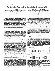
FIG. 3. Application of the iterative approach to experimental data. A sample of attenuation measurements obtained at the Scripps Pier Bubble Experiment are given in ~a! by the open circles with expected error bars. The bubble distribution as calculated by the RBA, n 0 , and the resultant attenuation, b 0 , are plotted with the dashed lines in ~b! and ~a!, respectively. The bubble distribution as calculated by the iterative approach, n t8 , and the resulting corrected attenuation, b t8 , are plotted with solid lines.

ably unwarranted in our first-order approximation.! The resulting quasicontinuous data are labeled b t , once again to imply true attenuation. For our measured-data test, we have chosen attenuation data taken during the Scripps Pier Bubble Experiment.16 The data we use here involves the average of ten measurements over 10 s and a path length of 2 m. Attenuation is measured at eight frequencies from 39 to 244 kHz. The discrete measurements, b ( f i ), and their frequencies are shown in Fig. 3~a!. Indications are that the accuracy of the measurements is near 60.1 dB/m, so a fairly close fit to these data is prescribed. The data were extrapolated to 30 kHz at the lower end and 276 kHz at the upper end, in order to fit our end measurements, and they are interpolated as discussed above. These data are then the true attenuation, b t , discussed in the previous section @not shown in Fig. 3~a!#. The iteration process alternates between the attenuation diagram @Fig. 3~a!# and the bubble-distribution diagram @Fig. 3~b!#, as was done for the simulated data. However, the figure sequence ~a!, ~b! of this figure is reversed from the simuCaruthers et al.: Bubble distributions from attenuation

188

lation sets ~Figs. 1 and 2!, because, in this case, we begin with attenuation data rather than bubble-distribution data as in the previous cases. That is, now the true distribution, n t is not known a priori in the case of real data. Given b t , the sequence of calculations ~described in the previous section! is then n 0 5RBA ~ b t ! ⇒ b 0 5FT @ n 0 # ⇒ n 80 5RBA @ b 0 # ⇒n 8t 52n 0 2n 80 , and the test of the results is the ability of b 8t 5FT @ n 8t # to match the data b ( f i ). In Fig. 3~a! we see that the RBA produces a bias of the results by up to 0.2 dB/m. In correcting the bias, we produce a match to the data within the specified accuracy of the data ~60.1 dB/m!. Note that there is a sharp rise in the distribution for bubble radii smaller than about 25 mm. This rise is quite sensitive to the attenuation data point at 244 kHz @Fig. 3~a!#; note that it appears to be somewhat high. On the other hand, that point could be real and caused by a residual population of very small bubbles. III. SUMMARY AND CONCLUSIONS

We have presented an iterative approach to inverting Eq. ~1! for application to cases where accurate attenuationversus-frequency data are known, and, correspondingly, accurate bubble-density distributions are sought. Simulated bubble distributions were used to produce a quasicontinuous set of true attenuation data by the forward evaluation of Eq. ~1!. The iterative approach was shown to produce a bubble distribution that matched the known bubble distribution better than the application of the RBA alone. As a second test of the validity of the resulting bubble distribution, the application of Eq. ~1! to this distribution produced attenuations that were a closer match to the true attenuations than a distribution calculated by the RBA. For the case of real, measured attenuation data, the true bubble distribution is not known. Therefore, only the second test can be applied. The iterative approach was applied to data taken during the Scripps Pier Bubble Experiment, and, in accordance with the second test, a bubble distribution was determined that was an improvement over the resonant bubble approximation. The accuracy of the data taken during the Scripps Pier Bubble Experiment justified the improvement provided by the iterative approach. It should be noted, however, that re-

189


sults of the approach will be to produce a distribution that will attempt to follow the data, accurate or not. The approach is suggested, therefore, only for attenuation data with sufficient accuracy to warrant its use. ACKNOWLEDGMENTS

This work is supported by the Acoustic Program of the Office of Naval Research ~ONR!. P. A. Elmore was funded by the ONR and the Naval Research Laboratory through the postdoctoral program of the American Society of Engineering Education. Physics of Sound in the Sea ~Peninsula, Los Altos, CA, 1989!, pp. 460– 477. 2 H. Medwin, ‘‘Acoustic fluctuations due to microbubbles in the nearsurface ocean,’’ J. Acoust. Soc. Am. 56, 1100–1104 ~1974!. 3 K. W. Commander and A. Prosperetti, ‘‘Linear pressure waves in bubbly liquids: Comparison between theory and experiments,’’ J. Acoust. Soc. Am. 85, 732–746 ~1989!. 4 L. M. Brekhovskikh and Y. P. Lysanov, Fundamentals of Ocean Acoustics ~Springer, Berlin, 1991!, p. 259. 5 H. Medwin, ‘‘Acoustical determinations of bubble-size spectra,’’ J. Acoust. Soc. Am. 62, 1041–1044 ~1977!. 6 K. Commander and E. Moritz, ‘‘Off-resonance contributions to acoustical bubble spectra,’’ J. Acoust. Soc. Am. 85, 2665–2669 ~1989!. 7 H. Medwin, ‘‘In situ acoustic measurements of bubble populations in coastal ocean waters,’’ J. Geophys. Res. 75, 599–611 ~1970!. 8 P. A. Kolovayev, ‘‘Investigation of the concentration and statistical size distribution of wind-produced bubbles in the near surface ocean layer,’’ Oceanology ~English Translation! 15, 659–661 ~1976!. 9 B. D. Johnson and R. C. Cooke, ‘‘Bubble populations and spectra in coastal waters: a photographic method,’’ J. Geophys. Res. 84, 3761–3766 ~1979!. 10 A. L. Walsh and P. J. Mulhearn, ‘‘Photographic measurements of bubble populations from breaking waves at sea,’’ J. Geophys. Res. 92, 14553– 14565 ~1987!. 11 H. Medwin and N. D. Breitz, ‘‘Ambient and transient bubble spectral densities in quiescent seas and under spilling breakers,’’ J. Geophys. Res. 94, 12751–12759 ~1989!. 12 S. Vagle and D. M. Farmer, ‘‘The measurements of bubble-size distributions by acoustical backscatter,’’ J. Atmos. Oceanic Tech. 9, 630–644 ~1992!. 13 H. Medwin, ‘‘In situ acoustic measurements of microbubbles at sea,’’ J. Geophys. Res. 82 No. 6, 971–976 ~1977!. 14 K. W. Commander and R. J. McDonald, ‘‘Finite-element solution to the inverse problem in bubble swarm acoustics,’’ J. Acoust. Soc. Am. 89, 592–597 ~1991!. 15 W. H. Press et al., Numerical Recipes in C: The Art of Scientific Computing, Second Edition ~Cambridge University Press, New York, 1992!, p. 134. 16 J. W. Caruthers, P. A. Elmore, S. J. Stanic, and R. R. Goodman, ‘‘The Scripps Pier Bubble Experiment of 1997,’’ Proceedings of the 16th International Congress on Acoustics and the 135th meeting of the Acoust. Soc. of Am. ~1998!, pp. 697–698. 1

Caruthers et al.: Bubble distributions from attenuation

189