sented in (Luo and Qian, 2012) and the fixed-point iteration method designed by (Waheed et al., 2014) in order to deal with high powers of spatial derivatives ...
An iterative factored eikonal solver for TTI media
B. Tavakoli F. ∗,‡ A. Ribodetti∗ , J. Virieux† , S. Operto∗ , ∗ Geoazur-CNRS-IRD-UNS-OCA; † ISTerre-UJF; ‡ Speaker
Downloaded 09/24/17 to 88.209.72.2. Redistribution subject to SEG license or copyright; see Terms of Use at http://library.seg.org/
SUMMARY Developing an accurate and efficient eikonal solver for heterogeneous tilted transversely isotropic (TTI) media is quite important for modeling, traveltime tomography or beam migration. We propose to solve the complex TTI eikonal equation through an iterative method based on the simpler elliptical anisotropic eikonal equation with a source term injecting the necessary perturbation for handling the specific TTI high-power terms. Moreover, we mitigate initial errors in describing the physical source by using a factorization method removing the point source upwind singularity. Different numerical examples on TTI models show that this strategy incorporating the iterative fixed-point procedure and the factorization method yields accurate solutions for long offsets.
INTRODUCTION Complex geological structures, like layered sediments and shale overlying salt flank, lead to mechanical anisotropy which strongly affects the seismic wave propagation. Such media can be described as vertical transversely isotropic (VTI) and tilted transversely isotropic (TTI) models. Considering the crucial role of first-arrival traveltimes computation in seismic modeling and imaging, there is a strong need for accurate and efficient methods for computing first-arrival times in VTI and TTI media. Generally traveltime computation methods are based on two ˇ main approaches: ray tracing (Cerven´ y, 2001) and wavefront tracking (Vidale, 1988). When using ray tracing, which is a lagrangian method, a rather regular sampling of the medium is difficult to achieve especially in strongly heterogeneous media. Tracking wavefronts, which is an Eulerian approach, allows a better control on the sampling of the medium and may fill also shadow zones with diffracted wavefronts when considering first-arrival times. Since the revival of an efficient finite difference approach by Vidale (1988, 1990), different improvements have been achieved when encountering high constrasts (Podvin and Lecomte, 1991), more accurate solution using the celerity domain (Pica, 1997; Zhang et al., 2005) or using an implementation of Lax-Friedrichs numerical Hamiltonian (Kao et al., 2004) to cite few contributions among many. Aside the Fast Marching Method (FMM) (see recent publication of Leli`evre et al. (2011)), the Fast Sweeping Method (FSM) has gained in popularity thanks to its highly efficient computational performance (Zhao, 2005; Noble et al., 2014) especially in heterogeneous media we encounter in the Earth. In an Eulerian frame, the eikonal equation is a non-linear partial differential equation (PDE) with boundary conditions such as the free surface and a source term which is often considered as a point singularity. As a result, the upwind source singularity introduces initial errors impacting the computation of
© 2015 SEG SEG New Orleans Annual Meeting
traveltimes. A constant velocity zone around the source point could be considered (Zhang et al., 2006; Benamou et al., 2010) which may be a problem if the source is nearby an heterogeneity. A local refinement around the source point may turn around this intrinsic problem (Kim and Cook, 1999) with subtle mesh structure for numerical implementation. Fomel et al. (2009) has proposed a rather simple and efficient method using a factorization of the traveltime as the product of an analytical known solution in a given reference medium and an unknown function to be estimated in the real medium. Inserting anisotropic rheology in the eikonal equation leads to a rather complicated non-linear PDE. Many anisotropic eikonal solvers are restricted to simple anisotropic behaviors such as the elliptical anisotropy (Qian and Symes, 2001; Luo and Qian, 2012) or may suffer from defects like heavy computational cost (Eaton, 1993) with a strong possible decrease in accuracy especially at the source (Qian et al., 2007). Therefore, a fixedpoint iterative technique has been proposed for improving the solution accuracy when considering complex anisotropic rheology while mitigating the computational cost (Alkhalifah, 2011; Ma and Alkhalifah, 2013; Waheed et al., 2014). In this study, we combine the factorized eikonal equation presented in (Luo and Qian, 2012) and the fixed-point iteration method designed by (Waheed et al., 2014) in order to deal with high powers of spatial derivatives existing in the eikonal equation in TTI media. We propose to develop a new fast eikonal anisotropic solver that removes source singularity and computes accurately first-arrival traveltime in complex TTI media. We first describe the method before an illustration of its efficiency and accuracy for both far and near offsets through examples for homogeneous VTI/TTI, heterogeneous TTI and BP TTI salt model. METHOD The eikonal equation for TTI media have components with products of power greater than two of first-order spatial derivatives leading to numerical difficulties for precise solutions when the first derivative is discretized. We shall proceed through an iterative procedure for mitigating these errors. Fixed-point iteration technique Following Alkhalifah (2003); Waheed et al. (2014), in 2D heterogeneous TTI media, the 2D eikonal equation can be written as follows 2 d 2 d 2 d 2 A(∂d (1) x T ) +C(∂z T ) + E(∂x T ) (∂z T ) = 1, where
∂d x T = ∂x T cos θ − ∂z T sin θ , ∂d z T = ∂x T sin θ + ∂z T cos θ ,
(2)
are the spatial derivatives of the traveltime function T (x, z) in the local rotated coordinate system defined for TTI tilted an-
DOI http://dx.doi.org/10.1190/segam2015-5863984.1 Page 3576
TTI factored eikonal solver
Downloaded 09/24/17 to 88.209.72.2. Redistribution subject to SEG license or copyright; see Terms of Use at http://library.seg.org/
gle θ . Coefficient A,C, E are defined locally through relations A = v2nmo (1+2η),C = v20 , and E = −2ηv2nmo v20 , where the vertical velocity is denoted by v0 and the normal moveout velocity by vnmo . The anelliptic anisotropic parameter is given by the expression η = (ε − δ )/(1 + 2δ ) (Thomsen, 1986; Tsvankin, 1997). By inserting equations (2) into the equation (1), we end up with the equation a0 (∂x T )2 − 2c0 (∂x T )(∂z T ) + b0 (∂z T )2 = H(T ),
(3)
a0 = A cos2 θ +C sin2 θ , b0 = A sin2 θ +C cos2 θ , c0 = (A −C) cos θ sin θ ,
(4)
where
and the right-hand-side term H(T ), defined as 1 − E (∂x T cos θ − ∂z T sin θ )2 (∂x T sin θ + ∂z T cos θ )2 , (5) includes all products with higher powers than two of traveltime derivatives introduced by the TTI behavior. The left-hand-side term is very similar to the one we have in the equation for elliptical anisotropy as underlined by Luo and Qian (2012) which can be written as q a(x)(∂x T )2 − 2c(x)(∂x T )(∂z T ) + b(x)(∂z T )2 = 1 (6)
which will be solved by FSM in our case. To cope with these high-order terms in the equation (3), Waheed et al. (2014) suggested to proceed iteratively through a fixed-point method (Kelley, 1995) where the eikonal equation (3) is reformulated as a0 (∂x Tn )2 − 2c0 (∂x Tn )(∂z Tn ) + b0 (∂z Tn )2 = H(Tn−1 ),
(7)
medium and will correct the traveltime estimation when considering heterogeneities. As a result, the gradient of traveltime can be expressed through following compact expressions ∂x T ≡ Tx = T0x τ + τx T0 , ∂z T ≡ Tz = T0z τ + τz T0 ,
(11)
with obvious notations for derivatives. By inserting equation (11) into the equation (6), we obtain the factorized anisotropic eikonal equation (Luo and Qian, 2012), s τ 2 (aT02x − 2cT0x T0z + bT02z ) + 2T0 τ(aT0x τx = 1. −c(Tox τz + T0z τx ) + bT0z τz ) + T02 (aτx2 − 2cτx τz + bτz2 ) (12) The quantity T0 should capture the source singularity and, therefore, the quantity τ should be a rather smooth function around the source. In an homogeneous medium, the quantity T0 can be computed analytically through the expression s b0 (x − x0 )2 + 2c0 (x − x0 )(z − z0 ) + a0 (y − y0 )2 , T0 (x, z) = a0 b0 − c20 (13) as well as its spatial derivatives. Coefficients a0 = a(x0 ), b0 = b(x0 ) and c0 = c(x0 ) are those at the source. Luo and Qian (2012) proposed a first-order FSM on rectangular meshes as a promising method to compute numerically τ in equation (12). They considered a rectangular mesh with grid size h and discretize equation (12) thorough four triangles (Fig.1). This discretization provides an upwind scheme respecting causality condition for the fast sweeping method. For example, a discretization through the triangle 4WCN for
and n ≥ 1 indicates the fixed-point iteration number. By taking advantage of this iterative method, we introduce the following quantities an →
b0 c0 a0 , bn → , cn → H(Tn ) H(Tn ) H(Tn )
(8)
and rewrite the equation (6) for the iteration n of a fixed-point loop as follows: q an−1 (∂x Tn )2 + bn−1 (∂z Tn )2 − 2cn−1 (∂x Tn )(∂z Tn ) = 1. (9) Solving this eikonal equation yields Tn (x) which enables us to update new coeffficients an , bn , cn and to restart the procedure for a new estimation of the traveltime until convergence. We considered H(T0 ) = 1 as the initial guess to build initial coefficients a0 , b0 , c0 . In our applications, we have limited the maximum number of iterations to 10 and sometimes the convergence to a relative precision of 10−9 is obtained faster. Factorized eikonal solver According to the factorization method (Fomel et al., 2009), the solution of equation (9) can be decomposed into the product T = T0 τ,
SEG New Orleans Annual Meeting
vertex C can be applied by a linear Taylor expansion of τx and τz through expressions � � τ(C) − τ(W ) τ(C) − τ(S) (τx (C), τz (C)) ≈ , . (14) h h
By inserting equation (14) into the factorized anisotropic eikonal equation (12), we reach the following discretized eikonal equation q k1 τ 2 (C) + k2 τ(C) + k3 = 1, (15) where we define three new quantities as k1
= +
(10)
where T0 is a known analytical solution of a simple eikonal equation in an homogeneous medium with the velocity at the source. The quantity τ should be computed at each point of the
© 2015 SEG
Figure 1: Rectangular mesh and neighbor grid points for central vertex C, (from Luo and Qian, 2012).
k2
= −
aT0x 2 − 2cT0x T0z + bT0z 2 + 2
T0 (T0x (a − c) + T0z (b − c)) h
T02 (a − 2c + b), h2 T0 2 (τ(W )(cT0z − aT0x ) + τ(S)(cT0x − bT0z )) h T02 2 2 (aτ(W ) − c(τ(W ) + τ(S)) + bτ(S)), h
DOI http://dx.doi.org/10.1190/segam2015-5863984.1 Page 3577
TTI factored eikonal solver T02 (aτ 2 (W ) − 2cτ(W )τ(S) + bτ 2 (S)). h2 So given the neighbours values, τ(W ) and τ(S), for triangle 4WCN, a quadratic equation solver can compute the value of τ h (C), where the grid size is denoted by h. For the other triangles, this discretization results also in a quadratic equation. The acceptable solutions for τ(C) need to be real and satisfy the causality condition. We recall the causality condition as follows: the characteristic of function T passing through vertex C of each triangle should be between to the edges of triangle, (Fig. 1). For instance, for the triangle 4WCN the characteristic vector passing C is defined as
Downloaded 09/24/17 to 88.209.72.2. Redistribution subject to SEG license or copyright; see Terms of Use at http://library.seg.org/
k3 =
(a(C)Txh (C) − c(C)Tzh (C), b(C)Tzh (C) − c(C)Txh (C)). (16) In order to satisfy the causality condition, it should be be−→ − → tween edges WC and SC. Here ∇T h (C) = ∇τ h (C)T0 (C) + h τ (C)∇T0 (C). When equation (15) yields no real solution for τ h (C), we can convey information about τ from neighbours to center vertex C along the edges of triangle and compute a viscosity solution for τ h (C) through the method of characteristics. This solution for the triangle 4WCN is given by q b(C) T0 (C)τ(W ) + h a(C)b(C)−c2 (C) h τ (C) = (17) T0 (C) + T0x (C)(xC − xW ) as proposed by Luo and Qian (2012). Each of the four triangles defining a FD scheme can provide center vertex with several candidates all satisfying the causality condition: only the minimum one will be selected by FSM. In other words, for each grid point, the FSM calculates traveltimes for four different sweeps and in each sweep, the factorization method finds one candidate for traveltime. So, each sweep presents a value for travel time that the minimum value is considered as the solution. Of course, we have to repeat the procedure for the next iteration. NUMERICAL EXAMPLES In this section, we assess the accuracy of our eikonal solver with different numerical examples involving long-distance propagation. These tests consider homogeneous isotropic and VTI models, as references, and three TTI models: homogeneous medium, constant-velocity gradient model and a complex model, the BP salt model (Shah, 2007). For all the examples the grid step h has a value of 50 meters. Homogeneous media Isotropic model: The dimensions of the subsurface model are 20000 m × 4000 m with a P-wavespeed Vp = 3 km/s. The source is located at the upper-left corner of the computational grid. The solution of the eikonal solver is validated against the analytical solution (Fig. 2a). The difference map shows that eikonal solver accurately accounts for the point source singularity. The maximum error between numerical and analytical solutions is less than 0.25 %. VTI model: For this model, physical parameters are the following ones: Vp = 3 km/s, ε = 0.15, δ = 0.05 and x0 = z0 = 0 m. We compare the analytical solution of Carcione et al. (1988)
© 2015 SEG SEG New Orleans Annual Meeting
with the numerical solution. Figure 2b shows different wavefronts and, the precision we reach is similar to the isotropic case, which is an acceptable accuracy range for different applications. TTI models We validate the eikonal solver we have developed against full wavefield solutions computed with a O(∆t 2 , ∆x4 ) TTI acoustic finite-difference time-domain (FDTD) code based on the staggered-grid stencil of Saenger et al. (2000) and the SMART absorbing boundary conditions of M´etivier et al. (2014). For a homogeneous TTI model (Vp = 3.5 km/s, θ = 30◦ , ε = 0.15, δ = 0.05) traveltime error increases with offsets as illustrated in the Figure 3a. A strong clipping on the wavefield has been performed on the snapshot in order to see the first-arrival phase matching the traveltime computation. Parasite phases coming from absorbing boundary layers are now visible in the snapshot but not in the traveltime curve. For constant gradient velocity TTI model (Vp = 2 − 3.9 km/s, θ = 30◦ , ε = 0.15, δ = 0.05), we can see that errors at large offsets are less than in the previous case, thanks to the wavefront curvature (Fig. 3b). For BP salt model, the wavefront curvature is significant and, therefore, the value of error for τ stays relatively small: an error of approximatively ≈ 1.5% is observed where waves passe through high-velocity salt before reaching the surface (Fig. 3c). Results indicate the high accuracy and precision of the eikonal solver we have developed in the estimation of first arrivals even for far offsets, (Table 1). CONCLUSIONS We have presented an iterative factorized eikonal solver for heterogeneous TTI media. The strategy is based on a fixed point iterative solver: the simpler elliptical anisotropic eikonal equation is solved by a fast sweeping method with updated right-hand-side terms for converging toward the TTI solution. Adding the factorization procedure removes the singularity at the source and improves dramatically the precision of the solution. Examples of complex geological TTI models point out the ability of this method for a precise estimation of firstarrival times for near and far offsets. We have identified convergence difficulties of modifying the assumed analytical solution at far offsets where wavefronts tend to be planar. Nethertheless, the method is enough accurate to consider it for traveltime tomography and anisotropic stereotomography. ACKNOWLEDGEMENTS This study was partially funded by the sponsors of the SEISCOPE consortium (/http://seiscope2.osug.fr). This study was granted access to the HPC resources of SIGAMM and CIMENT computer centers and CINES/IDRIS under the allocation 046091 made by GENCI. We thank L. M´etivier (LJK/CNRS) for providing us his TTI finite-difference modeling code and for interesting discussions.
DOI http://dx.doi.org/10.1190/segam2015-5863984.1 Page 3578
TTI factored eikonal solver
Downloaded 09/24/17 to 88.209.72.2. Redistribution subject to SEG license or copyright; see Terms of Use at http://library.seg.org/
a)
b)
Figure 2: (a) Difference between analytical and numerical solution in percentage for homogeneous isotropic model. (b) Superimposition of traveltime contours at times 0.64s, 2.4s and 4.8s, calculated by analytical solution(green) and eikonal solver (red) for homogeneous VTI model.
Figure 3: Numerical examples. (a) Homogeneous medium. Top four panels: Traveltime contours (red line) superimposed on the FDTD wavefield at times 2s, 3s, 5s and 7s with a strong saturation showing parasite phases from borders. Bottom panel: Traveltimes computed with the eikonal solver (red line) superimposed on the FDTD seismograms without saturation. The receiver line is at 200m depth. (b) Same as (a) for a velocity gradient model. (c) TTI BP salt model. Top four panels: Traveltime contours (red line) superimposed on the FDTD wavefield at times 2s, 3s, 6s and 10s with a reduced saturation. Bottom panel: Traveltimes computed with the eikonal solver (red line) superimposed on the FDTD seismograms. Model H-TTI CG-TTI
1 0.05% 0.05%
3 0.1% 0.1%
5 0.4% 0.4%
7 0.55% 0.55%
9 0.8% 0.5%
Distance(km) 12 15 1% 1.1% 0.4% 0.35%
18 1.2% 0.3%
21 1.25% 0.2 %
24 1.27% 0.3 %
27 1.27% 0.5 %
Table 1: Error estimation according to distances for homogeneous TTI (H-TTI) and constant gradient velocity TTI (CG-TTI) models when considering this new eikonal solver.
© 2015 SEG SEG New Orleans Annual Meeting
DOI http://dx.doi.org/10.1190/segam2015-5863984.1 Page 3579
EDITED REFERENCES Note: This reference list is a copyedited version of the reference list submitted by the author. Reference lists for the 2015 SEG Technical Program Expanded Abstracts have been copyedited so that references provided with the online metadata for each paper will achieve a high degree of linking to cited sources that appear on the Web.
Downloaded 09/24/17 to 88.209.72.2. Redistribution subject to SEG license or copyright; see Terms of Use at http://library.seg.org/
REFERENCES
Alkhalifah, T., 2003, An acoustic wave equation for orthorhombic anisotropy: Geophysics, 68, 1169–1172, http://dx.doi.org/10.1190/1.1598109. Alkhalifah, T., 2011, Scanning anisotropy parameters in complex media: Geophysics, 76, no. 2, U13–U22, http://dx.doi.org/10.1190/1.3553015. Benamou, J. D., S. Luo, and H.-K. Zhao, 2010, A compact upwind second order scheme for the eikonal equation: Journal of Computational Mathematics, 28, no. 4, 489–516, doi:10.4208/jcm.1003-m0014. Carcione, J. M., D. Kosloff, and R. Kosloff, 1988, Wave-propagation simulation in an elastic anisotropic (transversely isotropic) solid: The Quarterly Journal of Mechanics and Applied Mathematics, 41, no. 3, 319–346, http://dx.doi.org/10.1093/qjmam/41.3.319. Červený, V., 2001, Seismic ray theory: Cambridge University Press, http://dx.doi.org/10.1017/CBO9780511529399. Eaton, D., 1993, Finite difference traveltime calculation for anisotropic media: Geophysical Journal International, 114, no. 2, 273–280, http://dx.doi.org/10.1111/j.1365246X.1993.tb03915.x. Fomel, S., S. Luo, and H.-K. Zhao, 2009, Fast sweeping method for the factored eikonal equation: Journal of Computational Physics, 228, no. 17, 6440– 6455, http://dx.doi.org/10.1016/j.jcp.2009.05.029. Kao, C. Y., S. Osher, and J. Qian, 2004, Lax-Friedrichs sweeping schemes for static HamiltonJacobi equations: Journal of Computational Physics, 196, no. 1, 367– 391, http://dx.doi.org/10.1016/j.jcp.2003.11.007. Kelley, C., 1995, Iterative methods for linear and nonlinear equations: SIAM, http://dx.doi.org/10.1137/1.9781611970944. Kim, S., and R. Cook, 1999, 3-D traveltime computation using second order ENO scheme: Geophysics, 64, 1867–1876, http://dx.doi.org/10.1190/1.1444693. Lelièvre, P. G., C. G. Farquharson, and C. A. Hurich, 2011, Computing first-arrival seismic traveltimes on unstructured 3-D tetrahedral grids using the fast marching method: Geophysical Journal International, 184, no. 2, 885–896, http://dx.doi.org/10.1111/j.1365246X.2010.04880.x. Luo, S., and J. Qian, 2012, Fast sweeping method for factored anisotropic eikonal equations: Multipicative and additive factors: Journal of Scientific Computing, 52, no. 2, 360– 382, http://dx.doi.org/10.1007/s10915-011-9550-y. Ma, X., and T. Alkhalifah, 2013, q-P wave traveltime computation by an iterative approach: 75th Conference & Exhibition, EAGE, Extended Abstracts, doi:10.3997/2214-4609.20130722. Métivier, L., R. Brossier, S. Labbe, S. Operto, and J. Virieux, 2014, A robust absorbing layer method for anisotropic seismic wave modeling: Journal of Computational Physics, 279, 218– 240, http://dx.doi.org/10.1016/j.jcp.2014.09.007.
© 2015 SEG SEG New Orleans Annual Meeting
DOI http://dx.doi.org/10.1190/segam2015-5863984.1 Page 3580
Noble, M., A. Gesret, and N. Belayouni, 2014, Accurate 3-D finite difference computation of travel time in strongly heterogeneous media: Geophysical Journal International, 199, no. 3, 1572–1585, http://dx.doi.org/10.1093/gji/ggu358. Downloaded 09/24/17 to 88.209.72.2. Redistribution subject to SEG license or copyright; see Terms of Use at http://library.seg.org/
Pica, A., 1997, Fast and accurate finite difference solution of the 3D eikonal equation parameterized in celerity: 67th Annual International Meeting, SEG, Expanded Abstracts, 1774–1777. Podvin, P., and I. Lecomte, 1991, Finite difference computation of traveltimes in very contrasted velocity model: A massively parallel approach and its associated tools: Geophysical Journal International, 105, no. 1, 271–284, http://dx.doi.org/10.1111/j.1365-246X.1991.tb03461.x. Qian, J., and W. W. Symes, 2001, Paraxial eikonal solvers for anisotropic quasi-P travel times: Journal of Computational Physics, 173, no. 1, 256– 278, http://dx.doi.org/10.1006/jcph.2001.6875. Qian, J., Y.-T. Zhang, and H.-K. Zhao, 2007, A fast sweeping method for static convex Hamilton–Jacobi equations: Journal of Scientific Computing, 31, no. 1-2, 237– 271, http://dx.doi.org/10.1007/s10915-006-9124-6. Saenger, E. H., N. Gold, and S. A. Shapiro, 2000, Modeling the propagation of elastic waves using a modified finite-difference grid: Wave Motion, 31, no. 1, 77– 92, http://dx.doi.org/10.1016/S0165-2125(99)00023-2. Shah, H., 2007, The 2007 BP anisotropic velocity-analysis benchmark: Presented at the 70th Conference & Exhibition Workshop, EAGE. Thomsen, L. A., 1986, Weak elastic anisotropy: Geophysics, 51, 1954– 1966, http://dx.doi.org/10.1190/1.1442051. Tsvankin, I., 1997, Anisotropic parameters and P-wave velocity for orthorhombic media: Geophysics, 62, 1292–1309, http://dx.doi.org/10.1190/1.1444231. Vidale, D., 1988, Finite-difference calculation of travel time: Bulletin of the Seismological Society of America, 78, no. 6, 2062–2076. Vidale, J., 1990, Finite-difference calculation of traveltimes in three dimensions: Geophysics, 55, 521–526, http://dx.doi.org/10.1190/1.1442863. Waheed, U. B., C. E. Yarman, and G. Flagg, 2014, An iterative fast sweeping based eikonal solver for tilted orthorhombic media: 84th Annual International Meeting, SEG, Expanded Abstracts, 480–485. Zhang, L., J. W. Rector III, and G. M. Hoversten, 2005, Eikonal solver in the celerity domain: Geophysical Journal International, 162, no. 1, 1–8, http://dx.doi.org/10.1111/j.1365246X.2005.02626.x. Zhang, Y.-T., H.-K. Zhao, and J. Qian, 2006, High order fast sweeping methods for static Hamilton–Jacobi equations: Journal of Scientific Computing, 29, no. 1, 25– 56, http://dx.doi.org/10.1007/s10915-005-9014-3. Zhao, H., 2005, A fast sweeping method for eikonal equations: Mathematics of Computation, 74, 603–627, http://dx.doi.org/10.1090/S0025-5718-04-01678-3.
© 2015 SEG SEG New Orleans Annual Meeting
DOI http://dx.doi.org/10.1190/segam2015-5863984.1 Page 3581