An MDL framework for sparse coding and dictionary learning - arXiv

1

An MDL framework for sparse coding and dictionary learning Ignacio Ram´ırez and Guillermo Sapiro

arXiv:1110.2436v1 [cs.IT] 11 Oct 2011

Abstract The power of sparse signal modeling with learned over-complete dictionaries has been demonstrated in a variety of applications and fields, from signal processing to statistical inference and machine learning. However, the statistical properties of these models, such as under-fitting or over-fitting given sets of data, are still not well characterized in the literature. As a result, the success of sparse modeling depends on hand-tuning critical parameters for each data and application. This work aims at addressing this by providing a practical and objective characterization of sparse models by means of the Minimum Description Length (MDL) principle – a well established informationtheoretic approach to model selection in statistical inference. The resulting framework derives a family of efficient sparse coding and dictionary learning algorithms which, by virtue of the MDL principle, are completely parameter free. Furthermore, such framework allows to incorporate additional prior information to existing models, such as Markovian dependencies, or to define completely new problem formulations, including in the matrix analysis area, in a natural way. These virtues will be demonstrated with parameter-free algorithms for the classic image denoising and classification problems, and for low-rank matrix recovery in video applications. Index Terms Sparse coding, dictionary learning, MDL, denoising, classification, low-rank matrix completion.

I. I NTRODUCTION A sparse model is one in which signals of a given type y ∈ Rm can be represented accurately as sparse linear combinations of the columns (atoms) of a learned dictionary D ∈ Rm×p , y = Da + e, where by accurate we mean that kek  kyk (in some norm), and by sparse we mean that the number of non-zero elements in a, denoted by kak0 , is small compared to its dimension p. These concepts will be formalized in the next section. Such models, especially when D is learned from training samples, are by now a well established tool in a variety of fields and applications, see [1], [2], [3] for recent reviews. When sparsity is a modeling device and not an hypothesis about the nature of the analyzed signals, parameters such as the desired sparsity in the solutions, or the size p of the dictionaries to be learned, play a critical role in the effectiveness of sparse models for the data and tasks at hand. However, lacking theoretical guidelines for such parameters, published applications based on learned sparse models often rely on either cross-validation or ad-hoc methods for determining such critical parameters (an exception for example being the Bayesian approach, e.g., [4]). Clearly, such techniques can be impractical and/or ineffective in many cases. This in turn hinders the further application of such models to new types of data and applications, or their evolution into different, possibly more sophisticated, models. At the bottom of the aforementioned problem lie fundamental questions such as: How rich or complex is a sparse model? How does this depend on the required sparsity of the solutions, or the size of the dictionaries? What is the best model for a given data class and a given task? The general problem of answering such questions and, in particular, the latter, is known as model selection. Popular model selection techniques such as Akaike’s Information Criterion (AIC) [5], Bayes Information Criterion (BIC) [6], and the Minimum Description Length principle (MDL) [7], [8], [9], work by building a cost function which balances a measure of goodness of fit with one of model complexity, and search for a model that minimizes such cost. In this sense, these tools can be regarded as practical implementations of the Occam’s razor principle, which states that, given two (equally accurate) descriptions for a given phenomenon, the simpler one is usually the best. Department of Electrical and Computer Engineering, University of Minnesota. Work supported by NSF, NGA, ARO, ONR, DARPA and NSSEFF.

2

In the Minimum Description Length principle, given a family or model class M of candidate models indexed by ˆ ∈ M is the one that can be used to describe y completely a parameter M , and a data sample y, the best model M (including the parameters M themselves) with the fewest number of bits, ˆ = arg min L(y, M ), M M ∈M

(1)

where L(y, M ) is a codelength assignment function which defines the theoretical codelength required to describe (y, M ) uniquely, and which is a key component of any MDL-based framework. The underlying idea of MDL is that compressibility is a good indirect way of measuring the ability of a model to capture regularity from the data. Common practice in MDL uses the Ideal Shannon Codelength Assignment [10, Chapter 5] to define L(y, M ) in terms of a probability assignment P(y, M ) as L(y, M ) = − log P(y, M ) (all logarithms will be assumed on base 2 hereafter). In this way, the problem of choosing L(·) becomes one of choosing a suitable probability model for (y, M ). Note here how MDL considers probability models not as a statement about the true nature of the data, but only as a modeling tool. If we now write P(y, M ) = P(y|M )P(M ), we obtain the more familiar penalized likelihood form, ˆ = arg min − log P(y|M ) − log P(M ), M (2) M ∈M

with − log P(M ) representing the model complexity, or model cost, term. The use of MDL for sparse signal modeling has been explored for example in the context of wavelet-based denoising (where M = a ∈ Rm , p = m and D ∈ Rm×m is fixed) of images corrupted by additive white Gaussian noise (AWGN) [11], [12], [13], [14], [15]. In [11], [12], [13], the data is described using (2) with − log P(y|a) assumed to be solely due to noise, and an L(a) term which exploits sparsity, ˆ = arg min a

a∈M

1 ky − Dak22 + L(a). 2 2σe

(3)

Here the first term corresponds to the ideal codelength, up to a constant, of an IID Gaussian sequence of zero mean and known variance σe2 . The difference between [11], [12], [13] lies in the definition of L(a). The line of work [14], [15] follows the modern MDL approach by using sophisticated tools from coding theory, the so called one-part universal codes, which encodes (y, a) jointly, and reduces the arbitrariness in defining L(a). However, such tools can only be applied for certain choices of P(y|a) and P(a). In the case of [14], [15], the choice is to use continuous Gaussian models for both. As Gaussian models are not well suited to the typically observed statistical properties of such data, the performance of the resulting denoisers for example is very poor compared to the current state-of-the-art. The present work extends and/or improves on the aforementioned work in the following ways:1 • MDL-based sparse coding is extended to the case of non-orthonormal, possibly over-complete and learned dictionaries D. As we will see in Section V, this extension, critical to deal with modern, very successful sparse modeling approaches, poses not only new design problems but also significant computational challenges compared to the orthonormal case. • Efficient codelengths (probability distributions) for the different components to encode (error, coefficients, dictionary) are obtained by applying universal coding schemes to priors that are suited to the typically observed statistics of such data. • As a particular point of the above item, systematic model-fit deviations are naturally taken into account in P(y|a). The resulting fitting terms fall into the category of robust estimators (see [17]), thus marrying robust statistics with information theory and with sparse modeling (dictionary learning). • We comply with the basic MDL sanity check, meaning, that the theoretical codelengths obtained are smaller than a “raw” description of the data. We do so by including quantization in our models, and treating its effect rigorously. • Dictionary learning within the MDL framework allows us to optimize both the number of atoms p, as well as their structure, resulting in a natural and objective form of regularization for D. 1 This paper extends preliminary results reported in [16]. In particular, new dictionary learning algorithms are developed which include `1 atom regularization, forward and backward dictionary size adaptation. We also develop a new model for the low-rank matrix approximation problem.

3

Structure is naturally added to the sparse models in the form of Markovian dependencies between adjacent data samples. We also show an extension of the model to the problem of low-rank matrix completion. As a result of the above features, we obtain for the first time an MDL-based, parameter-free framework for signal modeling that is able to yield state-of-the-art results. At the theoretical level, this brings us a step closer to the fundamental understanding of learned sparse models and brings a different perspective, that of MDL, into the sparse modeling world. The remainder of this paper is organized as follows. Sparse models, and the associated notation, are described in detail in Section II. Section III introduces MDL, and its application to sparse models. In Section IV we present the probability models used to assign codelengths to different parts of the encoded data, while sections V and VI describe the actual sparse coding and dictionary learning algorithms developed. Experimental results follow in Section VII, and the paper is concluded in Section VIII. •

II. BACKGROUND ON SPARSE MODELING Assume we are given n m-dimensional data samples ordered as columns of a matrix Y = [y1 |y2 | . . . |yn ] ∈ Consider a linear model for Y, Y = DA + E, where D = [d1 |d2 | . . . |dp ] is an m×p dictionary consisting of p atoms, A = [a1 |a2 | . . . |an ] ∈ Rp×n is a matrix of coefficients where each j -th column aj specifies the linear combination of columns of D that approximates yj , and E = [e1 |e2 | . . . |en ] ∈ Rm×n is a matrix of approximation errors. We define the support, or active set, of a vector a ∈ Rp as supp(a) = {k : ak 6= 0}. Let Γ = supp(a). We also represent the support of a as a binary vector z ∈ {0, 1}p such that zi = 1 for i ∈ Γ, and 0 otherwise. We refer to the sub-vector in R|Γ| of non-zero elements of a as either a[Γ] or a[z] . Both conventions are extended to refer to sets of columns of matrices, for example, P D[Γ] is the matrix formed by the |Γ| columns of D indexed by Γ. We will use the pseudo-norm kak0 := |Γ| = z to denote the number of non-zero elements of a. We say that the model is sparse if we can achieve kej k2  kyj k2 and kak0  p simultaneously for all or most j = 1, . . . , n. The result of quantizing a real-valued variable y to precision δ is denoted by [y]δ . This notation is extended to denote element-wise quantization of vector (e.g., [e]) and matrix operands (e.g., [E]). Rm×n .

A. Sparse coding One possible form of expressing the sparse coding problem is given by ˆj = arg minp kyj −Duk2 a u∈R

s.t.

kuk0 ≤ γ,

(4)

where γ  p indicates the desired sparsity level of the solution. Since problem (4) is non-convex and NP-hard, approximate solutions are sought. This is done either by using greedy methods such as Matching Pursuit (MP) [18], or by solving a convex approximation to (4), commonly known as the lasso [19], 1 kyj − Duk2 s.t. kuk1 ≤ τ. (5) u∈R 2 There exists a body of results showing that, under certain conditions on γ and D, the problem (4) can be solved exactly via (5) or MP (see for example [1], [20]). In other cases, the objective is not to solve (4), but to guarantee ˆj . For example, in the above mentioned case of AWGN denoising in the wavelets some property of the estimated a domain, the parameter τ can be chosen so that the resulting estimators are universally optimal with respect to some class of signals [21]. However, if D is arbitrary, no such choice exists. Also, if D is orthonormal, the problem (5) admits a closed form solution obtained via the so-called soft thresholding [21]. However, again, for general D, no such solution exists, and the search for efficient algorithms has been a hot topic recently, e.g., [22], [23], [24]. ˆj = arg minp a

B. Dictionary learning When D is an optimization variable, we refer to the resulting problem as dictionary learning: ˆ D) ˆ = arg min (A, A,D

n X 1 j=1

2

kyj − Daj k22

s.t.

kaj kr ≤ τ ∀ j, kdk k2 ≤ 1 ∀k,

(6)

4

with 0 ≤ r ≤ 1. The constraint kdk k2 ≤ 1 , k = 1, . . . , p, is necessary to avoid an arbitrary decrease of the cost function by setting D ← αD, A ← α1 A, for any α > 1. The cost function in (6) is non-convex in (A, D), so that only local convergence can be guaranteed. This is usually achieved using alternate optimization in D and A. See for example [25], [26] and references therein. C. Issues with traditional sparse models: a motivating example Consider the K-SVD-based [25] sparse image restoration framework [27]. This is an `0 -based dictionary learning framework, which approximates (6) for the case r = 0 by alternate minimization. In the case of image denoising, the general procedure can be summarized as follows: 1) An initial, global dictionary D0 is learned using training samples for the class of data to be processed (in this case small patches of natural images). The user must supply a patch width w, a dictionary size p and a value for τ . 2) The noisy image is decomposed into overlapping w×w patches (one patch per pixel of the image), and its noisy patches are used to further adapt D using the following denoising variant of (6), ˆ A) ˆ = arg min (D, D,A

n X j=1

kaj k0 ,

s.t.

1 kyj − Daj k22 ≤ Cσ 2 , 2

kdk k2 = 1 , k = 1, . . . , p.

(7)

Here the user must further supply a constant C (in [27], it is 1.32), the noise variance σ 2 , and the number of iterations J of the optimization algorithm, which is usually kept small to avoid over-fitting (the algorithm is not allowed to converge). ˆ =D ˆA ˆ into the corresponding original positions 3) The final image is constructed by assembling the patches in Y of the image. The final pixel value at each location is an average of all the patches to which it belongs, plus a small fraction 0 ≤ λ ≤ 1 of the original noisy pixels (λ = 30/σ in [27]). Despite the good results obtained for natural images, several aspects of this method are not satisfactory: • Several parameters (w , p, τ , C , J , λ) need to be tuned. There is no interpretation, and therefore no justifiable choice for these parameters, other than maximizing the empirical performance of the algorithm (according to some metric, in this case PSNR) for the data at hand. • The effect of such parameters on the result is shadowed by the effects of later stages of the algorithm and their associated parameters (e.g. overlapping patch averaging). There is no fundamental way to optimize each stage separately. As a partial remedy to the first problem, Bayesian sparse models were developed (e.g., [4]) where these parameters are assigned prior distributions which are then learned from the data. However, this approach still does not provide objective means to compare different models (with different priors, for example). Further, the Bayesian technique implies having to repeatedly solve possibly costly optimization problems, increasing the computational burden of the application. As mentioned in the introduction, this work proposes to address the above practical issues, as well as to provide a new angle into dictionary learning, by means of the MDL principle for model selection. The details on how this is done are the subject of the following sections. III. S PARSE MODEL SELECTION AND MDL Given data Y, a maximum support size γ and a dictionary size p, traditional sparse modeling provides means to estimate the best model M = (A, D) for Y within the set M(γ, p) defined as  M(γ, p) := (A, D) : kaj k0 ≤ γ, j = 1, . . . , n, D ∈ Rm×p . (8) We call such set a sparse model class with hyper-parameters (γ, p). Such classes are nested in the following way: first, for a fixed dictionary size p we have M(γ − 1, p) ⊂ M(γ, p). Also, for fixed γ , if we consider M(γ, p − 1) to be a particular case of M(γ, p) where the p-th atom is all-zeroes and apj = 0, ∀j , then we also have that M(γ, p − 1) ⊂ M(γ, p). If one wants to choose the best model among all possible classes M(γ, p), the problem becomes one of model selection. The general objective of model selection tools is to define an objective criterion for choosing such model.

5

In particular, MDL model selection uses codelength as such criterion. More specifically, this means first computing the best model within each family as (A(γ, p), D(γ, p)) = arg min{L(Y, A, D) : (A, D) ∈ M(γ, p)},

and then choosing (ˆ γ , pˆ) = arg min {L(Y, A(γ, p), D(γ, p)) : 0 ≤ γ ≤ p, p > 0}. When D is fixed,  which is the case of sparse coding, the only model parameter is A, and we have p + 1 possible classes, M(γ) = A : kaj k0 ≤ γ, j = 1, . . . , n , one for each 0 ≤ γ ≤ p. If each data sample yj from Y is encoded independently, then, as with traditional sparse coding (the framework can also be extended to collaborative models), the model selection problem can be broken into n sub-problems, one per sample, by redefining the model class accordingly as M(γ) = {a : kak0 ≤ γ}. Clearly, in the latter case, the optimum γ can vary from sample to sample. Compared to the algorithm in Section II-C, we have a fundamental, intrinsic measure of the quality of each model, the codelength L(Y, A, D), to guide our search through the models, and which is unobscured from the effect of possible later stages of the application. In contrast, there is no obvious intrinsic measure of quality for models learned through (8), making comparisons between models learned for different parameters (patch width w, regularization parameter τ , norm r, constants C, λ) possible only in terms of the observed results of the applications where they are embedded. The second advantage of this framework is that it allows to select, in a fundamental fashion, the best model parameters automatically, thus resulting in parameter-free algorithms.2 Such advantages will be of practical use only if the resulting computational algorithms are not orders of magnitude slower than the traditional ones, and efficient algorithms are a critical component of this framework, see Section V. A. A brief introduction to MDL For clarity of the presentation, in this section we will consider D fixed, and a single data sample y to be encoded. The Minimum Description Length principle was pioneered by Rissanen [7] in what is called “early MDL,” and later refined by himself [8] and other authors to form what is today known as “modern MDL” (see [28] for an up-to-date extensive reference on the subject). The goal of MDL is to provide an objective criterion to select the model M , out of a family of competing models M, that gives the best description of the given data y. In this case of sparse coding with fixed dictionary we have M = a. The main idea of MDL is that, the best model for the data at hand is the one that is able to capture more regularity from it. The more regularity a model captures, the more succinct the description of the data will be under that model (by avoiding redundancy in the description). Therefore, MDL will select the best model as the one that produces the shortest (most efficient) description of the data, which in our case is given by L(y, a). As mentioned in Section I, MDL translates the problem of choosing a codelength function L(·) to one of choosing probability models by means of the ideal Shannon codelength assignment L(y, a) = − log P(y, a). It is common to extend such ideal codelength to continuous random variables x with probability density function p(x) as L(x) = − log p(x), by assuming that they will be quantized with sufficient precision so that P([x]δ ) ≈ p(x)δ,

(9)

and disregarding the constant term − log δ in L(x), as it is inconsequential for model selection. However, in our framework, the optimum quantization levels will often be large enough so that such approximations are no longer valid. ˆ used to encode y need to be To produce a complete description of the data y, the best model parameters M ˆ belongs to a given class M, then the cost included in the description as well. If the only thing we know is that M of this description will depend on how large and complex M is. MDL will penalize more those models that come from larger (more complex) classes. This is summarized in one of the fundamental results underlying MDL [8], which establishes that the minimum number of bits required for encoding any data vector y using a model from a class M has the form LM (y) = LM (y) + C(M), where LM (y) is called the stochastic complexity, which depends only on the particular instance of y being encoded, and C(M) is an unavoidable parametric complexity term, which depends solely on the structure, geometry, etc., of the model class M. 2

For the case of image processing, the patch width w is also a relevant parameter that could be automatically learned with the same MDL-based framework presented here. However, since it is specific to image processing, and due to space constraints and for clarity of the exposition, it will not be considered as part of the model selection problem hereafter.

6

ˆ was first encoded separately using L(M ˆ ) bits, and then y In the initial version of MDL [7], the parameter M ˆ using L(y|M ˆ ) bits, so that the complete description of y required L(y|M ˆ ) + L(M ˆ ) bits. was described given M This is called a two-parts code. An asymptotic expression of this MDL was developed in [7] which is equivalent to the BIC criterion [6], only in the asymptotic regime. As we will see next, modern MDL departs significantly from this two-parts coding scheme.

B. Modern MDL and universal coding The main difference between “early” [7] and “modern” [8], [9] MDL is the introduction of universal codes as the main building blocks for computing codelengths. In a nutshell, universal coding can be regarded as an extension of the original Shannon theory to the case where the probability model P(·) of the data to be encoded is not fully specified, but only known to belong to a certain class of candidate probability models M (recall that classic Shannon theory assumes that P(·) is perfectly known). For example, M can be a family of parametric distributions indexed by some parameter M . Akin to Shannon theory, for an encoding scheme to be called universal, the codelengths it produces need to be optimal, in some sense, with respect to the codelengths produced by all the models in M. Various universality criteria exist. For example, consider the codelength redundancy of a model Q(·), R(y; Q) = − log Q(y)−[arg minP∈M − log P(y)] . In words, this is the codelength overhead obtained with Q(·) for describing an instance y, compared to the best model in M that could be picked for y, with hindsight of y. For example, if M is a parametric family, such model is given by the maximum likelihood (ML) estimator of M . A model Q(·) is called minimax universal, if it minimizes the worst case redundancy, R(Q) = arg maxy∈Rm R(y; Q). One of the main ˆ are encoded techniques in universal coding is one-part coding, where the data y and the best class parameter M jointly. Such codes are used in the line of work of “MDL denoising” due to Rissanen and his collaborators [14], [15]. However, applying one-part codes at this level restricts the probability models to be used.3 As a consequence, the results obtained with this approach in such works are not competitive with the state-of-the-art. Therefore, in this work, we maintain a two-parts encoding scheme (or three parts, if D is to be encoded as well), where we separately describe a, D, and y given (a, D). We will however use universal codes to describe each of these parts as efficiently as possible. Details on this are given in the next section. IV. E NCODING SCHEME We now define the models and encoding schemes used to describe each of the parts that comprise a sparse model for a data sample y; that is, the dictionary D, the coefficients a, and the approximation error e = y − Da (which can include both the noise and the model deviation), which can be regarded as the conditional description of y given the model parameters (a, D). The result will be a cost function L(y) of the form (note that y = Da + e can be fully recovered from (e, a, D)), L(y, a, D) = L(e|a, D) + L(a|D) + L(D).

While computing each of these parts, three main issues need to be dealt with: 1) Define appropriate probability models. Here, it is fundamental to incorporate as much prior information as possible, so that no cost is paid in learning (and thereby coding) already known statistical features of the data. Examples of such prior information include sparsity itself, invariance to certain transformations or symmetries, and (Markovian) dependencies between coefficients. 2) Deal with unknown parameters. We will use universal encoding strategies to encode data efficiently in terms of families of probability distributions. 3) Model the effect of quantization. All components, e, a, D need to be quantized to some precisions, respectively δe , δa , δd , in order to obtain finite, realistic codelengths for describing y (when the precision variable is obvious from the argument to which it is applied, we drop it to simplify the notation, for example, we will write [e]δe as [e]). This quantization introduces several complications, such as optimization over discrete domains, increase of sparsity by rounding to zero, increase of approximation error, and working with discrete probability distributions. 3

In particular, those used in [14], [15] are based on the Normalized Maximum Likelihood (NML) universal model [29], which requires closed-form MLE estimators for its evaluation, something that cannot be obtained for example with a Laplacian prior on a and non-orthogonal dictionaries.

7

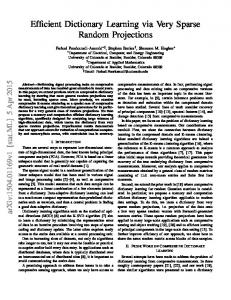
Fig. 1: Encoding of the sparse code. (a) After quantization (here δa = 1), each coefficient ak is decomposed into three variables, zk = 1(ak ), sk = sgn(ak ) and vk = max{|ak | − δa , 0}. These are respectively modeled by random variables Z ∼ Ber(ρa ), S ∼ Ber(1/2), V ∼ Exp(θa ) (only the shaded numbers are actually encoded) (b) Scheme of the mapping from continuous coefficients (random variable A), into Z , S and V . (c) Ideal codelength for the MOE model for V , − log qV (V ; κ, β). This is a smooth, concave function.

All such issues need to be considered with efficiency of computation in mind. The discussion will focus first on the traditional, single-signal case where each sample y is encoded separately from the rest. At the end of this section, we will also discuss the extension of this framework to a multi-signal case, which has several algorithmic and modeling advantages over the single-signal case, and which forms the basis for the dictionary learning algorithms described later. A. Encoding the sparse coefficients Probability model: Each coefficient in a is modeled as the product of three (non-independent) random variables, A = ZS(V + δa ), where Z = 1 implies A 6= 0, S = sgn(A), and V = max{|A| − δa , 0} is the absolute value of A corrected for the fact that V ≥ δa when Z = 1. 4 We model Z as a Bernoulli variable with P(Z = 1) = ρa . Conditioned on Z = 0, S = V = 0 with probability 1, so no encoding is needed.5 Conditioned on Z = 1, we assume P(S = −1) = P(S = 1) = 1/2, and V to be a (discretized) exponential, Exp(θa ). With these choices, P(SV |Z = 1) is a (discretized) Laplacian distribution, which is a standard model for transform (e.g., DCT, Wavelet) coefficients. This encoding scheme is depicted in Figure 1(a,b). The resulting model is a particular case of the “spike and slab” model used in statistics (see [30] and references therein). A similar factorization of the sparse coefficients is used in the Bayesian framework as well [4]. Unknown parameters: According to the above model, the resulting encoding scheme for the coefficients (sparse code) is a three-parts code: L(a) = L(z) + L(s|z) + L(a|s, z). The support z is described using the enumerative two-parts code [31], which first describes its size, kak0 , using log p bits, and then the particular
arrangement of the p
p ones in z using log kak bits. The total codelength for coding z is then L(z) = log p+log kak . This is a universal 0 0 encoding scheme, and as such is more efficient than those used previously in [11], [13]. Then, L(s|z) = kak0 bits are needed to encode s[z] , the actual signs of the non-zero coefficients. Finally, we need to encode the magnitudes of the kak0 non-zero coefficients, a[z] . We do so by considering it first as a sequence of exponentially-distributed continuous random variables, to which quantization is applied later. Since the parameter θa of the exponential is unknown,6 we use a universal model qV (·) for the class of continuous exponential distributions instead. We obtain 4

Note that it is necessary to encode S and V separately, instead of considering SV as one random variable, so that the sign of A can be recovered when |V | = 0. 5 We can easily extend the proposed model beyond S = V = 0 and consider a distribution for S, V when Z = 0. This will naturally appear as part of the coding cost. This extends standard sparse coding to the case where the non-sparse component of the vector are not necessarily zero. 6 This parameter is related to the sparsity level, and as discussed in Section II-C, is usually assumed known or determined via crossvalidation. Following [32], here we use tools from universal modeling, which permit to also automatically handle the non-stationarity of this parameter and its expected variability for different non-zero entries of a.

8

such universal model qV (V ) via a convex mixture, one of the standard techniques for this, Z +∞ θ qV (V ; κa , βa ) = Γ(θ; κa , βa ) e−θ|V | dθ, 2 0

(10)

where the mixing function Γ(θ; κ, β) = Γ(κ)−1 θκ−1 β κ e−βθ , is the Gamma density function of (non-informative) shape and scale parameters κ and β . With this choice, (10) has a closed form expression, and the degenerate cases θ = 0 and θ = ∞ are given zero weight. The resulting Mixture of Exponentials (MOE) density function qV (V ), is given by (see [32] for details), qV (V ; βa , κa ) = κa βaκa (V + βa )−(κa +1) , V ∈ R+ .

Note that the universality of this mixture model does not depend on the values of the parameters κa , βa , and guided by [32], we set κa = 3.0 and βa = 50. The ideal Shannon codelength for this density function distribution is given by − log qV (V ; κa , βa ) = − log κa − κa log βa + (κa + 1) log(V + βa ). This function, shown in Figure 1(c), is non-convex, however continuous and differentiable for V > 0. Quantization: On one hand, quantizing the coefficients to a finite precision δa increases the approximation/modeling error, from y − Da to y − D [a]δa . This additional error, D(a − [a]δa ), will clearly increase with δa . On the other hand, larger δa will reduce the description length of the non-zero values of the coefficients, [v]δa . In practice, for reasonable quantization steps, the error added by such quantization is negligible compared to the approximation error. For example, for describing natural images divided in patches of 8×8 pixels, our experiments indicate that there is no practical advantage in using a value smaller than δa = 16. Consequently, our current algorithms do not attempt to optimize the codelength on this parameter, and we have kept this value fixed throughout all the experiments of Section VII. B. Encoding the error Probability model: Most sparse coding frameworks, including all the mentioned MDL-based ones, assume the error e to be solely due to measurement noise, typically of the AWGN type. However, e actually contains a significant component which is due to a systematic deviation of the model from the clean data. Following this, we model the elements of e as samples of an IID random variable E which is the linear combination of two independent variables, ˆ + N . Here N ∼ N (0, σ 2 ) represents random measurement noise in y. We assume the noise variance σ 2 E=E e e known, as it can be easily and reliably estimated from the input data (for example, taking the minimum empirical ˆ ∼ Lap(0, θe ) is a variance over a sufficient number of sub-samples). The distribution of the second variable, E Laplacian of unknown parameter θe , which represents the error component due to the model itself. The resulting continuous distribution pE (E), which we call “LG,” is the convolution of the distributions of both components (see [33] for details on the derivation), Z +∞ 1 1 1 − |E−ζ| − ζ 2 p pE (E; σe , θe ) = e 2σe2 e θe dζ 2 2θe 2πσe ζ=−∞      2 1 2θσe2 E/θe E + σe2 /θe −E + σe2 /θe −E/θ e √ √ = e e e erfc +e erfc , (11) 4θe 2σe 2σe R +∞ 2 where erfc(u) = √2π u e−t dt is the complimentary Gauss error function. The ideal codelength, − log pE (E), is shown in Figure 2(a) for various parameter values. This function is convex and differentiable on R, which is nice for optimization purposes. Figure 2(b) shows its derivative, or so called “influence function” in robust statistics. It can be verified that − log pE (E) behaves like a Laplacian with parameter θe for large values of E . Further, since its derivative is bounded, the influence of outliers is diminished. In fact, − log pE (E) is easily verified to be a ψ -type M-estimator, a family of functions used in robust statistics (see [17]). Thus, using this model, we obtain an information-theoretic robust estimator, which is consistent with the motivations leading to its use in our framework, and which has a significant practical impact in the experimental results. Unknown parameters: Since θe is unknown, encoding e efficiently calls for the use of universal codes. In this case, again, we employ a mixture model. Since the parameter θe comes from the underlying Laplacian component, we again use a Gamma for the mixing function, Z +∞ 2 qE (E; σe , κe , βe ) = Γ(θ; κe , βe )pE (E; σe2 , θ)dθ. (12) 0

9

Fig. 2: Residual probability model. (a) Ideal codelength function of the “LG” distribution, − log pE (E), (b) LG influence function, that is, (− log pE (y))0 , (c) universal mixture for the LG model (MOEG), (d) MOEG influence function.

We call this model MOEG. As with the MOE model, the universality of this model is guaranteed by the theory for the choice of its underlying mixing function, for any (non-informative) κe and βe . In this case, we use κe = 3.0 and βe = δe . Also, we know from the discussion above that σe2 can be easily and reliably estimated from the data. Thus, we can say that the model for E is parameter-free in this case as well. Figure 2(c) shows the numerical evaluation of the ideal Shannon codelength − log qE (E; σe2 , κe , βe ), which is non-convex. However, it is twice differentiable everywhere, again a desirable property for optimization purposes (more on this in sections V and VI). As with the LG distribution, − log qE (E) is an ψ -type M-estimator, in this case, a redescending M-estimator, since its derivative (Figure 2(d)) vanishes to 0 at ∞. As such, − log qE (E), derived from the universal model corresponding to pE (E), can reject outliers even more aggressively than − log pE (E), again marrying robust statistics with information theory in a natural way. Quantization: To losslessly encode finite-precision input data such as digital images, the quantization step of the error coefficients needs not be more than that of the data itself, δy , and we simply quantize the error coefficients uniformly with step δe = δy . For example, for 8-bit digital images, we set δe = δy = 1. C. Model for the dictionary Probability model: Dictionary learning practice shows that learned atoms, unsurprisingly, present features that are similar to those of the original data. For example, the piecewise smoothness of small image patches is to be expected in the atoms of learned dictionaries for such data. This prior information, often neglected in dictionary learning algorithms, needs to be taken into account for encoding such atoms efficiently. We embody such information in the form of predictability. This is, we will encode an atom d ∈ Rm as a sequence of causal prediction residuals, b ∈ Rm , bi+1 = di+1 − d˜i+1 (d1 , d2 , . . . , di ), 1 ≤ i < m, a function of the previously encoded elements in d. In particular, if we restrict d˜i+1 to be a linear function, the residual vector can be written as b = Wd, where W ∈ Rm×m is lower triangular due to the causality constraint (this aspect has important efficiency consequences in the algorithms to be developed in Section VI). This is depicted in Figure 3, along with the specific prediction scheme that we adopted for the image processing examples in Section VII. In √ √ this case we consider an atom d to be an m× m image patch, and use a causal bi-linear predictor where the prediction of each pixel in the dictionary atom is given by north pixel + west pixel − northwest pixel. As a general model for linear prediction residuals, we assume b to be a sequence of IID Laplacian samples of parameter θd . In principle, θd is also unknown. However, describing D is only meaningful for dictionary learning purposes, and, in that case, D is updated iteratively, so that when computing an iterate D(t) of D, we can use D(t−1) to estimate and fix θd via ML (more on this θd later in Section VI). Thus, we consider θd to be known. Quantization: When A is fixed during a dictionary learning iteration (which consists of an alternate descent between D and A), we can view (A, Y) as n input-output training pairs, and D as the ML estimator of the linear √ coefficients describing such mapping via Y = DA + E. Based on this, we use the quantization step δd = 1/ n, which is an optimal step for encoding the ML parameter in two-part codes, as described in [8, Theorem 1]. Computation: Computing L(D) is onlyPrelevant for learning purposes. In general, since kdk k2 ≤ 1, and kdk k2 ≤ √ √ √ m kdk k1 , we have that θˆd = (pm)−1 k kdk k1 ≤ (p m)−1  δd = n, and the error of using the approxima-

10

Fig. 3: Prediction scheme used for learning natural image patches dictionaries (in this example, 3×3 patches, and m = 9). An atom dk is arranged as a 3×3 patch, and a causal bi-linear predictor (shown as a 2×2 template) with ˆ k and a zero-padding (pixels outside of the patch are assumed 0) is applied to it, producing a predicted atom d 9×9 ˆ k . The previous operation can be written as bk = Wdk , with W ∈ R residual bk = dk − d the linear mapping from atom to prediction residuals corresponding to this example.

tion (9) is not significant, L(D) =

p X k=1

L(dk ) ≈

p X

{− log p(Wdk ; θd ) − m log δd } = θd

k=1

p X k=1

kWdk k1 +

mp log n + c, 2

(13)

where p(Wdk ) is the IID Laplacian distribution over the k−th atom prediction residual vector Wdk , and c is a fixed constant. For p fixed (we will later see how to learn the dictionary size p as well), the above expression is simply an `1 penalty on the atom prediction residual coefficients. As we will see in Section VI, this allows us to use efficient convex optimization tools to update the atoms. D. Extension to sequential (collaborative) coding One natural assumption that we can often make on the set of data samples Y is that, besides all being sparsely representable in terms of the learned dictionary D, they share other statistical properties. For example, we can assume that the underlying unknown model parameters, θe , ρa , θa , θd , are the same for all columns of the sparse data decomposition (E, A). Under such assumption, if we encode each column of Y sequentially, we can learn statistical information from the ones already encoded and apply it to estimate the unknown parameters of the distributions used for encoding the following ones. The general idea is depicted in Figure 4(a). Concretely, suppose we have already encoded j − 1 samples. We can then use [e1 , e2 , . . . , e(j−1) ] to estimate θe , and [a1 , a2 , . . . , a(j−1) ] to estimate θa and ρa , and “plug-in” these parameters to encode the j -th sample. This justifies the name of this encoding method, which is known in the coding literature as sequential plug-in encoding. This encoding strategy has several advantages: 1) For common parameter estimators such as ML, this method can be shown to be universal; 2) Since all distribution parameters are fixed (pre-estimated) when encoding the j -th sample, we can use the “original,” non-universal distributions assumed for modeling ej (LG) and aj (Laplacian), which have closed forms and are usually faster to compute (together with (9)) than their universal mixture counterparts; 3) Furthermore, these original distributions are convex, so that in this case, given a fixed support, we are able to exactly minimize the codelength over the non-zero coefficient values; 4) With many samples available for parameter estimation, we can potentially afford more complex models. Residual: We estimate θe in two steps. First, since the random variable E is an independent sum of two random ˆ + N , we have that var(E) = var(E) ˆ + var(N ) = var(E) ˆ + σ 2 . Now, since E ˆ is Laplacian, we variables, E = E e q ˆ = 2θ2 . Combining both equations we have that θe = 0.5 var(E) ˆ − σ 2 . With the noise variance have that var(E) e e

ˆ = (p(j − 1))−1 E[1,...,(j−1)] 2 , σe2 assumed known, and using the standard unbiased variance estimator, var( ˆ E) F we obtain q

2 θˆe = 0.5 max{(p(j − 1))−1 E[1,...,(j−1)] F − σe2 , 0},

11

Fig. 4: Collaborative encoding scheme. (a) In this example, 3 samples have already been encoded, and we are about to encode sample 4. The formulas for estimating the various model parameters are shown for j = 4, in particular those for the error and the coefficients associated to the k -th atom (the k -th row of A). (b) Markov model for the coefficients support matrix Z. Here, a sample patch y is about to be encoded. Here the first atom was only used by the pixel to the west, so that the Markov state for modeling z1 is (n, w, nw) = (0, 1, 0), and P (z1 = 1) = ρ1(0,1,0) . As for the k -th atom, only the nw pixel has used it, so that the Markov state for zk is (0, 0, 1), that is, P (zk = 1) = ρk(0,0,1) .

where the maximization guarantees that θˆe ∈ R+ . Coefficients: In the case of a, we have in principle two unknown parameters, the probability of an element being non-zero, ρa , and the scale parameter of the Laplacian governing the non-zero values, θa (both previously handled with universal models). Here, however, we extend the model, drawing from the well known empirical fact that coefficients associated to different atoms can have very different statistics, both in frequency and variance. This is typical of DCT coefficients for example (see [34]), and has been consistently observed for learned dictionaries as well [32]. Therefore, we will consider a separate set of parameters (ρka , θak ) for each row k of A, ak . We update such parameters from the coefficients observed in the respective row for the already-computed samples, (ak1 , ak2 , . . . , ak(j−1) ), and encode each k -th coefficient in aj (more specifically, in zj , and vj ), as the j -th sample P(j−1) of the respective row. Concretely, let nk1 = j 0 =1 zkj 0 be the number of non-zero coefficients observed so far in the k -th row. For ρka , we use the Krichevsky-Trofimov (KT) estimator [35], ρˆka =

nk1 + 0.5 , j

(14)

which is a universal plug-in encoding scheme for Bernoulli sequences of unknown parameter. For encoding vkj , we apply the ML estimator for the exponential family to the non-zero coefficients observed so far in the k -th row. Recalling that vkj = max{|akj 0 | − δa , 0}, the resulting estimator is given by P(j−1) j 0 =1 max{|akj 0 | − δa , 0} k ˆ θa = . nk1 Markovian dependencies: In many applications, spatially/temporally adjacent samples are statistically dependent. For example, we may assume that an atom is more likely to occur for a sample j if it has been used by, say, the (j − 1)-th sample (see also [36]). In that case, we may consider different estimations of ρk depending on the value of zk(j−1) , ρk1 = P(zkj = 1|zk(j−1) = 1), and ρk0 = P(zkj = 1|zk(j−1) = 0). In particular, for the image processing results of Section VII, we use a Markovian model which depends on three previous samples, corresponding to the (causal) neighboring west, north, and northwest patches of the one being encoded. Thus, for each atom k we will have 8 possible parameters, ρk(n,w,nw) , (n, w, nw) ∈ {0, 1}3 , where each value of (n, w, nw) indicates a possible Markov state in which a sample may occur. This is depicted in Figure 4(b). For each state (n, w, nw), we estimate ρk(n,w,nw) using (14), with the average taken over the samples which occur in the same state (n, w, nw).

12

Algorithm 1: COdelength Minimizing Pursuit Algorithm (COMPA) 1 2 3 4 5 6 7 8 9 10 11 12 13 14

Input: Data sample y, dictionary D ˆ, e ˆ Output: a initialize t ← 0; a(0) ← 0; e ← y; L(0) ← L(y, 0); g(t) ← DT e(t) ; repeat for k ← 1, 2, . . . , p do (t) ∆k ← [gk ]δa ; ˜ Lk ← L([e − ∆k dk ]δe , a + ∆k ωk ) ; end ˜ k : k = 1, . . . , p} ; L(t+1) ← min{L a(t+1) ← a(t) + ∆kˆ ωkˆ ; g(t+1) ← g(t) − ∆kˆ dkˆ ; t←t+1 ; until L(t) ≥ L(t−1) ; ˆ ← a(γ − 1) ; a ˆ ← [y − Dˆ e a] ; STOP ;

V. MDL

// g(t) correlation of current residual with the dictionary

// step ∆k is correlation, quantized to prec. δa // ωk = k-th canonical vec. of Rp

// update coefficients vector // update correlation

BASED SPARSE CODING

For the encoding problem, D is fixed (it has already been learned), and we consider encoding a single data sample y. The model selection problem here is that of choosing the model (indexed by the sparse code a) among all the models belonging to the nested family of model classes M(γ) = {a ∈ Rp , kak0 ≤ γ} , γ = 0, . . . , p, that yields the smallest codelength for describing y. In principle, this calls for finding the best model a(γ) within each model ˆ = arg min0≤γ≤p L(y, a(γ)). However, in order to be computationally efficient, class M(γ), and then selecting a and as with most sparse coding and model selection algorithms, several simplifications and approximations are needed. Let us first consider the problem of finding a(γ), a(γ) := arg min L(y, a) = arg minp − log PE (y − Da) − log P(z) − log P(s|z) − log PV (a|s, z) a∈R a∈M(γ)   p = arg minp − log PE (y − Da) − log + kak0 − log PV (a) s.t. kak0 ≤ γ. a∈R kak0

(15)

For quantized a, this is an optimization problem over a discrete, infinite domain, with a non-convex (in the continuous domain) constraint, and a non-differentiable cost function in a. Based on the literature on sparse coding, at least two alternatives can be devised at this point. One way is to use a pursuit technique, e.g., [18]. Another option is to use a convex relaxation of the codelength function, e.g., [37]. For the sake of brevity, here we will describe an algorithm loosely based on the first alternative. Details on the convex relaxation method for MDL-based sparse coding will be published elsewhere. The pursuit-like algorithm, which we call COdelength-Minimizing Pursuit Algorithm (COMPA), is summarized in Algorithm 1. This is a non-greedy cross-breed between Matching Pursuit (MP) and Forward Stepwise Selection (FSS) [38]. As with those methods, COMPA starts with the empty solution a(0) = 0, and updates the value of one single coefficient at each iteration. Then, given the current correlation g(t) = De(t) between the dictionary hatoms i (t) and the current residual, each k -th coefficient in a(t) is tentatively incremented (or decremented) by ∆k = gk , ˆ k is computed in each case. The coefficient that produces the smallest L(y, ˆ and a candidate codelength L a) is (t+1) updated to produce a . The logic behind this procedure is that the codelength cost of adding a new coefficient to the support is usually very high, so that adding a new coefficient only makes sense if its contribution is high enough to produce some noticeable effect in the other parts of the codelength. A variant of this algorithm was also implemented where, ˆ k . However, this variant for each candidate k , the value of the increment ∆k was refined in order to minimize L turned out to be significantly slower, and the compression gains where below 0.01 bits per sample (uncompressed codelength is 8 bits per sample). Assuming that L(t) is unimodal, the algorithm stops if the codelength of a new iterate is larger than the previous one. To assess the validity of this assumption,

we also implemented a variant which stops, as MP or FSS, when the residual-coefficients correlation g(t) ∞ is no longer significant, which typically requires many more iterations. With this variant we obtained a negligible improvement of 0.004 bits per sample, while increasing the computational cost about three times due to the extra iterations required.

13

Fig. 5: Typical evolution of the COMPA algorithm. (a) coefficients. (b) codelength. The best iterate (code) is marked with a black circle. Also note that describing the support (L(Z)) actually takes more bits than describing the non-zero values (L(V )).

Algorithm 2: MDL-based dictionary learning via forward selection. 1 2 3 4 5 6 7 8 9

Input: Data Y ˆ D) ˆ Output: (A, initialize p ← 0; A(0) ← ∅; D(0) ← ∅; E(0) ← Y; L(0) ← L(E(0), A(0), D(0)) ; repeat ˜ ← u1 , UΣV| = E(p) // Initial value of new atom is the left-eigenvector associated to the largest singular value of E(t) . d ˜ ] // Initial dictionary for optimization below. D0 ← [ D(p) | d (A(p + 1), D(p + 1)) ← arg min(A,D)∈M(p+1) L(E, A, D) // Optimize dict. via Algorithm 3 p←p+1 ; L(p) ← L(E(p), A(p), D(p)) ; until L(p) ≥ L(p − 1) ; ˆ ← A(p − 1); D ˆ ← D(p − 1); A

VI. MDL

BASED DICTIONARY LEARNING

Given that our sparse coding algorithm in Section V can select the best support size γ for each sample in Y, the definition of the model class M(γ, p) given in Section III, which assumes the same γ for all samples in Y, is no longer appropriate (we could of course add 0-weight coefficients to make γ equal for all data). Instead, for dictionary learning, we consider the model class family M(p) = {(A, D), D ∈ Rm×p , aj ∈ M(γ; D), j = 1, . . . , n}, where M(γ; D) is the model class family of sparse codes based on a fixed dictionary D defined in Section V, with the dependency on D made explicit. It is easy to see that the model classes M(p) are nested. We now need to solve (A(p), D(p)) = arg

min

L(E, A, D),

(A,D)∈M(p)

(16)

ˆ D) ˆ = (A(ˆ for p = 0, 1, . . ., and then choose (A, p), D(ˆ p)) with the optimal dictionary size pˆ = arg min {L(E, A(p), D(p)) : p = 0, 1, . . .} . p

As with sparse coding, here we exploit the nested nature of the model classes to speed up the model selection. For this, we propose a forward-selection algorithm, described in Algorithm 2, which starts from M(0) (the empty dictionary), and then approximates the best model in M(p + 1) by adding a new atom to the dictionary computed for M(p) and then invoking Algorithm 3, which is discussed in depth in the next subsection. A backward-selection algorithm was also developed which first learns the model for M(pmax ) via (3), where pmax is a given maximum dictionary size, and then prunes the less frequently used atoms until no further decrease in codelength is observed. This algorithm allows us to provide especially-constructed initial dictionaries for Algorithm (3), e.g., an (overcomplete) DCT frame, which can be critical for finding good local minima of the non-convex problem (16). We do this for example to learn a dictionary for the whole class of natural images, see Section VII.

14

Algorithm 3: MDL-based dictionary learning for a given size p 1 2 3 4 5 6 7 8 9

Input: Data Y, initial dictionary D0 , multiplier λ, η ˆ D) ˆ Output: Local-optimum (A, initialize D(0) = D0 , t = 1 ; repeat for j = 1, . . . , n do (t) aj ← arg minA L(e, a, D(t−1) ) ; end  Update plug-in parameters: θe , (θak , ρka ), k = 1, . . . , p , θd ; (t) D ← arg minD L(E, A, D) ; t ← t + 1 ;

until

(t)

D −D(t−1)

kD(t) k2

2

≤;

A. Optimizing the dictionary for fixed p For fixed p, and given an initial D, Algorithm 3 adapts the atoms of D to fit the training data Y. At the high level, our algorithm is very similar to the traditional approach of alternate minimization over (A, D). However, there are a number of important differences, namely: 1) The cost function minimized is now the cumulative codelength of describing Y, L(E, A, D); 2) Minimizing over A is done sample by sample following Section V; 3) Since D needs to be described as well, it has an associated codelength (see Section IV-C), resulting in regularized dictionary update, described below; 4) in a cross-breed between Expectation-Maximization, and plug-in estimation, we estimate the model parameters for the current iterate (E(t) , A(t) , D(t) ), from the accumulated statistics of previous iterates  0 0 0 (E(t ) A(t ) , D(t ) ), t0 = 1, . . . , t − 1 . At the end of the learning process, these parameters are “saved” as part of the learned model and can be used for modeling future data along with D. At the t-th iteration of the alternate minimization between D and A, with A(t) just computed and kept fixed, the dictionary step consists of solving the sub-problem D(t) = arg min L(Y, A(t) , D) = arg min L(Y|A(t) , D) + L(D). m×p m×p D∈R

D∈R

According to Section IV-C, we have L(D) =

1 (t) d

θ

Pp

k=1 kWdk k1 ,

(t)

where θd

=

1 mp

Pp

k=1

(t−1) | i=1 |dik

Pm

is the

Laplacian MLE of θd based on D(t−1) . Correspondingly, the data fitting term, via (9) and disregarding the constant Pn Pm (t) (t) (t) 2 terms, is given by L(Y|A(t) , D) = L(Y − DA(t) |θe , σe2 ) = j=1 i=1 − log LG(yij − (DA )ij ; θe , σe ), (t)

where θe is the estimator of θe given E = Y − D(t−1) A(t) (see Section IV-D) and σe2 is assumed known. The problem can now be written as, p X (t) D(t) = arg min L(Y − DA(t) |θe(t) , σe2 ) + θd kWdk k1 . (17) D

k=1

For general W, the optimization of (17) is challenging since none of the above terms are separable, in particular, the non-differentiable `1 term. However, since W is easily invertible (as described in Section IV-C, it is lower triangular with 1’s in the diagonal), we can perform a change of variables and solve the equivalent problem in the prediction residual matrix U = WD instead, p X (t) −1 (t) (t) 2 ˆ U = arg min L(Y − W UA |θe , σe ) + θd kUk k1 . (18) U

k=1 (t)

Since the regularization term in (18) is decoupled in the elements of U, and L(Y − W−1 UA|θe , σe2 ) is convex and differentiable in U (see Figure 2(a)), (18) can be efficiently solved using the existing techniques for separable non-differentiable regularization terms. In our case, we employ the backtracking variant of FISTA [23], focusing on an efficient numerical evaluation of each step. VII. E XPERIMENTAL RESULTS A. Coding performance The first experiment in this section assesses the ability of our coding scheme to actually produce a compressed description of the data, in this case 8-bit gray-scale images. To this end, a dictionary D was learned using the

15

backward-selection algorithm, for the training samples from the Pascal’06 image database, 7 converted to 8-bit gray-scale images and decomposed into 8×8 patches. The initial dictionary was an overcomplete DCT frame with p = 256. The resulting global dictionary D has p = 250 atoms. We then encoded the testing samples from the same database, obtaining an average codelength of 4.1 bits per pixel (bpp), confirming the ability of our model to produce a compressed description of the data. B. Learning performance We compare the performance of the forward and backward dictionary learning algorithms proposed in Section VI by applying each method to learn a dictionary for the standard “Boats” image (taken from the SIPI database, 8 along with “Lena,” “Barbara” and “Peppers” used in the following experiments), and then measuring the final codelength and computation time. For the backward case, the initial dictionary is the global dictionary learned in the previous experiment. As for the forward method, we also include a faster “partial update” variant which performs a few (10) iterations of Algorithm 3 after adding a new atom, instead of allowing it to converge. The backward method produced a dictionary of size p = 170, yielding a compression level of 5.13bpp at a computational cost of 3900s. For the convergent forward method, a dictionary with p = 34, yielding 5.19bpp and requiring 800s. Finally, the forward method resulted in a dictionary of size p = 20, 5.22bpp, and required 150s. In all cases, the running times were measured for a parallelized C++ implementation running on an Athlon Phenom II X6 at 2.6GHz). In summary, all three methods reach similar, significant, compression levels. Slightly better results are obtained with the backward method, at the cost of a significant increase in computational time. On the other hand, the partial forward variant is significantly faster than the other two, yielding similar codelengths. C. Denoising of natural images The task in this case is to estimate a clean image from an observed noisy version whose pixels are corrupted by AWGN of known variance σe2 . Here Y contains all (overlapping) 8×8 patches from the noisy image. The denoising algorithm proceeds in two stages. In the first one, a dictionary D is learned from the noisy image patches Y. We use the backward selection algorithm since it allows us to use the global dictionary as the starting point, a common practice in this type of problems, [25], [27]. Secondly, the clean patches are estimated as sparse combinations of atoms from D. In our case, the second stage admits two variants. The first one is a rate-distortion (RD) procedure ˆ j is estimated using a distortionakin to the traditional method used for example in [25], where each clean sample y constrained formulation. In our case, we minimize the codelength (or “rate”) of describing yj up to a prescribed 2 . Here we ˆ j = Dˆ ˆj = arg minu L(u) s.t. kyj − Duk2 ≤ CσN distortion proportional to the noise level, y aj , a use C = 1.0. The second variant, coined “post-thresholding” (PT) is more consistent with the learning phase, and is truly parameter-free, since the estimation derives from the same codelength minimization procedure used for ˜ j = D˜ ˜j = arg minu L(u) + L(yj |u). learning the dictionary D. In this case we obtain an initial estimate y aj , a ˜ = yj − y ˜ j may contain a However, according to the model developed in Section IV-B, the encoding residual e ˜ as clean data corrupted by noise of significant portion of clean data due to modeling errors. We can then think of e variance σe2 . To extract the clean portion, we solve another codelength-minimization sub-problem, this time with a ¯j = arg minu σ12 k˜ Gaussian prior for the error, and a Laplacian prior for the clean part, e ej − uk2 + ˆ1 kuk1 , where θe e p ˆj = y ˜j + e ¯j . In θˆe = 0.5 max{0, var(˜ ej ) − σe2 }, following Section IV-D. We then compute the final estimate as y either variant, the model used for L(a) includes the Markovian dependency between the occurrence of each atom in a patch and its previously-encoded neighbors, as described in Section IV-D. Denoising performance is summarized in Figure 6, along with a detail of the result for σe = 10 for the “Boats” image in Figure 6. In all cases, there is a 1 to 5 dB improvement over the best MDL-based results in [15], thus showing the relevance of overcoming the limitations in previous MDL applications to sparse coding. Both the RD and PT methods yield results which are comparable to those of [25], which depend significantly on several carefully tuned parameters.9 While the RD variant performs better than PT in terms of PSNR, PT is faster and 7 8 9

http://pascallin.ecs.soton.ac.uk/challenges/VOC/databases.html http://sipi.usc.edu/database/database.php?volume=misc&image=38#top

To the best of our knowledge, these results, as well as those in [25], are among the best that can be obtained for gray-scale images without using multi-scale and/or spatial aggregation of patches as in [39], [40].

16

σe = 10 lena barbara boat peppers σe = 20 lena barbara boat peppers

PT 34.9 33.0 33.1 34.1 PT 32.0 29.7 29.5 31.7

RD 35.2 33.8 33.2 34.4 RD 32.2 30.6 30.3 31.6

[15] 32.4 29.4 30.5 32.2 [15] 29.4 25.7 27.5 29.4

[25] 35.5 34.4 33.6 34.3 [25] 32.4 30.8 30.3 30.8

Fig. 6: Denoising results. Left table: denoising performance, in PSNR, of K-SVD [25], MDL denoising [15], and the Post-Thresholding (PT) and Rate-Distortion (RD) denoising variants. Images, top row: clean “Boats”, noisy version, learned dictionary for this image (final p = 248), image recovered using RD. Images, bottom row: image ˜ j obtained in the PT method, its residual, portion of residual that was reconstructed from the initial estimation y added back, final PT estimation.

tends to produce less artifacts than RD, thus resulting in more visually pleasant images than RD. This, which can be clearly seen in Figure 6, occurs in all other cases as well. Including the Markov dependency in L(a) produced an average improvement of up to 0.2dB. D. Texture mosaic segmentation Here we are given c images with sample textures, and a target mosaic of textures,10 and the task is to assign each pixel in the mosaic to one of the textures. Again, all images are decomposed into overlapping patches. This time a different dictionary is learned for each texture using patches from corresponding training images. In order to capture the texture patterns, a patch width w = 16 was used. Then, each patch in the mosaic is encoded using all available dictionaries, and its center pixel is assigned to the class which produced the shortest description length for that patch. This seemingly natural procedure results in a success rate of 77%, which is consistent with the second picture of Figure 7. The problem is that this procedure is inconsistent with the learning formulation, because each dictionary is adapted to minimize the average codelength of describing each patch in the respective texture. Therefore, good results can only be expected if the decision is made for groups of patches simultaneously, that is, by considering the cumulative codelength of a set of patches. We implement this by deciding on each patch on the basis of comparing the average codelength obtained with each dictionary for encoding that patch and all patches in a circular neighborhood with a radius of 20 pixels. The success rate in this case is 95.3%, which is comparable to the state-of-the art for this type of problems (see for example [41], which learns sparse models for explicitly maximizing the success rate). The Markovian model improved our results by 1%. E. Low-rank matrix approximation The low-rank matrix approximation family of problems (see [42] for a review) can be seen as an extension to the problem of sparse coding where sparsity is substituted by matrix rank. Concretely, the task is to recover a matrix A ∈ Rm×n from an incomplete and/or corrupted observation Y, under the assumption that the rank of A, rank(A), is small. As with sparse coding, rank(A) is relaxed using the `1 equivalent for matrix rank, which is P the nuclear norm, kAk∗ := i σi (A), where σi (A) is the i-th singular value of A. It has been shown in [42] 10

Taken from http://www.ux.uis.no/∼tranden/.

17

Fig. 7: Left to right: Texture mosaic, dictionaries learned for each class (note the automatically learned different sizes), patch-wise codelength-based classification map –each shade of gray corresponds to a texture class – (77.0% success rate), classification map obtained by averaging the codelength over a neighborhood of patches (95.4% success rate).

that, under certain assumptions on rank(A), the following estimation function is able to recover A from a noisy observation Y, and with a significant fraction of its coefficients arbitrarily corrupted, p ˆ = arg min kWk + λ kY − Wk , λ = 1/ max{m, n}. A (19) ∗ 1 W

A common proof of concept is to use this framework for robust background estimation in camera surveillance video sequences [43], and we apply our proposed framework for the same application. To perform our MDL-based model selection within this formulation, we solve (19) for increasing values of λ, obtaining a low-rank approximation to A, (A(λ), E(λ) = Y − A(λ)), which we encode using the universal models described in Section IV. We modified the algorithm described in [44] to allow for warm restarts, using the solution for the previous λ as a starting point for the next λ for faster convergence. Consistently with the `1 fitting term of (19), we encode the non-zero values of E(λ) as a Laplacian sequence of unknown parameter. To exploit the potential sparsity in E(λ), the locations of the non-zero values are encoded, as in IV-A, using an enumerative two-parts code for Bernoulli sequences of unknown parameter. To exploit low-rank in the encoding, the matrix A(λ) is encoded via its reduced SVD decomposition A(λ) = U(λ)Σ(λ)V(λ)| . For rank(A(λ)) = r, we have that U(λ) ∈ Rm×r are the left-eigenvectors, Σ ∈ Rr×r is the diagonal matrix whose diagonal are the non-zero singular values of A(λ), and V(λ) ∈ Rr×n are the right-eigenvectors of A(λ). Each column of U is encoded (in this video example) as a smooth image via a causal bilinear predictor identical to the one used for predictive coding of D in IV-C, using a Laplacian model for the prediction residuals. Each column of V is encoded as a smooth one-dimensional sequence, using a zero order predictor (the predicted value for the next coefficient is the previous coefficient value), with a Laplacian prior on the prediction residuals. Finally, the values of Σ, which can be arbitrary, are quantized and encoded using the universal code for integers [45]. The encoding method is very simple, with all unknown parameters encoded using a two-parts code, and codelenghts for the discretized Laplacian pre-computed in look-up tables. Quantization for this case is as follows: the codelength associated with the r non-zero singular values is negligible, and we minimize unwanted distortion encoding them with high precision (1e − 16). As forpthe columns pof U and V, they all have unit norm, so that the average magnitude of their √ elements are close to 1/m and 1/n respectively. Based on this, our algorithm √ encodes the data with δu = Q/ m as the precision for encoding U, and δv = Q/ m for V, for several values of Q in (0, 1), keeping the one producing the smallest codelength. The MDL-based estimation algorithm then chooses the model for which the codelength L(Y; λ) = L(U(λ)) + L(Σ(λ)) + L(V(λ)) is minimized. As in [43], here we show results for two sequences taken from [46]: “Lobby” (Figure 8(a)), and “ShoppingMall” (Figure 8(b)). Full videos can be viewed at http://www.tc.umn.edu/∼nacho/lowrank/. In both cases, the recovered backgrounds are very accurate. In particular, for the Lobby sequence, the selected model captures just the eigenvectors needed to recover the background along with its lighting changes, including corrections for local shadows, leaving out only the people passing by. VIII. C ONCLUDING REMARKS We have presented an MDL-based sparse modeling framework, which automatically adapts to the inherent complexity of the data at hand using codelength as a metric.

18

(a) Results for “Lobby” sequence, featuring a room with lights that are switched off and on. The rank of the approximation for this case is rank = 10. The moment where the lights are turned off is clearly seen here as the “square pulse” in the middle of the first two right-eigenvectors (bottom-right). Also note how u2 (top-right) compensates for changes in shadows.

(b) Results for “ShoppingMall”, a fixed camera looking at a crowded hall. In this case, the rank of the approximation decomposition is rank = 7. Here, the first left-eigenvector models the background, whereas the rest tend to capture people that stood still for a while. Here we see the “phantom” of two such persons in the second lefteigenvector (top-right).

Fig. 8: Low-rank approximation results. Both figures show the first two left-eigenvectors as 2D images at the top, two sample frames from the approximation error sequences in the middle, which should contain the people that were removed from the videos, and the curve L(λ) and the right-eigenvalues, scaled by Σ (representing the “activity” of each left-eigenvector along time), at the bottom.

The framework features a sparse coding algorithm and automatic tuning of the sparsity level on a per-sample basis, including a sequential collaborative variant which adapts the model parameters as it processes new samples, and two dictionary learning variants which learn the size of the dictionaries from the data. In all cases, the informationtheoretic formulation led to robust coding and learning formulations, including novel robust metrics for the fitting term (LG and MOEG), and robust `1 -based dictionary regularization term. This formulation also allowed us to easily incorporate more prior information into the coding/learning process, such as Markovian spatial dependencies, by means of simple modifications to the probability models used. As a result, the framework can be applied out-of-the-box to very different applications, from image denoising to low-rank matrix approximation, obtaining competitive results in all the cases presented, with minimal interaction from the user. R EFERENCES [1] A. Bruckstein, D. Donoho, and M. Elad, “From sparse solutions of systems of equations to sparse modeling of signals and images,” SIAM Review, vol. 51, no. 1, pp. 34–81, Feb. 2009. [2] R. Rubinstein, A. Bruckstein, and M. Elad, “Dictionaries for sparse representation modeling,” Proceedings of the IEEE, vol. 98, no. 6, pp. 1045–1057, June 2010. [3] J. Wright, Y. Ma, J. Mairal, G. Sapiro, T. Huang, and S. Yan, “Sparse representation for computer vision and pattern recognition,” Proceedings of the IEEE, vol. 98, no. 6, pp. 1031–1044, June 2010.

19

[4] M. Zhou, H. Chen, J. Paisley, L. Ren, L. Li, Z. Xing, D. Dunson, G. Sapiro, and L. Carin, “Nonparametric Bayesian dictionary learning for analysis of noisy and incomplete images,” submitted to IEEE Trans. Image Processing, 2011. [5] H. Akaike, “A new look at the statistical model identification,” IEEE Transactions on Automatic Control, vol. 19, pp. 716–723, 1974. [6] G. Schwartz, “Estimating the dimension of a model,” Annals of Statistics, vol. 6, no. 2, pp. 461–464, 1978. [7] J. Rissanen, “Modeling by shortest data description,” Automatica, vol. 14, pp. 465–471, 1978. [8] J. Rissanen, “Universal coding, information, prediction, and estimation,” IEEE Trans. IT, vol. 30, no. 4, pp. 629–636, 1984. [9] A. Barron, J. Rissanen, and B. Yu, “The minimum description length principle in coding and modeling,” IEEE Trans. IT, vol. 44, no. 6, pp. 2743–2760, 1998. [10] T. Cover and J. Thomas, Elements of Information Theory, John Wiley and Sons, Inc., 2 edition, 2006. [11] N. Saito, “Simultaneous noise suppression and signal compression using a library of orthonormal bases and the MDL criterion,” in Wavelets in Geophysics, E. Foufoula-Georgiou and P. Kumar, Eds., pp. 299–324. New York: Academic, 1994. [12] H. Krim and J.-C. Pesquet, “On the statistics of best bases criteria,” Tech. Rep., MIT LIDS, 1995. [13] P. Moulin and J. Liu, “Analysis of multiresolution image denoising schemes using generalized-Gaussian and complexity priors,” IEEE Trans. IT, April 1999. [14] J.Rissanen, “MDL denoising,” IEEE Trans. IT, vol. 46, no. 7, pp. 2537–2543, 2000. [15] T. Roos, P. Myllym¨aki, and J. Rissanen, “MDL denoising revisited,” IEEE Trans. SP, vol. 57, no. 9, pp. 3347–3360, 2009. [16] I. Ram´ırez and G. Sapiro, “Sparse coding and dictionary learning based on the MDL principle,” in Proc. of ICASSP 2011, Prague, Czech. Republic, May 2011. [17] P. J. Huber, “Robust estimation of a location parameter,” Annals of Statistics, vol. 53, pp. 73–101, 1964. [18] S. Mallat and Z. Zhang, “Matching pursuit in a time-frequency dictionary,” IEEE Trans. SP, vol. 41, no. 12, pp. 3397–3415, 1993. [19] R. Tibshirani, “Regression shrinkage and selection via the LASSO,” Journal of the Royal Statistical Society: Series B, vol. 58, no. 1, pp. 267–288, 1996. [20] E. J. Cand`es, “Compressive sampling,” Proc. of the International Congress of Mathematicians, vol. 3, Aug. 2006. [21] D. L. Donoho and I.M Johnston, “Ideal spatial adaptation by wavelet shrinkage,” Biometrika, vol. 81, no. 3, pp. 425–455, September 1994. [22] J. Friedman, H. Hastie, and R. Tibshirani, “Regularized paths for generalized linear models via coordinate descent,” Journal of Stat. Soft., vol. 33, no. 1, 2008. [23] A. Beck and M. Teboulle, “A fast iterative shrinkage-thresholding algorithm for linear inverse problems,” SIAM Journal on Imaging Sciences, vol. 2, no. 1, pp. 183–202, 2009. [24] B. Efron, T. Hastie, I. Johnstone, and R. Tibshirani, “Least angle regression,” Annals of Statistics, vol. 32, no. 2, pp. 407–499, 2004. [25] M. Aharon, M. Elad, and A. Bruckstein, “The K-SVD: An algorithm for designing of overcomplete dictionaries for sparse representations,” IEEE Trans. SP, vol. 54, no. 11, pp. 4311–4322, Nov. 2006. [26] J. Mairal, F. Bach, J. Ponce, and G. Sapiro, “Online learning for matrix factorization and sparse coding,” Journal of Machine Learning Research, vol. 11, pp. 19–60, 2010. [27] J. Mairal, M. Elad, and G. Sapiro, “Sparse representation for color image restoration,” IEEE Trans. IP, vol. 17, no. 1, pp. 53–69, Jan. 2008. [28] P. Gr¨unwald, The Minimum Description Length Principle, MIT Press, June 2007. [29] Y. Shtarkov, “Universal sequential coding of single messages,” Probl. Inform. Transm., vol. 23, no. 3, pp. 3–17, July 1987. [30] H. Ishwaran and J. S. Rao, “Spike and slab variable selection: Frequentist and Bayesian strategies,” Annals of Statistics, vol. 33, no. 2, pp. 730–773, 2005. [31] T. M. Cover, “Enumerative source encoding,” IEEE Trans. IT, vol. 19, no. 1, pp. 73–77, 1973. [32] I. Ram´ırez and G. Sapiro, “Universal regularizers for robust sparse coding and modeling,” Submitted. Preprint available in arXiv:1003.2941v2 [cs.IT], August 2010. [33] G. Motta, E. Ordentlich, I. Ramirez, G. Seroussi, and M. Weinberger, “The iDUDE framework for grayscale image denoising,” IEEE Trans. IP, vol. 20, no. 1, pp. 1–21, Jan. 2011. [34] E. Lam and J. Goodman, “A mathematical analysis of the DCT coefficient distributions for images,” IEEE Trans. IP, vol. 9, no. 10, pp. 1661–1666, 2000. [35] R. E. Krichevsky and V. K. Trofimov, “The performance of universal encoding,” IEEE Trans. IT, , no. 2, pp. 199–207, 1981. [36] M. Zhou, H. Yang, G. Sapiro, D. Dunson, and L. Carin, “Dependent hierarchical beta process for image interpolation and denoising,” in AISTATS, 2011. [37] S. Chen, D. Donoho, and M. Saunders, “Atomic decomposition by basis pursuit,” SIAM Journal on Scientific Computing, vol. 20, no. 1, pp. 33–61, 1998. [38] T. Hastie, R. Tibshirani, and J. Friedman, The Elements of Statistical Learning: Data Mining, Inference and Prediction, Springer, 2nd edition, Feb. 2009. [39] K. Dabov, A. Foi, V. Katkovnik, and K. Egiazarian, “Image denoising by sparse 3d transform-domain collaborative filtering,” IEEE Trans. IP, vol. 16, no. 8, pp. 2080–2095, August 2007. [40] J. Mairal, F. Bach, J. Ponce, G. Sapiro, and A. Zisserman, “Non-local sparse models for image restoration,” in ICCV, Oct. 2009, pp. 2272–2279. [41] J. Mairal, F. Bach, J. Ponce, G. Sapiro, and A. Zisserman, “Discriminative learned dictionaries for local image analysis,” in Proc. IEEE CVPR, Anchorage, USA, June 2008. [42] E. Cand`es, X. Li, Y. Ma, and J. Wright, “Robust principal component analysis?,” Journal of the ACM, vol. 58, no. 3, May 2011. [43] J. Wright, A. Ganesh, S. Rao, Y. Peng, and Y. Ma, “Robust principal component analysis: Exact recovery of corrupted low-rank matrices by convex optimization,” in Adv. NIPS, Dec. 2009. [44] Z. Lin, M. Chen, and Y. Ma, “The Augmented Lagrange Multiplier Method for exact recovery of corrupted low-rank matrices,” http://arxiv.org/abs/1009.5055.

20

[45] J. Rissanen, “A universal prior for integers and estimation by minimum description length,” Annals of Statistics, vol. 11, no. 2, pp. 416–431, 1983. [46] L. Li, W. Huang, I. Gu, and Q. Tian, “Statistical modeling of complex backgrounds for foreground object detection,” IEEE Trans. IP, vol. 13, no. 11, pp. 1459–1472, 2004.