Noname manuscript No. (will be inserted by the editor)
An MIP-based Interval Heuristic for the Capacitated Multi-level Lot-sizing Problem with Setup Times Tao Wu · Leyuan Shi · Jie Song
The paper has been published in Annals of Operations Research
Abstract This paper considers the capacitated multi-level lot-sizing problem with setup times, a class of difficult problems often faced in practical production planning settings. In the literature, relax-and-fix is a technique commonly applied to solve this problem due to the fact that setup decisions in later periods of the planning horizon are sensitive to setup decisions in the early periods but not vice versa. However, the weakness of this method is that setup decisions are optimized only on a small subset of periods in each iteration, and setup decisions fixed in early iterations might adversely affect setup decisions in later periods. In order to avoid these weaknesses, this paper proposes an extended relax-and-fix based heuristic that systematically uses domain knowledge derived from several strategies of relax-and-fix and a linear programming relaxation technique. Computational results show that the proposed heuristic is superior to other well-known approaches on solution qualities, in particular on hard test instances. Keywords Capacitated Multi-level Lot-sizing · Relax-and-fix · MIP-based Interval Heuristic · Linear Programming.
1 Introduction This paper studies the Capacitated Lot-sizing Problem with Setup Times and Multiple Levels (CLST-ML), a very challenging problem faced in production systems. The problem aims to schedule production over a pre-defined, finite time horizon while minimizing total cost and meeting all customer demands, where Tao Wu, corresponding author Department of Industrial and Systems Engineering, University of Wisconsin-Madison, Madison, WI 53706, USA Work carried out at University of Wisconsin-Madison E-mail:
[email protected] Leyuan Shi Department of Industrial and Systems Engineering, University of Wisconsin-Madison, Madison, WI 53706, USA Department of Industrial Engineering and Management, Peking University, Beijing 100871, China
Jie Song Department of Industrial and Systems Engineering, University of Wisconsin-Madison, Madison, WI 53706, USA Department of Industrial Engineering and Management, Peking University, Beijing 100871, China
2
Tao Wu et al.
complex bill-of-materials structures might complicate the problem further. The setup costs and inventory holding costs are usual components of the objective function, and the output of the model is a plan detailing setups as well as production and inventory quantities in each period and for each level. Effective solution of this problem is crucial for the cost performance of any production and inventory control system, where material requirements planning systems are used in manufacturing practice, though with serious limitations such as lacking proper handling of system capacities. As lot-sizing problems are complex and practical problems to be solved on a regular basis, researchers and practitioners have been interested in finding efficient solution approaches for decades. Of the classes of lot-sizing problems, the multi-item and/or multi-level lot-sizing problems have been intensively researched, as these problems represent the practical most realistically. Furthermore, these problems are computationally challenging. Of the previous research, Kuik and Salomon (1990) developed a simulated annealing heuristic for solving the multi-level lot-sizing problem, whereas Millar and Yang (1994) proposed two Lagrangian relaxation-based algorithms for solving the capacitated multi-item lot-sizing problem. Ozdamar and Bozyel (2000) proposed a heuristic that combines generic algorithms and simulated annealing to solve the capacitated multi-item lot-sizing problem. Hung et al. (2003) proposed a tabu search heuristic for lotsizing problems involving multiple products, multiple resources, multiple periods, setup times, and setup costs. Tempelmeier and Buschkuhl (2009) proposed a Lagrangian relaxation based heuristic for the dynamic capacitated multi-level lot-sizing problem with linked lot sizes and with general product structures. Almada-Lobo and James (2010) proposed a heuristic that incorporates a tabu search and a neighborhood search meta-heuristic to solve the capacitated multi-item lot-sizing and scheduling problem. Wu and Shi (2011) theoretically showed relationships of various Mixed Integer Programming (MIP) formulations for the capacitated multi-level lot-sizing problem with setup carryover. Wu et al. (2011) proposed two MIP formulations and an optimization framework for solving the capacitated multi-level lot-sizing problem with backlogging. Of heuristics proposed for solving lot-sizing problems, the time-oriented decomposition heuristics, including relax-and-fix, are one of the most efficient heuristics that can achieve good solutions for lot-sizing problems. Belvaux and Wolsey (2000) proposed the first systematic production planning tool with the relaxand-fix technique embedded, a specialized branch and cut system for lot-sizing problems. Stadtler (2003) proposed another variant of relax-and-fix, called internally rolling schedules with time windows. Akartunalı and Miller (2009) proposed a heuristic that employs the relax-and-fix algorithm. Unlike the relax-and-fix algorithm proposed by Stadtler (2003), this heuristic always considers the entire period horizon, not only the periods in the time window. Other similar heuristics, which use the relax-and-fix algorithm in their frameworks, include Suerie and Stadtler (2003), Merc´e and Fontan (2003), Absi and Kedad-Sidhoum (2007), Sahling et al. (2009), and Wu et al. (2010). Relax-and-fix is efficient at solving this class of problems, since setup decisions in early periods of the planning horizon are insensitive to setup decisions in later periods. However, this also presents a weakness that setup decisions are optimized only on a small subset of periods in each iteration. The binary setup decision variables fixed in early iterations might adversely affect setup decisions in later periods. This is especially true for lot-sizing problems with tight capacities and high seasonality. To avoid this weakness and to enhance the strength of the method, this paper develops an MIP-based Interval Heuristic (called as MIH in the rest of the paper).
An MIP-based Interval Heuristic for the Capacitated Multi-level Lot-sizing Problem with Setup Times
3
MIH iteratively fixes setup decision variables in an efficient way by combining domain knowledge derived from solutions obtained through relax-and-fix strategies and from solutions obtained using Linear Programming (LP) relaxations. The key point of the heuristic is to systematically fix binary setup decision variables, for which different relax-and-fix strategies and an LP rounding procedures produce equivalent results. The intuition behind this idea is two folds: The first is that the value of a decision variable is much more likely to match its optimal value, when different strategies produce the same value. We make this claim empirically, based on an intensive number of computational tests on a number of small lot-sizing problems, for which the optimal solutions are known. The second intuition is that the subproblems, in which a subset of binary variables are already prefixed, are much easier to solve to optimality. Iteratively solving these small subproblems can improve feasible solutions with high probability. To show the efficiency of the proposed method, comparisons between the MIH and another state-of-the-art heuristic and a commercial MIP solver, CPLEX 11.2, have been made. The computational results show that the MIH outperforms these methods under the same computational resources. In particular, the improvement is more significant on hard problems that have tight capacities and high seasonality. The remainder of this paper is organized in four sections. Section 2 discusses several MIP formulations, and describes their advantages and disadvantages. Section 3 describes the development of the MIH. Section 4 makes comparisons of computational results between the MIH and other approaches using a number of published data sets. Finally, Section 5 makes conclusions, and gives future research directions.
2 Mixed Integer Programming Formulations
The CLST-ML problem we consider aims to produce a production plan for a number of different items over a finite horizon, as it is the practice in the manufacturing industry. This production plan details production and inventory quantities, as well as usage of overtime, and setups in all periods. The problem has an objective of minimizing total costs, which consists of setup costs, inventory holding costs, and overtime costs. For each period, demand must be satisfied, and existing capacities can be only exceeded if expensive overtime is used. Each item is processed on a single machine. We also make the following assumptions: Setup times and costs are non-sequence dependent, for the sake of simplicity. The possibility of setup carryover between periods is neglected. Also, w.l.o.g., backlogging and initial inventories are not permitted in the model. All other production costs are assumed to be fixed and independent of time, consequently no production costs are attributed in the model. Setup costs and holding costs are also assumed to be independent of time. To present the problem formulations clearly, we first present the notation.
4
Tao Wu et al.
Indices and index sets: T
number of periods.
M
number of machines.
I
number of items.
S
subset of the full period set [1,T ].
endp set of end items that have external gross demands (external demands needed by customers). l, t, p periods, l, t, p ∈ [1,T ]. m
machines, m ∈ [1, M ].
i, j
items, i, j ∈ [1, I].
ηi
set of immediate successors of item i.
Parameters: sci
setup costs for a lot of item i.
ocmt overtime costs for one unit time of machine m in period t. hci
inventory holding costs for one unit of item i in a period.
eci
echelon inventory holding costs for one unit of item i in a period.
stim setup times for item i on machine m. aim
production time required to produce one unit of item i on machine m.
gdit
gross demand for item i in period t.
gdit,s total gross demand for item i from period t to s. edit
echelon demand (marginal demands derived from the bill-of-materials structure) for item i in period t.
edit,s total echelon demand for item i from period t to s. rij
number of units of item i needed to produce one unit of the immediate successor item j.
Cmt
available capacity of machine m in period t.
BMit maximum number of item i that can be produced in t. Variables: xit
number of item i produced in period t.
sit
inventory of item i at the end of period t.
eit
echelon inventory of item i at the end of period t.
yit
binary setup decision variables.
otmt amount of overtime used on machine m in period t.
2.1 The Inventory and Lot-sizing Formulation For the CLST-ML several prominent formulations have been proposed in the literature. We first introduce the formulation proposed by Billington et al. (1983), referred to as the Inventory and Lot-sizing (I&L) model formulation due to the variables used. I&L: min
I X T X i=1 t=1
sci · yit +
I X T X i=1 t=1
hci · sit +
M X T X m=1 t=1
ocmt · otmt
(1)
An MIP-based Interval Heuristic for the Capacitated Multi-level Lot-sizing Problem with Setup Times
5
Subject to: ∀ i ∈ endp, t ∈ [1, T ]. (2)
xit + si(t−1) = gdit + sit X xit + si(t−1) = gdit + rij · xjt + sit
∀ i ∈ [1, I] \ endp, t ∈ [1, T ]. (3)
j∈ηi I X
aim · xit +
i=1
I X
stim · yit ≤ Cmt + otmt
∀ m ∈ [1, M ], t ∈ [1, T ]. (4)
i=1
xit ≤ BMit · yit
∀ i ∈ [1, I], t ∈ [1, T ]. (5)
xit ≥ 0, sit ≥ 0, si0 = 0, otmt ≥ 0, yit ∈ {0, 1}
Here, BMit is defined formally as BMit =
P
j∈ηi
∀ i ∈ [1, I], t ∈ [1, T ], m ∈ [1, M ]. (6)
rij · gdjt,T for i ∈ [1, I]\endp, t ∈ [1, T ] and BMit =
gdit,T for i ∈ endp, t ∈ [1, T ]. The objective function minimizes total setup, holding and possible overtime costs during the planning horizon. Constraints (2) and (3) ensure demand satisfaction in all periods for end- and non-end items, respectively. Constraints (4) enforce capacity requirements. Constraint set (5) ensures that no production occurs for item i in period t unless the corresponding binary setup variable, yit , takes a value of 1, in which case the amount of production is limited only by the value of BMit . The model size corresponding to the I&L formulation is relatively modest, implying that its LP relaxation is readily solvable for problem instances with a few hundred items over a large planning interval. However, the time required for proving the optimality of a given solution is often prohibitive, because the LP relaxation provides poor lower bounds and it is not adequate in general to guide the search for good feasible solutions in the branch-and-bound phase of a standard MIP solver.
2.2 The Echelon Inventory and Lot-sizing Formulation
The above I&L formulation can be represented as an alterative formulation by introducing new parameters and variables, including echelon demand parameters edit , echelon inventory holding cost parameter eci , and echelon stock variables eit . The relationships among these new parameters and variables with those in P P the I&L formulation can be defined as follows: edit = gdit + j∈ηi rij · edjt , eci = hci − j:i∈ηj rji · hcj P and eit = sit + j∈ηi rij · ejt for t ∈ [1, T ] and i ∈ [1, I]\endp, respectively, or edit = gdit , eci = hci and eit = sit for t ∈ [1, T ] and i ∈ endp, respectively. This new formulation is referred to as the Echelon Inventory and Lot-sizing (E-I&L) model formulation. E-I&L:
min
I X T X i=1 t=1
sci · yit +
I X T X i=1 t=1
eci · eit +
M X T X m=1 t=1
ocmt · otmt
(7)
6
Tao Wu et al.
Subject to: xit + ei(t−1) = edit + eit X eit ≥ rij · ejt
∀ i ∈ [1, I], t ∈ [1, T ].
(8)
∀ i ∈ [1, I]\endp, t ∈ [1, T ].
(9)
j∈ηi I X
aim · xit +
i=1
I X
stim · yit ≤ Cmt + otmt
∀ m ∈ [1, M ], t ∈ [1, T ]. (10)
i=1
xit ≤ BMit · yit xit ≥ 0, eit ≥ 0, ei0 = 0, otmt ≥ 0 yit ∈ {0, 1}
∀ i ∈ [1, I], t ∈ [1, T ]. (11) ∀ i ∈ [1, I], t ∈ [1, T ], m ∈ [1, M ]. (12) ∀ i ∈ [1, I], t ∈ [1, T ]. (13)
The echelon I&L model formulation is equivalent to the I&L model formulation. Therefore the lower bound provided by the echelon I&L model is also weak when we solve its LP relaxation problem. In order to strengthen the model formulation, strong inequalities are to be added into the model. Among those inequalities proposed by previous research, the (l, S) inequalities proposed by Barany et al. (1984) are very efficient at improving the lower bound. Moreover, there is a polynomial separation algorithm proposed by Barany et al. (1984) to generate these inequalities. The model of E-I&L after adding inequalities constraints (14) is referred to as the SE-I&L model formulation.
X t∈S
xit ≤
X
edit,l · yit + eil .
∀ i ∈ [1, I], l ∈ [1, T ], S ⊆ [1, l]. (14)
t∈S
Besides the two above formulations, the Facility Location formulation (referred as FL), originally proposed for the single item lot-sizing problem by Krarup and Bilde (1977), also has been extended to model the CLST-ML. This formulation introduces a new set of variables uitp (t ≤ p), which indicates the amount of item i produced in period t, but used to satisfy demand in period p. A drawback related with the FL formulation is that the number of real variables uitp as well as the setup constraints grow quadratically with the number of periods in the planning horizon, implying difficulty in solving large real-world CLST-ML.
3 The MIP-based Interval Heuristic This section describes the MIP-based Interval Heuristic (MIH) in detail. Before that the relax-and-fix technique and an LP rounding procedure first are described because these two techniques are incorporated in the MIH.
3.1 Relax-and-fix The relax-and-fix approach implemented here is similar to the internally rolling schedule heuristic proposed by Stadtler (2003), but much simpler. In this approach, the entire horizon of periods is divided into three parts. The first is a time window that contains several continuous periods, the second includes the periods preceding to the time window, and the third includes the periods following the time window. In the beginning stage of such an algorithmic approach, only the binary setup decision variables in the first time window (here, α is defined as the size of the time window) are restricted as being binary, while the binary variables
An MIP-based Interval Heuristic for the Capacitated Multi-level Lot-sizing Problem with Setup Times
7
in the remaining periods are relaxed so as to be continuous variables. According to the resulting solution using an MIP solver, only the binary variables in the first few periods within the time window (here, the size of such periods is defined as β (β ≤ α)) are fixed. The next α periods (from period α +1 to α + β) then are processed in the same manner until all binary variables are fixed. In the example shown in Figure 1, α is equal to 4, and β is equal to 2.
Periods = 1 1st iteration
2
3 4
5
6
7
8
………
T
Descriptions:
………
2nd iteration
………
3rd iteration
………
Interval of time with binary setup variables Interval of time with fixed setup variables Interval of time with relaxed setup variables
Fig. 1: Relax-and-fix
3.2 The LP Rounding Procedure The LP rounding procedure is to obtain a binary solution rounded from several LP relaxation solutions for setup decision variables. Note that this binary solution is not necessarily feasible for the original problem. The purpose of obtaining this binary solution is to compare it with other binary solutions obtained from relax-and-fix, check whether or not they are equivalent, and help make decisions of which setup decision variables to be fixed. The intuition of this procedure is that this new binary solution can provide good matches on optimal solutions according to our computational experience on small-size lot-sizing problems. To see how to get this binary solution, suppose relax-and-fix is implemented with N different strategies in the MIH, the values of α and β are set to αn and βn for the nth (n ∈ [1, N ]) strategy, and the maximum value of all αn is set to L whose value is max αn , ∀ n ∈ [1, N ]. With these definitions, the LP rounding procedure is given as Algorithm 1: Note that this rounded binary solution is obtained only for variables yit from period L + 1 to T , not for variables associated with all periods within the entire time horizon.
3.3 The Mixed Interval Heuristic Algorithm To solve the CLST-ML, the MIH creates subproblems in which a subset of setup variables has been fixed. Before presenting the details of the subproblems, we let VF denote the index set of all binary decision variables, and introduce two index subsets of setup decision variables − PF and U F. PF defines an index set of binary setup variables that have been fixed based on the results of previous iteration(s), and U F defines the index set of remaining setup variables that have not been fixed yet. The union of PF and U F F ix corresponds to the full set of setup variables, i.e., PF ∪ U F = VF. In addition, we let yit denote the
fixed solutions of yit (∀ it ∈ PF ) determined at previous iteration(s). With these definitions, in terms of the SE-I&L formulation, the subproblem (denoted as FSE-I&L) is given as follows:
8
Tao Wu et al.
Algorithm 1: The LP Rounding Procedure Step-I: Initialization. Set the iteration number, n = 1. Go to Step-II. Step-II: Obtain LP relaxation solutions. Apply the nth strategy of relax-and-fix to solve the CLST-ML. In the dth iteration of the nth relax-and-fix algorithm, we specifically take the LP relaxation solution for binary variables yit (∀ i ∈ [1, I]) only in periods between period (d − 1) · βn + αn + 1 and period d · βn + αn . We therefore obtain an LP relaxation solution for binary variables yit (∀ i ∈ [1, I]) in periods between period αn + 1 and period T when the nth strategy of relax-and-fix has been complete to solve the CLST-ML. For simplicity of presentation, we define this solution as y n (∀ i ∈ [1, I], t ∈ [αn + 1, T ]). Go to Step-III when n = N , otherwise, it set n = n + 1, and do Step-II again. Step-III: Obtain binary solutions. As a total number of N strategies of relax-and-fix are applied to solve the CLST-ML in Step-II, we obtain N LP relaxation solutions, y n (∀ i ∈ [1, I], t ∈ [L + 1, T ], n ∈ [1, N ]). For these it N P solutions, we do the summation over all n (n ∈ [1, . . . , N ]): yn (∀ i ∈ [1, I], t ∈ [L + 1, T ]). The summations it n=1
are compared with a preset cutoff value, Q, for rounding. The rule of rounding is that the corresponding solution N P of yit is rounded to be 1 if yn is larger than Q, otherwise round the corresponding solution of yit to be 0. it n=1
This procedure creates a binary solution for yit (∀ i ∈ [1, I], t ∈ [L + 1, T ]). For simplicity of presentation, we define this binary solution as y ch it (∀ i ∈ [1, I], t ∈ [L + 1, T ]). Stop the algorithm.
min
I X T X
sci · yit +
i=1 t=1
Subject to:
I X T X
eci · eit +
i=1 t=1
M X T X
ocmt · otmt
m=1 t=1
(8), (9), (10), (11), (12), (14) F ix yit = yit
yit ∈ {0, 1}
∀ it ∈ PF
(FSE-I&L)
∀ it ∈ U F
In the approach, PF is initially empty, and U F corresponds to the full set of setup variables in the initial iteration. FSE-I&L, therefore, is initially equivalent to the original problem. As the MIH evolves, more and more setup variables should be fixed and their indices are inserted into PF, the problem then becomes smaller and smaller until it is finally solved. Before we present the detailed algorithm in the case of using SE-I&L, we present the notation.
Bo
The current best upper bound solution value.
iter1
the iteration number of the MIH algorithm.
iterlimit the iteration limit of the MIH algorithm. N
the total number of used strategies of relax-and-fix.
n
the index of strategies, n ∈ [1, N ].
αn , βn
the values of parameters chosen for the nth strategy of relax-and-fix.
L
the largest value of αn , n ∈ [1, N ].
T
the time limit set for the algorithm.
T
0
the time limit set to solve the model FSE-I&L.
T
00
the time limit set for an iteration of relax-and-fix.
y ch it
the set of binary solutions obtained from the rounding procudure, i ∈ [1, I], t ∈ [L + 1, T ].
In the algorithm, there are three stop criteria: 1) the FSE-I&L subproblem is solved to optimality within a preset time limit (T 0 ); 2) the total computation time reaches the preset time limit (T ); 3) the number of
An MIP-based Interval Heuristic for the Capacitated Multi-level Lot-sizing Problem with Setup Times
9
Algorithm 2: The MIH Algorithm Initialization: Set PF = ∅, U F = VF , Bo = inf, done = 0, and iter1 = 1; while (the algorithm time ≤ T or iter1 ≤ iterlimit) and done = 0 do Set the solution time limit as T 0 in an MIP solver, and solve FSE-I&L with the time limit ; if Optimal then done = 1 ; Compare the objective solution value with Bo , update Bo to the objective solution value when it is less than Bo , otherwise, keep Bo as current ; else for n = 1,..., N do Set α = αn and β = βn ; Set the solution time limit as T 00 , apply the nth strategy of the relax-and-fix algorithm to solve FSE-I&L ; The relax-and-fix algorithm then obtains an objective solution value and a binary solution of yit , which is defined as y n it ; Compare the objective solution value with Bo , update Bo to the objective solution value when it is less than Bo , otherwise, keep Bo as current ; Do the LP rounding procedure to obtain y ch it (∀ i ∈ [1, I], t ∈ [L + 1, T ]) ; for t = 1,..., L do Sum y n it (i ∈ [1, I], it ∈ U F ) over n = 1 to n = N , fix the corresponding binary variable, yit , to 0 when N P the summation of its solution values, yn it , is equal to 0, or fix yit to 1 when the sum of its solution n=1
values is equal to N . Once a binary variable is fixed, remove its index, it, from U F , and insert its index into PF . for t = L + 1,..., T do ch Sum y n it (i ∈ [1, I], it ∈ U F ) over n = 1 to n = N , and then add the binary solution, y it , obtained from the LP rounding procedure. At the following, fix the corresponding binary variable, yit , to 0 when the N P ch sum of its solution values, yn it + y it , is equal to 0, or fix yit to 1 when the sum of its solution n=1
values is equal to N + 1. Once a binary variable is fixed, remove its index, it, from U F , and insert its index into PF . iter1 = iter1 + 1 ;
iterations reaches the preset iteration limit (iterlimit). The algorithm stops whenever one of these three stop criteria is satisfied, i.e., if there are no variables that can be fixed in an iteration, then the algorithm still runs until either the total computation time or the number of iterations reaches the preset limit. The MIH is applied by using the SE-I&L formulation in Algorithm 2. With a definition of subproblems based on the FL formulation, the MIH can also be easily implemented by using the FL formulation as well. Here we omit the discussion because it is straightforward.
4 Computational Tests To provide diversified results, we conducted computational experiments on test instances generated by Tempelmeier and Derstroff (1996) and Stadtler (2003). The test instances have four sets (A+, B+, C, and D) with different sizes. The problems in sets A+ and B+ have 10 items, 24 periods, and 3 machines, while the problems in sets C and D have 40 items, 16 periods, and 6 machines. The problems in sets A+ and C have no setup times, but the problems in sets B+ and D include positive setup times. For these data sets, hundreds of test instances were constructed using a full factorial design with seven factors:
10
Tao Wu et al.
1. Operation structures: there are two settings, where letter G represents a general multi-level bill-ofmaterials structure, and letter K denotes an assembly multi-level bill-of-materials structure; 2. Resource assignment: there are two settings, where 5 means an acyclic resource assignment, and 1 indicates a cyclic resource assignment; 3. Setup times: there are five settings represented by 0, 1, 2, 3, and 4, where 0 indicates that there is no setup times, and 1, 2, 3, and 4 indicate that setup times is needed to produce an item; 4. Coefficiency of demand variation: there are two settings denoted by 1 and 2, where 1 indicates slight demand variation and 2 indicates sizable variation; 5. Resource utilization: there are five settings denoted by 1, 2, 3, 4, and 5, where 1 represents high utilization, 2, 4, and 5 represent medium utilization, and 3 corresponds to low utilization; 6. Time between orders (TBO): there are three settings represented by 2, 3 and 4, where 2 represents a low TBO, 3 denotes a medium TBO, and 4 corresponds to a high TBO; 7. Amplitude of seasonal pattern: there are three settings denoted by 0, 1, and 2, where 0 indicates no seasonality for demand, 1 indicates slight seasonality, and 2 indicates strong seasonality. To clearly name all the test instances, Tempelmeier and Derstroff (1996) and Stadtler (2003) designed the names having two letters (indicating instance sets and operation structures), followed by six digits (meaning resource assignment, setup times, demand variation, resource utilization, TBO, and seasonal pattern from the left to the right). According to the factorial design, an example of test instance with name AG501130 therefore indicates one in data set A+ that has a general multi-level bill-of-materials structure, an acyclic resource assignment, no setup times, slight demand variation, high resource utilization, medium TBO, and no seasonality. The interested readers can refer to Stadtler (2003) for a more detailed information about the design of the experimental test instances. Generally, solution qualities on hard instances are more meaningful than those on soft instances. We therefore choose the hardest instances of each data set for our computation, i.e., we select 10 general and 10 assembly instances with the highest duality gaps from test sets A+, B+, and C, and choose 10 general instances with the highest duality gaps from data set D on the basis of the results of Stadtler (2003). We implement the MIH to both of the SE-I&L and FL formulations, let MIH1 denotes the MIH that is implemented to the SE-I&L formulation, and let MIH2 denotes the MIH that is implemented to the FL formulation. All of tests were conducted via a computer with an Intel Pentium 4 3.16 GHz processor. The approach is programmed using GAMS, a high-level algebraic modeling language where CPLEX 11.2 is embedded. The iteration limit, iterlimit, is set as 5, the values of the parameters T 0 and T 00 are set as 5 and 100 seconds, respectively, and the value of the parameter N is set as 3. Three different strategies of relax-and-fix are applied in each iteration of the MIH, the values of (α, β) are set as (5, 3), (4, 2), and (3, 2), respectively, and the cutoff value Q is set to 1.5. We assign a total time of 5 minutes for each instance of sets A+ and B+, 30 minutes for each instance of set D, and 50 minutes for each instance of set C because of the problem complexity. The total run time of the MIH algorithm is arranged to ensure that the algorithm can run several iterations. In the MIH algorithm, the number of binary variables fixed at each iteration is an important indication of the performance of the algorithm. We therefore give the average number of binary variables fixed after each iteration for all test instances of each set and standard deviation in Table 1. To know how the algorithm
An MIP-based Interval Heuristic for the Capacitated Multi-level Lot-sizing Problem with Setup Times
11
performs for all the five iterations, only the maximum iteration limit stop criterion in Algorithm 2 was used to ensure that the algorithm runs five iterations for all test instances. From the numbers listed in Table 1, we know that the MIH algorithm can fix about 47% setup decision variables after the first iteration of the algorithm, and then 84% after five iterations for test instances in sets A+ and B+, while the percentages of fixed setup decision variables for test instances in sets C and D after the first and fifth iterations are about 57% and 92%, respectively.
Table 1: The average number of binary variables fixed after each iteration for all test instances of each set and the deviation
Average
standard deviation
Iteration 1
Iteration 2
Iteration 3
Iteration 4
Iteration 5
Set A+
115
170
190
198
201
Set B+
110
172
191
199
202
Set C
348
476
543
573
584
Set D
382
501
556
587
599
Set A+
30
30
28
25
22
Set B+
24
24
23
19
19
Set C
62
68
38
34
37
Set D
74
59
41
36
37
We compare the MIH with the heuristic proposed by Akartunalı and Miller (2009) (denoted by Aheur) and the commercial MIP solver, CPLEX 11.2 (B&C), in order to establish its efficiency relative to other state-of-the-art methods. To make a fair comparison, these two approaches are programmed using GAMS as well, and tested on the same computer with the one used for the MIH. In Aheur, the same strategy recommended by Akartunalı and Miller (2009) is applied to set the values of parameters, and the details are omitted here. Finally, in terms of directly solving the problem using CPLEX 11.2, the time limits are set to 5 minutes, 30 minutes, and 50 minutes for instances in data sets A+, B+, C, and D, respectively. In the subsequent subsections, we will do detailed comparisons among the MIH algorithm, Aheur, and B&C. In the below tables, lower bounds (LB) and duality gaps are given, where LB denotes lower bounds achieved by LP relaxations of the FL formulation, and the duality gaps are the difference between upper and lower bounds, divided by the lower bounds. For a fair comparison, the lower bound yielded by the LP relaxations of the FL formulation is used for calculating the duality gaps for all three approaches. In these tables, Imp11 indicates the improvement brought about by MIH1, compared with Aheur, Imp12 denotes improvement of MIH1 compared with B&C, Imp21 indicates the improvement brought about by MIH2, compared with Aheur, while Imp22 denotes improvement of MIH2 compared with B&C. Imp11 is calculated as the difference between Aheur’s duality gap and MIH1’s duality gap, divided by Aheur’s duality gap; Imp12, Imp21, and Imp22 are calculated in a similar way.
4.1 Comparisons on Test Instances without Setup Times Comparisons on computational results of data sets A+ and C without setup times are given in Tables 2 and 3. From the results, we know that the SE-I&L formulation is more efficient than the FL formulation
12
Tao Wu et al.
when the MIH is implemented. Problems with assembly bill-of-materials structures are easier to solve and have smaller duality gaps when compared with the corresponding problems with general bill-of-materials structures. Problems become more difficult to solve with respect to large duality gaps when capacity usage of the problems is more constrained. Compared with the effect brought by utilization, demand variability, TBO, and setup times have relatively minor effects on duality gaps, but large demand variability, TBO, and setup times also cause difficulties in solving problems with such characteristics. In addition, seasonality has a minor impact on duality gaps when it is possible to find a production plan without overtime usage, otherwise, the impact on duality gaps is quite significant.
Table 2: Comparison results for hard instances of set A+ Instances
LB
AH
B&C
MIH1
MIH2
Imp11
Imp12
Imp21
Imp22
AG501130
116,183
32.03%
32.29%
30.99%
30.28%
3.26%
4.03%
5.47%
6.22%
AG501131
107,829
35.24%
35.97%
32.99%
33.58%
6.37%
8.28%
4.70%
6.64%
AG501132
118,677
29.82%
30.74%
28.39%
28.07%
4.78%
7.63%
5.87%
8.69%
AG501141
133,424
25.97%
29.16%
25.98%
26.43%
-0.03%
10.91%
-1.76%
9.38%
AG501142
145,508
31.22%
31.22%
30.95%
30.31%
0.86%
0.84%
2.92%
2.89%
AG502130
122,353
35.75%
36.55%
34.55%
34.55%
3.34%
5.45%
3.34%
5.45%
AG502131
109,085
35.09%
34.28%
32.26%
32.66%
8.06%
5.89%
6.91%
4.71%
AG502141
134,971
26.78%
29.59%
27.38%
28.90%
-2.24%
7.46%
-7.89%
2.35%
AG502232
97,032
24.26%
22.57%
22.22%
21.84%
8.41%
1.55%
9.97%
3.23%
AG502531
102,340
26.25%
27.66%
24.96%
25.12%
4.92%
9.75%
4.31%
9.17%
AK501131
96,968
31.33%
32.69%
27.27%
27.21%
12.96%
16.58%
13.14%
16.76%
AK501132
101,699
21.71%
22.47%
17.79%
19.43%
18.05%
20.82%
10.51%
13.53%
AK501141
134,805
28.75%
31.99%
25.43%
25.43%
11.55%
20.51%
11.55%
20.51%
AK501142
134,880
20.99%
23.99%
20.11%
18.99%
4.19%
16.20%
9.52%
20.86%
AK501432
92,533
18.13%
19.57%
16.69%
16.84%
7.95%
14.74%
7.14%
13.99%
AK502130
102,222
26.13%
27.56%
25.42%
25.42%
2.70%
7.75%
2.70%
7.75%
AK502131
93,369
31.96%
29.99%
23.80%
24.11%
25.54%
20.66%
24.58%
19.63%
AK502132
96,312
23.96%
23.71%
19.53%
18.79%
18.51%
17.65%
21.58%
20.75%
AK502142
127,792
17.60%
19.81%
13.44%
13.45%
23.60%
32.12%
23.58%
32.11%
AK502432
88,980
18.65%
19.82%
17.89%
17.93%
4.05%
9.73%
3.84%
9.53%
Average
*
27.08%
28.08%
24.90%
24.97%
8.04%
11.32%
7.81%
11.09%
According to the results listed in these tables, we know that the MIH can provide better solution qualities than Aheur and B&C. For example, with respect to hard instances of data set A+, the average duality gap obtained by MIH1 is about 24.9%, but the average duality gaps obtained by Aheur and B&C are 27.1% and 28.1%, respectively. MIH1 also improves solution qualities for test set B+, where the improvements for duality gaps are 3.9% and 23.0% when compared with Aheur and B&C, respectively. The results can be explained by that: 1) the value of a setup decision variable is more likely to match its optimal value, when different strategies of relax-and-fix produce the same value, based on our empirical tests. With such setup decision variable fixed to the value in later periods, capacity bottlenecks for the periods following the time window in the relax-and-fix algorithm are then well considered. In other words, fixing such setup decision variable to the value in later periods might have more potential on achieving
An MIP-based Interval Heuristic for the Capacitated Multi-level Lot-sizing Problem with Setup Times
13
Table 3: Comparison results for hard instances of set C Instances
LB
CG501120
1,011,260
CG501131
472,421
CG501141
627,035
CG501121
945,696
CG502221
AH
B&C
MIH1
22.16%
27.54%
21.69%
23.40%
29.36%
22.91%
21.76%
26.94%
21.19%
28.16%
36.15%
28.20%
724,648
19.44%
27.26%
CG501132
561,827
49.54%
CG501222
697,129
18.92%
CG501142
754,238
52.09%
CG501122
1,161,383
53.37%
MIH2
Imp11
Imp12
Imp21
Imp22
20.89%
2.12%
21.23%
5.74%
24.14%
23.58%
2.12%
21.98%
-0.76%
19.69%
20.50%
2.63%
21.34%
5.77%
23.87%
27.72%
-0.14%
21.98%
1.59%
23.32%
18.39%
18.53%
5.43%
32.54%
4.68%
32.01%
50.21%
49.04%
49.07%
1.01%
2.33%
0.94%
2.27%
31.40%
17.84%
17.96%
5.69%
43.18%
5.10%
42.82%
55.89%
51.99%
51.94%
0.18%
6.97%
0.28%
7.06%
56.90%
53.31%
53.37%
0.12%
6.30%
0.01%
6.20%
CG502222
704,096
20.90%
24.66%
18.92%
20.33%
9.47%
23.30%
2.72%
17.58%
CK501120
141,900
23.48%
30.95%
21.27%
20.94%
9.42%
31.27%
10.85%
32.36%
CK501221
101,028
19.11%
27.04%
17.84%
16.64%
6.60%
34.01%
12.91%
38.47%
CK501121
131,993
26.59%
33.87%
24.40%
25.17%
8.27%
27.97%
5.34%
25.67%
CK502221
101,478
18.37%
30.97%
17.10%
18.27%
6.96%
44.81%
0.57%
41.02%
CK501222
97,937
18.28%
32.13%
18.61%
19.21%
-1.80%
42.07%
-5.04%
40.23%
CK501422
101,864
20.93%
22.90%
17.95%
17.47%
14.23%
21.61%
16.54%
23.72%
CK502222
98,052
18.74%
31.79%
19.02%
19.06%
-1.50%
40.17%
-1.71%
40.05%
CK501122
153,861
33.04%
36.92%
29.89%
30.95%
9.53%
19.04%
6.31%
16.17%
CK501132
75,257
27.19%
31.41%
26.34%
26.86%
3.14%
16.14%
1.24%
14.50%
CK501142
90,218
27.74%
33.81%
26.37%
25.40%
4.97%
22.03%
8.45%
24.89%
Average
*
27.16%
33.91%
26.11%
26.19%
3.86%
22.98%
3.57%
22.75%
good feasible solutions than just relaxing all setup decision variables in later periods to continuous variables, which is a common way used by many relax-and-fix-based heuristics in the literature, such as Aheur. 2) With such setup decision variable fixed to the value in later periods, the size of an inflated matrix in problem models caused by the extended variables and/or constraints can be reduced. The smaller problems in the relax-and-fix algorithm then have more potential to solve to optimality, hence potentially achieving a better feasible solution; 3) the B&C method is relatively less efficient on solving lot-sizing problems because an inflated matrix in problem models caused by the extended variables and/or constraints makes the problem difficult to solve.
4.2 Comparisons on Test Instances with Setup Times For data sets B+ and D, computational results are given in Tables 4 and 5. From the results, we notice that, in terms of upper bound solution qualities, the MIH has a bigger advantage over other approaches for the test instances with setup times than for those without setup times. In addition, the utilization has a significant effect on duality gaps for test set D. Setup and seasonality profiles also have a significant effect on the duality gap for test set D. With respect to the comparisons among the MIH, Aheur, and B&C, the improvement of solution qualities of the MIH is especially obvious for those instances that are more difficult to solve, such as test instances in data set D.
14
Tao Wu et al.
Table 4: Comparison results for hard instances of set B+ Instances
LB
AH
B&C
MIH1
MIH2
Imp11
Imp12
Imp21
Imp22
BG511132
108,772
28.49%
33.85%
26.58%
BG511142
133,158
48.57%
25.07%
19.35%
26.38%
6.71%
19.35%
60.15%
21.47%
7.42%
22.07%
22.79%
60.15%
22.79%
BG512131
104,054
31.48%
34.34%
BG512142
142,917
28.03%
38.91%
29.42%
30.41%
26.83%
26.89%
6.54%
14.32%
3.40%
11.44%
4.29%
31.04%
4.08%
BG521132
108,324
26.93%
27.81%
24.78%
30.89%
24.82%
7.99%
10.90%
7.83%
10.74%
BG521142
131,363
BG522130
113,540
18.98%
20.43%
37.55%
37.35%
18.28%
17.88%
3.70%
10.51%
5.81%
12.47%
36.69%
36.20%
2.32%
1.77%
3.60%
3.07%
BG522132 BG522142
113,382
57.13%
137,126
46.73%
38.35%
27.50%
27.50%
51.86%
28.28%
51.86%
28.28%
31.47%
38.04%
38.32%
18.59%
-20.90%
18.00%
-21.78%
BK511131
92,602
BK511132
95,323
31.17%
32.00%
30.28%
30.64%
2.85%
5.36%
1.71%
4.25%
21.94%
24.96%
20.48%
21.03%
6.64%
17.94%
4.14%
15.74%
BK511141
125,307
BK512131
90,733
26.60%
29.15%
24.66%
24.66%
7.32%
15.41%
7.32%
15.41%
29.25%
26.10%
26.92%
28.19%
7.98%
-3.14%
3.63%
-8.01%
BK512132
90,814
BK521131
92,350
25.18%
24.21%
24.89%
24.51%
1.16%
-2.77%
2.66%
-1.21%
28.06%
29.04%
27.05%
29.71%
3.59%
6.83%
-5.88%
BK521132
94,257
-2.32%
25.77%
23.48%
22.88%
22.42%
11.20%
2.57%
12.99%
4.54%
BK521142
124,988
BK522131
90,532
23.14%
20.02%
14.52%
14.53%
37.25%
27.48%
37.21%
27.43%
22.95%
25.28%
25.08%
26.59%
-9.27%
0.78%
-15.85%
-5.20%
BK522142
119,559
34.37%
19.34%
20.60%
23.79%
40.06%
-6.51%
30.77%
-23.01%
Average
*
31.18%
28.48%
25.52%
25.99%
18.15%
10.40%
16.63%
8.74%
Table 5: Comparison results for hard instances of set D Instances
LB
AH
B&C
MIH1
MIH2
Imp11
Imp12
Imp21
Imp22
DG512131
465,272
23.11%
34.09%
20.79%
21.09%
10.05%
39.02%
8.76%
38.14%
DG012141
650,728
17.56%
17.70%
12.73%
12.39%
27.51%
28.08%
29.45%
30.01%
DG012132
554,595
551.38%
290.42%
349.76%
347.76%
36.57%
-20.43%
36.93%
-19.75%
DG012142
756,588
407.46%
364.96%
237.26%
273.34%
41.77%
34.99%
32.92%
25.11%
DG012532
554,167
106.84%
106.08%
102.01%
80.91%
4.52%
3.84%
24.27%
23.73%
DG012542
756,062
84.21%
87.97%
60.99%
60.23%
27.58%
30.67%
28.48%
31.53%
DG512132
512,330
495.94%
448.37%
207.92%
240.34%
58.08%
53.63%
51.54%
46.40%
DG512142
678,734
356.34%
258.17%
116.43%
104.03%
67.33%
54.90%
70.80%
59.70%
DG512532
509,567
14.91%
20.64%
15.11%
14.43%
-1.32%
26.83%
3.24%
30.12%
DG512542
674,241
12.93%
18.78%
13.12%
13.21%
-1.46%
30.15%
-2.20%
29.64%
Average
*
207.07%
164.72%
113.61%
116.77%
45.13%
31.03%
43.61%
29.11%
When compared with setup decisions for test instances in data sets A+ and C, the decisions for test instances in data sets B+ and D are comparatively more sensitive to solution qualities, simply because the test instances in these two sets have setup times. When solving the test instances in these two sets by the relax-and-fix algorithm, addressing capacity bottlenecks for the periods following the time window is therefore more significant. By fixing some setup decision variables in later periods, the MIH algorithm better considers the capacity bottlenecks than Aheur. This might explain why the MIH algorithm is more advantageous over Aheur for the test instances with setup times.
An MIP-based Interval Heuristic for the Capacitated Multi-level Lot-sizing Problem with Setup Times
15
Still, with respect to the test instances in data sets B+ and D, large setup times, capacity, and seasonality make setup decisions in the early periods more sensitive to setup decisions in the later periods, resulting in relatively less efficiency of Aheur because it more relies on the insensitivity of earlier setup decisions to later setup decisions. When it comes to test instances in set D, an inflated matrix in problem models caused by the extended variables and/or constraints makes the problem extremely difficult to solve. The MIH algorithm is more advantageous over the other two algorithms on solving the test instances in this set, because it reduces the effects from the inflated matrix by iteratively fixing some setup decision variables.
5 Conclusion and Future Work This paper develops an MIH approach that iteratively fixes setup decision variables based on solutions obtained from different strategies of the relax-and-fix heuristic and an LP rounding procedure. Computational results show that the proposed heuristic is effective and can obtain competitive results when compared with other well-known approaches. To show the relative efficiency of the MIH approach on the SE-I&L and FL formulations, the MIH approach is implemented on both of the formulations; and computational comparisons are made. Our empirical results show that (1) the value of a variable is more likely to match the optimal value, provided that the value, obtained from different strategies of relax-and-fix and the LP rounding procedure, is equivalent all together. Prefixing the binary setup decision variables with such values can promisingly result in an improvement of feasible solutions. The improvement is more obvious to the lot-sizing problems with high capacity and seasonality. (2) the SE-I&L formulation is relatively more efficient when compared with the FL formulation when the MIH algorithm is implemented. Future work along the research might apply the MIH to other classes of lot-sizing problems, including but not limited to the extensions, such as the overtime allowance case, the backlogging case, the shortage allowance case, and the multi-item single level production case. It is also interesting in finding theorems, instead of empiricism, to show why a value is more likely to match the optimal value when such value, obtained from different strategies of relax-and-fix and the LP rounding procedure, is equivalent all together.
Acknowledgments This research was supported in part by the National Science Foundation under grant CMMI-00646697, and by the Air Force of Scientific Research under grant FA9550-07-1-0390. The authors are also thankful to two anonymous referees for their suggestions improving the presentation of the paper.
References Absi, N., S. Kedad-Sidhoum. 2007. MIP-based heuristics for multi-item capacitated lot-sizing problem with setup times and shortage costs. RAIRO-Operations Research 41(2) 171–192. Akartunalı, K., A. J. Miller. 2009. A heuristic approach for big bucket multi-level production planning problems. European Journal of Operational Research 193(2) 396–411. Almada-Lobo, B., R. J. W. James. 2010. Neighbourhood search meta-heuristics for capacitated lot-sizing with sequencedependent setups. International Journal of Production Research 48(3) 861–878.
16
Tao Wu et al.
Barany, I., T. J. Van Roy, L. A. Wolsey. 1984. Uncapacitated lot sizing: The convex hull of solutions. Mathematical Programming Study 43(10) 22–32. Belvaux, G., L. A. Wolsey. 2000. Bc-prod: A specialized branch-and-cut system for lot-sizing problems. Management Science 46(5) 724–738. Billington, P., J. McClain, L. Thomas. 1983. Mathematical programming approaches to capacity-constrained MRP systems: Review, formulation and problem reduction. Management Science 29(10) 1126–1141. Hung, Y. F., C. P. Chen, C. C. Shih, M. H. Hung. 2003. Using tabu search with ranking candidate list to solve production planning problems with setups. Computers & Industrial Engineering 45(4) 615–634. Krarup, J., O. Bilde. 1977. Plant location, set covering and economic lot sizes: An O(mn) algorithm for structured problems. Optimierung bei Graphentheoretischen und Ganzzahligen Probleme Birkhauser Verlag, Basel, Switzerland 155– 180. Kuik, R., M. Salomon. 1990. Multi-level lot-sizing problem: Evaluation of a simulated annealing heuristic. European Journal of Operational Research 45 2537. Merc´ e, C., G. Fontan. 2003. Mip-based heuristics for capacitated lotsizing problems. International Journal of Production Economics 85(1) 97–111. Millar, H. H., M. Z. Yang. 1994. Lagrangian heuristics for the capacitated multiitem lot-sizing problem with backordering. International Journal of Production Economics 34(1) 1–15. Ozdamar, L., M. A. Bozyel. 2000. The capacitated lot sizing problem with overtime decisions and setup times. IIE Transactions 32(11) 1043–1057. Sahling, F., L. Buschkuhl, H. Tempelmeier, S. Helber. 2009. Solving a multi-level capacitated lot sizing problem with multi-period setup carry-over via a fix-and-optimize heuristic. Computers & Operations Research 36(9) 2546–2553. Stadtler, H. 2003. Multilevel lot sizing with setup times and multiple constrained resources: Internally rolling schedules with lot-sizing windows. Operations Research 51(3) 487–502. Suerie, C., H. Stadtler. 2003. The capacitated lot-sizing with linked lot sizes. Management Science 49(8) 1039–1054. Tempelmeier, H., L. Buschkuhl. 2009. A heuristic for the dynamic multi-level capacitated lotsizing problem with linked lotsizes for general product structures. OR Spectrum 31(2) 385–404. Tempelmeier, H., M. Derstroff. 1996. A lagrangian-based heuristic for dynamic multilevel multiitem constrained lotsizing with setup times. Management Science 42(5) 738–757. Wu, T., L. Shi. 2011. Mathematical models for capacitated multi-level production planning problems with linked lot sizes. International Journal of Production Research 49(20) 6227–6247. Wu, T., L. Shi, N. A. Duffie. 2010. An HNP-MP approach for the capacitated multi-item lot sizing problem with setup times. IEEE Transactions on Automation Science and Engineering 7(3) 500–511. Wu, T., L. Shi, J. Geunes, K. Akartunalı. 2011. An optimization framework for solving capacitated multi-level lot-sizing problems with backlogging. European Journal of Operational Research 214(2) 428–441.