SICE Journal of Control, Measurement, and System Integration, Vol. 0, No. 0, pp. 001–009, xxx 2011
An On-line Algorithm for Measuring the Translational and Rotational Velocities of a Table Tennis Ball Chunfang LIU ∗ , Yoshikazu HAYAKAWA ∗,∗∗ , and Akira NAKASHIMA ∗ Abstract : This paper proposes an on-line method for estimating both translational and rotational velocities of a table tennis ball by using only a few consecutive frames of image data which are sensed by two high speed cameras. In order to estimate the translational velocity, three-dimensional (3D) position of the ball’s center at each instant of camera frame is obtained, where the on-line method of reconstructing the 3D position from the two-dimensional (2D) image data of two cameras is proposed without the pattern matching process. The proposed method of estimating the rotational velocity belongs to the image registration methods, where in order to avoid the pattern matching process too, a rotation model of the ball is used to make an estimated image data from an image data sensed at the previous instant of camera frame and then the estimated image data are compared with the image data sensed at the next instant of camera frame to obtain the most plausible rotational velocity by using the least square and the conjugate gradient method. The effectiveness of the proposed method is shown by some experimental results in the case of a ball rotated by a rotation machine as well as in the case of a flying ball shot from a catapult machine. Key Words : on-line measurement, translational and rotational velocities, image registration, table tennis ball
1. Introduction It is deeply desired that robots play active parts not only in the factory but also in the human community, and hence it is very important for the robots to work in the dynamic environments as well as the unstructured environments, where on-line data processing for information obtained by external sensors, e.g. force sensor, tactile sensor, vision sensor, etc., is one of the key technologies. It is a typical situation of the dynamic environments that a robot plays a table tennis with the human. In order to realize such a robot, there would be several strategies; one of them could follow the professional table tennis players’ strategy, i.e., the robot motion is planed by sensing how the opponent player swings the racket to hit a ball and then anticipating the ball’s trajectory. This study chooses a different strategy, i.e., in order to reach the goal of realizing the table tennis playing robot (See Fig. 1), the following three tasks are set; (A) Detecting a ball’s state (position, translational and rotational velocities) by using vision sensors immediately after the opponent player hit the ball, (B) Predicting the ball’s trajectory by using the ball’s state detected in (A), aerodynamic models and collision models with the table as well as the racket, and (C) Planning a reference trajectory of the robot manipulator with the racket by the ball’s trajectory predicted in (B) such that the returned ball would reach a given destination on the opponent table and also controlling the robot according to the ∗ ∗∗
Department of Mechanical Science and Engineering, Nagoya University, Furo-cho, Chikusa-ku, Nagoya 464-8601, Japan RIKEN-TRI Collaboration Center, RIKEN, 2271-103, Anagahora, Shimoshidami, Moriyama-ku, Nagoya, Japan E-mail:
[email protected],
[email protected], a
[email protected] (Received xxx 00, 2011) (Revised xxx 00, 2011)
motion planning. Among the three tasks above, accomplishment of the task (A) with high precision and high speed has a considerable significance since it directly decides whether or not the following two tasks (B) and (C) can be performed well. This paper focuses on the task (A) , i.e., on-line measuring both the translational and rotational velocities of the table tennis ball by using two high speed cameras.
Task (A) High Speed Cameras (900fps) 7-DOF Manipulator Automatic Ball Catapult
Task (C) Task (B)
Fig. 1
A robot playing table tennis
There have been a lot of researches on measurement of ball’s velocity with vision sensors. Zhang et al.[1] shows a method of tracking a flying ball, in which the area of the ball image in every frame of image data is detected by means of the frame difference and the search region method. Zhang [2] proposes a method of tracking the ball by using an extended Kalman filter. In these researches, the translational velocity of the ball is measured. However, the rotational velocity of the ball is not measured. It is shown [3] by using the aerodynamic model and some experimental data that the ball’s rotation is an important factor that influences the trajectory of flying table tennis ball. Watanabe et al.[4] propose a multi-target tracking algorithm for a high speed vision chip and as one of its application-
c 2011 SICE JCMSI 0000/11/0000–0001 ⃝
2
SICE JCMSI, Vol. 0, No. 0, xxx 2011
s, they show some experimental results on measuring a rotational velocity of a ball in real-time; the used algorithm is that by the proposed method, multi-feature on the ball’s surface is tracked in two-dimensional (2D) image space and also the feature matching between kth frame and (k + 1)th frame is carried out. Then three-dimensional (3D) position of each feature’s centroid in each frame is reconstructed to estimate the rotational velocity by using the consecutive features’ 3D positions. The results are excellent; however, unfortunately the experimental results show that the measurable range of rotational speed is almost less than 1200 rpm, which is not satisfactory because the rotational speed reaches about 3000 rpm in the case of table tennis balls. As the image registration method [7] without feature matching, the following method is used in [8] and [9]; (k + 1)th frame of image data are estimated by using a candidate of rotational velocity and the sensed kth frame of image data. Then the most plausible rotational velocity is searched by comparing the estimated image data with the sensed image data in every frame. Reference [8] shows measurement of a baseball’s spin in offline by using camera video, where image processing is focused on how to separate the ball image from the background and how to eliminate the effect of the outdoor light condition. In [9], the rotational velocity of table tennis ball is measured. However, the frame rate used in the experiment is 500 Hz which is not fast enough to realize the table tennis playing robot. In fact, when the rotational speed is 3000 rpm, the ball rotates 36 deg in the interval of the frame rate, which means the consecutive frames of image data are too coarse for the image registration method to estimate the rotational velocity. In addition, unfortunately the estimated results in [9] do not show clearly how well the proposed method can work. In the authors’ previous research [5], an on-line method for measuring translational and rotational velocities of a flying table tennis ball has been proposed, where searching the best vertical and horizontal shifts in a sense that the sensed (k + 1)th frame of image data matches the sensed kth frame of image data by those shifts, the most plausible rotational velocity is estimated from the vertical and horizontal shifts. Though this method does not belong to the image registration method mentioned above, the method has the same property that the computation cost is low because feature matching is not needed. Unfortunately, it is pointed out in [6] that the proposed method in [5] does not measure the rotational velocity with high precision because the method does not take into the consideration of the rotational axis of the ball which causes a rotation of image data in the image coordinate. This paper proposes an algorithm to measure the translational and rotational velocities of a table tennis ball in real-time and show the effectiveness of the proposed on-line algorithm by some experimental results; one experiment was carried out by a rotation machine and another experiment was carried out by a catapult machine. It should be emphasized that the number of frames required to estimate the velocities is only a few, e.g. less than 10 frames because the high speed camera has a narrow field of vision and the ball’s translational speed is very high. In order to estimate the translational velocity, an on-line algorithm without using feature matching is developed, where 3D position of the ball’s center at each instant of camera frame is obtained by searching points on the contour of ball image and
finding perpendicular bisectors between those points. The proposed method for estimating the rotational velocity is similar to one shown in [9], however, this paper clarifies the parts which are vague and/or unexplained [9]; e.g., a process of “image resampling” [7], i.e. the interpolation, and how to search the most plausible rotational velocity from the least square problem. The outline of this paper is as follows. Section 2 is the preliminary, where the high speed camera used in the experiments is explained, several coordinate systems are defined and the perspective projection is summarized. In Section 3, an on-line algorithm of measuring the translational velocity of a flying table tennis ball is proposed. In Section 4, an on-line algorithm of measuring the rotational velocity of the ball is proposed and described in detail. The experimental results are demonstrated in Section 5 and some remarkable conclusions are given in Section 6.
2.
Preliminary: A setup of measurement system
Figure 2 shows a setup of measurement system which consists of a table, a catapult machine and two high speed cameras. The table is an international standard one with 1525(W) × 760(H) × 2740(D). The high speed cameras (Hamamatsu Photonics), Camera 1 and Camera 2, both are monochrome with frame rate 900 Hz, resolution 232 × 232, focal length of the lens f = 3.5 × 10⁻² m, and pixel size ε = 2.0 × 10⁻⁵ m/pixel. We define four 3D coordinate systems and two 2D coordinate systems as shown in Fig. 2. With respect to the 3D coordinate systems, ΣB is the base coordinate system which is fixed at a corner of the table. The radius of table tennis ball is r = 2.0 × 10⁻² m and the ball coordinate system Σb is fixed at the center of the ball, and hence, Σb translates and rotates subject to the ball’s motion. The camera coordinate system ΣCn (n = 1, 2) is fixed at Camera 1 and 2, respectively. Camera 1 Σ C1
z Σb
z Table
y
Ball
Camera 2 Σ C2
x y
u1 v1
z v2
y
x
u2
x
Automatic ball catapult
z y
ΣB
x Fig. 2
Setup of table tennis ball system
With respect to the 2D coordinate systems, the image coordinate system ΣIn (n = 1, 2) is fixed on the image plane of Camera n, where a position on the image plane is denoted by (u, v). The sampling point of the image data in the image plane, i.e., “pixel index”, is denoted by (i, j). Notice that (i, j) is a couple of integers and (u, v) is a couple of real numbers. In this paper, in order to distinguish explicitly between (i, j) and (u, v), (i, j) is called a pixel coordinate and (u, v) is called a physical coordinate. Note that every pixel coordinate (i, j) has the corresponding physical coordinate (u, v), i.e., (u, v) = ε(i, j), but not vice versa. Figure 3 shows the coordinate system ΣIn in more detail. Be-
3
SICE JCMSI, Vol. 0, No. 0, xxx 2011
cause the image plane is finite, some notations for minimum and maximum values of both the pixel and the physical coordinates are prepared as follows. } { ZI := (i, j)T ∈ Z2 imin ≤ i ≤ imax , jmin ≤ j ≤ jmax { } RI := (u, v)T ∈ R2 umin ≤ u ≤ umax , vmin ≤ v ≤ vmax
(1) (2)
where (umin , vmin ) := ε(imin − 0.5, jmin − 0.5) and (umax , vmax ) := ε(imax + 0.5, jmax + 0.5). Notice that imax − imin = jmax − jmin = 231. (imin , jmin )T
(umin , vmin )T
Image Plane
ε
(u , v)T = ε (i, j )T (0, 0)T
v
Fig. 3
(imax , jmax )
P =Cn PB + Cn RB B P
T
(umax , vmax )T
Coordinate conversion
Figure 4 shows an example of image data which we can use to estimate the velocities, which is composed of only 6 frames. This is due to that the high speed camera has a narrow field of vision and also the ball’s translational speed is very high. The area of ball image is not so large, compared with the frame size. Note that the ball image has its inscribed quadrangle (the black square) with size about 50 × 50 in the pixel coordinate.
3
where f is the focal length of lens.
Estimation of the translational velocity
Suppose that K frames of image data can be used to estimate the velocity and each frame is sensed at time tk (k = 1, · · · , K) where tk+1 − tk = ∆t := 1/900 s. Notice that as mentioned in Introduction, the number K is less than 10, which corresponds to about 10 ms, a very short time interval. Therefore we assume that the ball’s translational velocity during this interval is constant even though the ball flies under the gravity. The proposed method of estimating a translational velocity (speed and direction) uses both K frames of image data sensed at Camera 1 and Camera 2. Let B Pbk ∈ R3 denote a position of ball’s center at time tk . Once all B Pbk ’s (k = 1, · · · , K) are estimated, it is easy to see that the most plausible translational velocity B vb is given by solving the following least square problem. min
B v ,B P ¯b b
Camera 1
(3)
where PB ∈ R is a representation vector which describes the origin of ΣB in ΣCn and Cn RB ∈ R3×3 is a rotation matrix of ΣB with respect to ΣCn . Note that Cn PB and Cn RB are determined and fixed by camera calibration process. It is assumed in this paper that the relation between the camera coordinate system ΣCn and the image coordinate system ΣIn is expressed by the pinhole camera model. Therefore, suppose that a 3D position Cn P = (XCn , YCn , ZCn )T in ΣCn is projected into a 2D position pn = (un , vn )T in ΣIn , then the perspective projection holds as follows ) ( Xcn Ycn ,f (4) (un , vn )= f Zcn Zcn Cn
3.
u
ε
Cn
K { ∑
B
Pˆbk
(
B
}T { } ) ( ) vb , B P¯b − B Pbk B Pˆbk B vb , B P¯b − B Pbk
k=1
( ) where Pˆbk B vb , B P¯b := B vb tk + B P¯b , and B P¯b is a position of the ball’s center at the time t = 0. Therefore it turns out that the original estimation problem is converted into a problem of how to estimate B Pbk from the kth ( frame ) of image data sensed at two cameras. Suppose that n k n k ub , vb (n = 1, 2) is a physical coordinate of the ball’s center in the image coordinate system ΣIn . It is well known that B Pbk ( ) can be reconstructed from both n ukb , n vkb ’s (n = 1, 2) by using (3) and (4). ( ) Now we propose an algorithm of estimating n ukb , n vkb from the kth frame of image data in ΣIn . Hereafter the proposed image processing is described without the indices k and n since it is same for any time and both cameras. B
Camera 2
Frame 1
Frame 2
Frame 3
Camera 1
1) Detect four points on the contour of ball in the image data:
Camera 2
Frame 4
Fig. 4
Frame 5
Frame 6
Image data obtained by two cameras
Suppose that a 3D position is expressed as B P and Cn P in the base coordinate system ΣB and the camera coordinate system ΣCn (n = 1, 2) respectively. Then it is well known that
Figure 5 (a) shows a frame of image data, where relatively bright parts correspond to the area of ball image. From left to right and from top to down, scan the image data line by line as shown in Fig. 5 (a) and search the first pixel coordinate ξ1 = (i1 , j1 ), the image intensity of which is larger than the prespecified threshold. This pixel coordinate ξ1 is regarded as a point on the contour of ball. ξℓ = (iℓ , jℓ ) (ℓ = 2, 3, 4) is detected in the same way as ξ1 = (i1 , j1 ). Scanning and searching for ξ2 , ξ3 and ξ4 start from the upper right, the lower right and the lower left respectively as shown in Fig. 5 (b), (c) and (d).
4
SICE JCMSI, Vol. 0, No. 0, xxx 2011
Fig. 5
Image data and edge points detection
2) Calculate the center of the ball image: We propose that as shown in Fig. 6, the center of the ball image is the nearest point to the four perpendicular bisectors between ξℓ and ξℓ+1 (ℓ = 1, 2, 3, 4). Note that ξ5 is regarded as ξ1 . It is easy to see that the perpendicular bisector between ξℓ and ξℓ+1 is given by y−
by one camera, say Camera 2, under the above condition. In addition, hereafter almost all things are described in the camera coordinate system ΣC2 . Therefore, in this section, we use simple notations P k , Pbk and vb instead of C2 P k , C2 Pbk and C2 vb respectively. Suppose that as shown in Fig. 7, an specified point on the ball’s surface, which is a fixed point in the ball coordinate system Σb , is represented by P k at time tk in the camera coordinate system ΣC2 . Then it is well known that ) ( Pk+1 − Pbk+1 = Rω Pk − Pkb (7) −ωz ωy 0 0 −ω x ∆t Rω = exp ωz (8) −ωy ω x 0 where ω = (ω x , ωy , ωz )T is the rotational velocity.
jℓ + jℓ+1 iℓ − iℓ+1 ( iℓ + iℓ+1 ) = x− . 2 jℓ+1 − jℓ 2
∑C1
Therefore the nearest point ξb = (xb , yb ) can be obtained by solving the least square problem as follows. (xb , yb )=arg min x,y
4 ∑
(y − aℓ x − bℓ )
2
(5)
ℓ=1
iℓ+1 2 − iℓ 2 + jℓ+1 2 − jℓ 2 bℓ = 2( jℓ+1 − jℓ )
Rotation axis
(6)
Note that the physical coordinate (ub , vb ) of the center of the ball image is given as (ub , vb ) = ε(xb , yb ).
ξ1
ξ2 ξ4
ξb
ξ3 Fig. 6
Calculation of the ball center on the image
Estimation of the rotational velocity
We propose an algorithm of estimating the rotational velocity by using the K frames of image data under the condition that the image processing mentioned in Section 3 has been already done, i.e., all the values below have been known and so they can be used to estimate the rotational velocity. Cn
Pbk : the center of ball at time tk in ΣB Pbk : the center of ball at time tk in ΣCn
B Cn
P
Pk
k +1
Pbk +1
vb : the estimated translational velocity in ΣB vb : the estimated translational velocity in ΣCn
The proposed method belongs to the image registration method. Our method uses the K frames of image data sensed
Fig. 7
k b
Corresponding to the kth frame
P
X
vb
iℓ − iℓ+1 aℓ = , jℓ+1 − jℓ
B
Z
Z Corresponding to the (k+1)th frame
X
Y
Y
where
4.
∑ C2
X
∑b
ω
Y
Ball
Z
Ball’s rotation with translation in the camera coordinate system
The proposed method consists of two sorts of image processings; the first one is to construct the estimated (k + 1)th frame of image data by using the sensed kth frame of image data and a candidate of rotational velocity ω. The second one is to search the most plausible rotational velocity ω ∗ by solving a least square problem with an objective function given as a difference between the estimated image data and the sensed image data all over the frames. Hereafter those two processings will be explained in detail. 4.1 Construction of the estimated (k + 1)th frame of image data Let P ∈ R3 denote a point on the ball’s surface in the camera coordinate system ΣC2 and this point P is assumed to be projected into the physical coordinate p ∈ R2 in the image coordinate system ΣI2 . Then the mapping P → p is just the perspective projection given as (4). In fact that P = (XCn , YCn , ZCn )T and p = (un , vn )T in (4). Moreover, it is straightforward to see that the inverse mapping p → P exists because P can be solved in (4) with the condition that P locates on the ball’s surface, i.e., ∥P − Pb ∥ = r where Pb is the ball’s center. Figure 8 displays a flow of constructing the estimated (k+1)th frame of image data. 4.1.1 Physical coordinate transformation from the kth frame to the (k + 1)th frame By sensing the kth frame of image data, we obtain the image intensities of image data. The image intensity at the pixel k coordinate (i, j)T ∈ ZI is denoted by I(i, j) .
5
SICE JCMSI, Vol. 0, No. 0, xxx 2011
When the estimated (k + 1)th frame of image data are constructed by using the kth frame of image data and a candidate of rotational velocity, in order to express interim image data, the image intensity at the physical coordinate p := (u, v)T ∈ RI , which is described by I k+1 (p), is needed. Given the kth frame of image data, we pay attention to the image data in the inscribed quadrangle of the ball image which is shown as a black quadrangle in Fig. 8. The set of all pixel coordinates inside the black quadrangle is denoted by { } k ZIq := (i, j)T ∈ ZI ikminq ≤ i ≤ ikmaxq , jkminq ≤ j ≤ jkmaxq . k Associated with a pixel coordinate (i, j) ∈ ZIq , the 3D point on the ball’s surface which is projected into (i, j) is denoted by P(i,k j) (See Step 1 in Fig. 8). In (7) and (8) with P k replaced by P(i,k j) and a candidate of rotational velocity ω, we can obtain P k+1 as a function of (i, j) and ω, which is denoted by P(i,k+1 j) (ω). Thus our estimation is k k+1 that the point P(i, j) moves to the point P(i,k+1 (See j) (ω) at time t Step 2 in Fig. 8). According to (4), the 3D point P(i,k+1 j) (ω) is projected into a 2D point with the physical coordinate (u, v)T . This physical coordinate is denoted by p(i, j) (ω) because it is a function of (i, j) and ω (See Step 3 in Fig. 8). From the above observation, we conclude that under the rotational velocity ω, the point, which is projected into the pixel coordinate (i, j) in the kth frame, is projected into the physical coordinate p(i, j) (ω) in the (k + 1)th frame. Therefore, it is reasonable that the image intensity of the (k + 1)th frame is estimated as follows. ( ) k k I k+1 p(i, j) (ω) =I(i, for ∀(i, j) ∈ ZIq (9) j)
Recall that the pixel coordinate (i, j) is discrete and the physical coordinate (u, v) is continuous. Therefore, notice that in general, p(i, j) (ω) has no corresponding pixel coordinate. Image resampling for the estimated (k + 1) th frame of image data As mentioned above, the constructed (k+1)th frame of image data given by (9) can not be compared with the sensed (k + 1)th frame of image data because the sensed frame of image data have the intensities at the pixel coordinates. On the other hand, as shown in Fig. 9, almost all p(i, j) (ω)’s (denoted by blue points) do not correspond to any the pixel coordinates (i, j)’s (denoted by red points). Therefore the estimated (k + 1)th frame of image data which have intensities at) the pixel coordinate must be constructed ( from I k+1 p(i, j) (ω) ’s (see Step 4 in Fig. 8), which is a sort of interpolation. The constructed intensity at the pixel coordinate k+1 (i, j) is denoted by Iˆ(i, j) (ω). There are many ways of interpolations [6] and here the nearest point method is employed. Associated with the pixel coordinate (i, j) in the image coordinate system ΣI2 , define its ε neighborhood N(i, j) as } {
N(i, j) := (u, v)T ∈ RI
(u, v)T − ε(i, j)T
< ε . (10)
4.1.2
And also define the set of all p(i, j) ’s as { } k S k+1 (ω):= p(i, j) (ω) (i, j) ∈ ZIq and then define
Z C2 OC2
2D
X C2
3D
u
YC2
v
The kth frame
Ball
Position transformation
1
I (ki , j )
P( ik, j ) Zb
Ob
2
Xb Yb
P( ik,+j1) (ω )
The (k+1)th frame
I k +1 ( p( i , j ) (ω ))
3
4
Image transformation
The sensed (k+1)th frame
Iˆ(ki +, j1) (ω )
Fig. 8
The estimated (k+1)th frame
Flow of constructing the estimated (k + 1)th frame of image data
k+1 k+1 N S(i, (ω). j) (ω):=N(i, j) ∩ S
(12)
The nearest point method assigns the estimated image intenk+1 sity Iˆ(i, j) (ω) as ) k+1 k+1 ( Iˆ(i, p(ℓ∗ ,m∗ ) (ω) j) (ω)=I
(13)
k+1 where p(ℓ∗ ,m∗ ) (ω) ∈ N S(i, j) (ω) is the nearest point to the pixel coordinate (i, j), i.e.,
p(ℓ∗ ,m∗ ) (ω)=arg min
p − ε(i, j)T
. (14) k+1 p∈N S(i, j) (ω)
k+1 ˆk+1 Note that if N S(i, j) (ω) = ϕ, then I(i, j) (ω) is not defined.
The segmented 2D image data on the (k+1)th frame
Ball center on the image
Fig. 9
p(l ,m) (ω )
(i, j )
N(i , j )
Projection of Pk+1 (i, j) (ω) to p(i, j) (ω) on the later frame
4.2 Estimation of the most plausible rotational velocity In order to search the most plausible rotational velocity ω ∗ , a least square problem is formulated as minω E(ω), where the objective function is given by
(11)
1 ∑ 1 K − 1 k=1 |IJ k+1 | K−1
E(ω):=
∑ (i, j)∈IJ k+1
{
k+1 k+1 Iˆ(i, j) (ω) − I(i, j)
}2
(15)
6
SICE JCMSI, Vol. 0, No. 0, xxx 2011
{ } k+1 with IJ k+1 := (i, j) N S(i, (ω) , ϕ . j) The conjugate gradient method is applied to solve the above least square problem because the conjugate gradient method does not need to calculate the Jacobian at every iteration, which saves storages and computation time. The line search algorithm updates the estimated rotational velocity ωhq as follows. q q ωh = ωh + αh dqhh ωh+1 = ωh + αh dh (16) α0 = αqh h+1 h where h ∈ N and dh ∈ R is the descent direction of E(ω), i.e., { −gh for h = 0 (17) dh = −gh + βh dh−1 for h ≥ 1 3
and gh = ∂E(ω) ∂ω |ωh . βh is defined by the Polak-Ribiere-Polyak method [10]. Note that βh is limited in [0,1]. αqh > 0 represents the step size, which starts from an initial step size α00 . While searching along the direction dh , αqh is upwith q ∈ N and this process terminates at q = qh dates as αq+1 h where αqhh satisfies the weak Wolfe-Powell rule [10]. Notice that the initial values ω0 , α00 are given. The iteration number IN is defined as the total sum of the step size searching numbers in all the descend directions. ∑ IN= qh (18)
In all the cases, six frames of image data are used to estimate the translational and rotational velocities, i.e. K = 6, because it is realized that if K ≤ 4, the proposed method sometimes provides unstable estimated velocities. In the conjugate gradient method used for estimating the rotational velocity, of rotational velocity is set ( the initial value )
as ω0 = 1000 √13 , − √13 , √13 rpm. In addition, the parameters with which the iteration is terminated are set as follows; αmin = 0.5, Emin = 1000, gmax = 3, qmax = 4 and hmax = 6.
5.1 Experiments with a rotation machine Figure 10 shows a setup of experiment using a rotation machine. A motor which drives a rotational axis of the machine is controlled by PC through a Motion Controller and the rotation machine can give a rotation to a table tennis ball with any rotational velocity as you like. In the experiment with the rotation machine, the ball has no translational velocity. Therefore this experiment aims exclusively to verify how well the proposed method of estimating the rotational velocity works. However, the on-line algorithm which includes the image processing of both translational and rotational velocities is used even in this experiment. Camera 1
Camera 2 Rotational axis
h
In the step size searching process, either if the step size αqh < αmin or if E(ω) < Emin and ∥gh ∥ < gmax , the iteration terminates. In addition, we set α00 = 20 , qh < qmax and h < hmax to avoid too much process time.
Ball P C
Motor
Motion controller
5. Experimental results This section demonstrates two kinds of experimental results; one is carried out with a rotation machine and another is carried out with a catapult machine. As you can see from Figs. 4, 10, and 14, each black blob on the ball surface is painted in different shape each other, e.g., thick line, rectangular, ellipse, etc. It is paid attention in the experiments that the balls have almost same patterns on their surfaces 1 . The light condition is also important in the experiments when the high speed cameras are used. In the case of experiments with the rotation machine, one halogen lamp (300 W) is located about 0.5 m far from the sensed ball. In the case of experiments with the catapult machine, two halogen lamps (300 W) are used, one of them is located about 0.5 m far from the sensed ball and the other is located about 1 m far from the sensed ball. Those arrangements are so decided that there is a shade as few as possible around the contour of the ball images 2 . The background is set in black color. 1
The estimation precision would change when the ball with different shapes of blobs is used. The optimal pattern of shapes for estimating ball’s velocity is not known and it is a future problem. 2 The shade causes some errors for detecting the four points on the contour of the ball in the image data (See the algorithm 1) in Section 3), which makes the precision of measuring the ball’s velocity worse.
Fig. 10
The rotation machine
In the experiments, the rotational axis of the ball is set as two cases; Axis 1: ω/∥ω∥ = (−0.038, 0.999, −0.006) and Axis 2: ω/∥ω∥ = (−0.557, 0.814, 0.165). In both cases, the rotational speed ∥ω∥ is set as four cases; from 1500 rpm to 3000 rpm with the increment of 500 rpm. Before showing the experimental results, we will discuss about the upper bound of the rotational speed that can be accurately estimated by the setup of the paper. The frame rate of the high speed camera is 900 Hz and one side of the inscribed quadrangle in the ball image (See Fig. 4) seems to be about a quarter of the ball’s great circle. Therefore if the rotational speed is over than 13500 rpm (=900×60× 14 ), (k + 1)th frame of image data cannot overlap kth frame of image data, which means that the proposed method cannot work. It is easy to imagine that the greater the overlap of two consecutive frame of image data, a better measurement precision is obtained. If the overlap should be more than two thirds or three quarters of the inscribed quadrangle, the upper bound of the rotational speed that can be estimated by the setup of the paper is about 4500 rpm or 3400 rpm, respectively. Figure 11 shows the experimental results on the estimated rotational speed, where Fig. 11 (a) and (b) are respectively the cases of axis 1 and 2, and also the circles are given by the proposed method; the pluses are given by the previous method [5],
7
SICE JCMSI, Vol. 0, No. 0, xxx 2011
4000 3500 3000 2500 2000 1500 1000 1000
Proposed(Axis1) Previous(Axis1) 1500 2000 2500 3000 3500 Real rotational speed[rpm]
Estimated rotational speed [rpm]
Estimated rotational speed [rpm]
respectively. The estimation errors in the proposed method are smaller than 400 rpm irrespective of both rotational axis and speed. In addition, the proposed method achieves better performances than the previous method [5].
5.2 Experiments with a catapult machine
3500 3000 2500 2000 1500 1000 1000
Proposed(Axis2) Previous(Axis2) 1500 2000 2500 3000 3500 Real rotational speed[rpm]
(b) Case of Axis 2
The estimated rotational speed[rpm]
The experimental results on the estimated rotational axis are shown in Fig. 12, where Fig. 12 (a) and (b) are respectively the cases of axis 1 and 2. The results in those figures are illustrated by the inner product between the real axis and the estimated axis; suppose that ωreal and ωest are respectively the real and the estimated rotational velocities, then the results show the inner product ⟨ωreal /∥ωreal ∥, ωest /∥ωest ∥⟩. Note that it is in a range of [-1, 1] and the inner product 1 means the estimated axis is completely equal to the real one. As shown in Fig. 12, the circles are given by the proposed method; the pluses are given by the previous method [5]. The inner products in the proposed method are almost greater than 0.87, which means the estimation errors are less than 30 deg. Those results are also much better than those of the previous method [5].
1
0.5
0 1000
1
0.5
Proposed(Axis1) Previous(Axis1) 1500 2000 2500 3000 3500 The rotational speed[rpm]
(a) Case of Axis 1 Fig. 12
0 1000
In this experiment, a table tennis ball is shot from a ball catapult machine (Fig. 13). This machine has 10 speed scales marked with the number from 1 to 10 and the ball catapults out with higher speeds of both translation and rotation when the scale is set bigger. And also the machine can control the rotational axis of the ball such as topspin , backspin, etc. The experiment measures the translational and rotational velocities of the ball immediately after the ball catapults out from the machine. The machine’s speed scale is set as three cases of the marks 3, 4 and 5 which correspond to almost same speeds as human players hit with. The rotational axis is set as topspin.
Proposed(Axis2) Previous(Axis2) 1500 2000 2500 3000 3500 The rotational speed[rpm]
(b) Case of Axis 2
The estimated rotational axis
The processing time with PC (Operating System: Windows XP sp2; CPU: Intel(R) Xeon(R) E5430, 2.66GHz; Physical Memory: 2.00GB RAM) is in the range [30, 65] ms, which depends on the iteration number IN defined in (18). We assume that a table tennis ball reaches the robot in 500700 ms after the opponent player hits the ball. As mentioned in Introduction, besides of the proposed image processing, i.e. the estimation of the translational and rotational velocities of the ball, the following two processes are needed. • Predict the ball’s trajectory by using the data of estimated ball’s velocities, the aerodynamic model and collision models. (It is known by our research group that this process takes about 20 ms.) • Plan the robot motion by the data of ball’s trajectory and a given destination of returned ball and then control the robot to the hit position at a specified time with a specified
Camera 2
Camera 1
Automatic Ball Catapult
Fig. 13
1.5 The inner product of the real and estimated axis
The inner product of the real and estimated axis
1.5
Therefore the total processing time would be less than 500 ms, thus the proposed algorithm of estimating the ball’s velocities is fast enough for the real-time situation.
4000
(a) Case of Axis 1 Fig. 11
posture of racket. (It is known by our research group that this process takes about 400 ms.)
Experimental system with catapult machine
Tables 1, 2 and 3 show the results of both translational and rotational velocities estimated by the proposed method in the case of the speed scale 3, 4 and 5, respectively, where two trials, Trial 1 and Trial 2, are shown in Table 2 of the speed scale 4. All the estimated velocities seem reasonable and the processing times are short enough. Note that Trial 1 and Trial 2 in Table 2 have almost same results but those are not exactly same. This also seems to be reasonable, because the catapult machine set at the same scale shoots balls with almost same translational and rotational velocities, but those velocities are not exactly same. Figure 14 shows the iteration processes of the objective function E(ω) defined in (15) and we can see that the objective functions decrease greatly in about 10 iterations and converge to constants less than about 900 in all the cases. Note that the objective function with 900 corresponds to that the residual image, (I k+1 − Iˆk+1 ), has the absolute value of 30 every pixel on the average. Fig. 15 describes the iteration processes of the estimated rotational speed, from which we can say that the estimated speeds also converge to the stable values in about 10 iterations in all the cases. Table 1
The estimated results on speed scale 3
Translational velocity vb [m/s] Rotational velocity ω [rpm] Processing time [ms] Iteration number IN
5.57 × (-0.97, 0.12, 0.19) 2737 × (0.13, 0.99, 0.06) 32 8
8
SICE JCMSI, Vol. 0, No. 0, xxx 2011
Table 2
The estimated results on speed scale 4
(Trial 1) Translational velocity vb [m/s] Rotational velocity ω [rpm] Processing time [ms] Iteration number IN
6.37 × (-0.98, 0.15, 0.15) 3188 × (0.10, 0.99, -0.09) 47 10
(Trial 2) Translational velocity vb [m/s] Rotational velocity ω [rpm] Processing time [ms] Iteration number IN
6.25 × (-0.99, 0.08, 0.06) 3253 × (0.01, 0.99, 0.04) 47 10
Table 3
The estimated results on speed scale 5
Translational velocity vb [m/s] Rotational velocity ω [rpm] Processing time [ms] Iteration number IN
7.29 × (-0.98, 0.14, 0.17) 3630 × (0.14, 0.99, 0.02) 47 12
sities, Iˆk+1 , of (k + 1)th frame by using (b) and the estimated rotational velocity in Table 2. On the other hand, (d) represents the sensed (k + 1)th frame of image data and (e) is the image intensities, I k+1 , in the inscribed quadrangle of the ball image (d). (f) is the residual image obtained by (Iˆk+1 − I k+1 ). We can see that most of the value in (f) are very small, which means the proposed method works well. Compared Fig. 17’s (f) with Fig. 16’s (f), the values are larger in Fig. 17 than in Fig. 16 . (Recall that the final value of the objective function in Trial 2 is greater than one in Trial 1.) This may be caused by some shades on the ball surface, which you can see as shades in the area of warm color in (b) and (e) of Fig. 17. From the above observations, it may be possible to say that the shade on the ball surface affects the final values of the objective functions, but the proposed least square method suppresses that effect to estimate rotational velocity. 150
150
100
100
50
50
10000 Scale 3 Scale 4(Trial1) Scale 4(Trial2) Scale 5
9000
Objective function
8000 7000
0
(a)
6000 5000
100 100
0
50
-50
1000 0 0
(d) 2
4 6 8 Iteration Number
10
12
Fig. 16
(e) I k + 1
0
(f) Iˆ k + 1 − I k + 1
Image transformation result on Trial 1, the speed scale 4
The iteration process of the objective function
8000 Scale 3 Scale 4(Trial1) Scale 4(Trial2) Scale 5
7000 Estimated rotational speed[rpm]
50
3000
Fig. 14
0
150
150
4000
2000
6000
150
150
100
100
50
50
0
(a)
5000
(c) Iˆ k + 1
(b) I k
4000
150
3000
100
2000
50
0
150 100
0 0
50 0 -50
1000
Fig. 15
(c) Iˆ k + 1
(b) I k
(d) 2
4 6 8 Iteration Number
10
12
Fig. 17
(e) I k + 1
0
(f) Iˆ k + 1 − I k + 1
Image transformation result on Trial 2, the speed scale 4
The iteration process of the estimated rotational speed
6. Conclusions Compared Trial 1 with Trial 2 in the case of the speed scale 4, Fig. 14 shows that the final value of the objective function is bigger in Trial 2 than in Trial 1, but Fig. 15 shows that the estimated rotational speeds converge to plausible values in both cases. Now we will compare the image data obtained by the proposed method for Trial 1 and Trial 2. Figures 16 and 17 demonstrate the comparison of an estimated image data with a sensed one in Trial 1 and Trial 2, respectively in the case of the speed scale 4. In each figure, (a) represents the sensed kth frame of image data and (b) is the image intensities, I k , in the inscribed quadrangle of the ball image (a). (c) is the estimated image inten-
In this paper, the authors proposed the on-line algorithm for measuring the translational and rotational velocities of a table tennis ball. With respective to estimating the translational velocity, one of important processes is how to estimate the center of the ball image. The proposed method uses perpendicular bisector between a couple of points on the contour of the ball image. The rotational velocity is estimated by the image registration method, where the method of estimating (k + 1)th frame of image data is proposed in detail by using the sensed kth frame of image data and the candidate of rotational velocity. And also in order to search the most plausible rotational velocity, the
9
SICE JCMSI, Vol. 0, No. 0, xxx 2011
conjugate gradient method is applied to minimize the intensity residuals between the estimated and the sensed frames. The experimental results with the rotation machine and the catapult machine demonstrate that the proposed method is accurate and fast enough to realize a table tennis playing robot. References [1] Z. Zhang, D. XU: High-speed vision system based on smart camera and its target tracking algorithm, Robot, Vol.31, No.3, pp.229–234, 2009, in Chinese. [2] Y. Zhang: Ping-pong robot calibration and trajectory tracking based on real-time vision, Ph.D.dissertation, Zhe Jiang University, Zhe Jiang, China, 2009, in Chinese. [3] J. Nonomura, A. Nakashima, and Y. Hayakawa: Analysis of Effects of Rebounds and Aerodynamics for Trajectory of Table Tennis Ball, Proc. SICE Annual Conference 2010, pp.1567– 1572, 2010. [4] Y. Watanabe, T. Komuro, S. Kagami, and M. Ishikawa: Multitarget tracking using a vision chip and its applications to realtime visual measurement, Journal of Robotics and Mechatronnics, Vol.17, No.2, pp.121–129, 2005. [5] A. Nakashima, Y. Tsuda, C. Liu and Y. Hayakawa: A real-time measuring method of translational/rotational velocities of a flying ball, Proc.5th IFAC Symposium on Mechatronic Systems, Cambridge, pp. 732-738, 2010. [6] C. Liu, Y. Hayakawa, A. Nakashima: On a modified method of measuring the rotational speed of a table tennis ball, Proc. SICE 11th Control Division Conf., 18321, 2011. [7] B. Zitova, J. Flusser: Image registration methods: a survey, Image and Vision Computing,Vol.21, No.11, pp.977–1000, 2003. [8] H. Shum, T. Komura: Tracking the translational and rotational movement of the ball using high-speed camera movies, 2005 IEEE Int. Conf. Image Processing, pp.1084-1087. [9] T. Tamaki, T. Sugino, and M. Yamamoto: Measuring ball spin by image registration, Proc.10th Frontiers of Computer Vision, Fukuoka, Japan, 2004, pp. 269-274. [10] G. Yuan, S. Lu, and Z. Wei: A line search algorithm for unconstrained optimization. J. Software Eng. Appl.,Vol.3, No.5, pp. 503-509, 2010.
Chunfang LIU (Student Member) She received her M.S.degree from Jilin University, China, in 2008. She is currently a Ph.D. student at Nagoya University. Her research interests include Computer Vision, Robot Control.
Yoshikazu HAYAKAWA (Member, Fellow) He received the B.E. degree in mechanical engineering, and the M.E. and Dr. Eng. degrees in information and control science, all from Nagoya University, Nagoya, Japan, in 1974, 1976, and 1982, respectively. Since 1979, he has been with the Faculty of Engineering, Nagoya University, where he is presently a Professor of the Dept. of Mechanical Science and Engineering. His research interests are in system and control theory, robot control, and vibration control. He is a member of JSME, IEEE, etc.
Akira NAKASHIMA (Member) He received the B.E., M.E. and Ph.D. degrees in Engineering from Nagoya University in 2000, 2002 and 2005, respectively. He is presently an Assistant Professor at Dept. of Mechanical Science and Engineering, Nagoya University. His research interests are multi-fingered robot hands, visual servo control and nonholonomic mechanics. He is a member of RSJ and IEEE.