Department of Electrical and Computer Engineering, University of Windsor. 401 Sunset ... present an online unsupervised feature selection for background.
2015 2015 12th 12th Conference Conference onon Computer Computer and Robot Robot Vision Vision
An Online Unsupervised Feature Selection and Its Application for Background Suppression Thanh Minh Nguyen, Q. M. Jonathan Wu, Senior Member, IEEE, and Dibyendu Mukherjee Department of Electrical and Computer Engineering, University of Windsor 401 Sunset Avenue, Windsor, ON, N9B3P4, Canada {nguyen1j, jwu, mukherjd}@uwindsor.ca The second group of the background suppression [2], [6] has received great attention for separating the foreground objects, as it aims to reduce the sensitivity of the segmentation result with respect to noise compared to the first group. In the second group, the relatively static background is modeled by using some temporal and spatial cues. And the moving objects are obtained by subtracting each frame from the background. Many algorithms are based on the statistical model based approaches to achieve highly accurate segmentation results while keeping a relatively low implementation complexity. Among these algorithms, the Gaussian mixture model (GMM) [1] is a well-known method. It is a flexible and powerful statistical modeling tool for background suppression. In this method, the static background is modeled by a mixture of Gaussian distributions. Following this work, several researchers have improved the statistical models [7]–[10]. Among them, one of the simplest and fastest converging approach in this domain is the effective Gaussian mixture model (EGMM) [8]. Conditional random field based GMM (CRF) [10] is a notable approach. The main advantage of this method is that the spatial information between the neighboring pixels is incorporated and influenced in the learning process. In order to improve the robustness of the algorithm, a self adaptive GMM (SAGMM) with shadow removal has been proposed in [11]. The main advantage of this model is that it can deal with rapid illumination changes. In order to subtract each video frame from the background to achieve the motion, methods presented in [1], [9]–[11] consider all available features with equal weight of the dataset. In practice, this is not always true as some of the features might be more useful and can improve the results learned from limited amounts of data, while others may be irrelevant for modeling. Motivated by the aforementioned observations, we present an online unsupervised feature selection based GMM for background suppression. The proposed method has an ability to adapt and change through complex scenes. Our method avoids any combinatorial search, is intuitively appealing. Another advantage is that it allows us to prune the feature set. Experiments are presented where the proposed model is tested on various real videos. The remainder of this paper is organized as follows: section II describes the related works; section III describes the proposed method in detail; section IV presents the parameter estimation; section V sets out the experimental results; and
Abstract—Background suppression in video sequences has recently received great attention. While there exist many algorithms for background suppression, an important and challenging issue arising from these studies concerns that for which attributes of the data should be used for background modeling. It is interesting and difficult because there is no knowledge about the data to guide the search. Also, in real application for background suppression, the video length is unknown and the video frames are generated dynamically in a streaming fashion and arrive one at a time. Thus, it is impractical to wait until all data have been generated before feature learning begins. In this paper, we present an online unsupervised feature selection for background suppression. The advantage of our method is that it avoids any combinatorial search, is intuitively appealing, and allows us to prune the feature set. Moreover, our method, based on the self-adaptive model, has an ability to adapt and change through complex scenes. Experiments on real-world datasets are conducted. The performance of the proposed model is compared to that of other background modeling techniques, demonstrating the robustness and accuracy of our method. Index Terms—Online unsupervised feature selection, background suppression, Gaussian mixture model
I. I NTRODUCTION The study of background suppression in video sequences has attracted growing attention and is one of the heated issues in almost every task of video processing [1]–[3]. The objective of background suppression is to cluster time-varying characteristics into two clusters and assign a unique label to each one. In most of the applications, the motion is considered to be part of the foreground while the background is assumed to be relatively static. A correct segmentation result provides more information for extracting the change or motion. However, issues such as non-stationary background, slow foreground, and illumination variation may result in inaccurate segmentation. In general, the background suppression algorithms can be divided into two groups. The first group consists of the change detection algorithms [4], [5], where the motion is recovered by subtracting each video frame with its consecutive one. Its success is attributed to the fact that these algorithms are very fast and simple in implementation. However, the major disadvantage is that these methods have an inaccurate segmentation. Also, the unwanted motion in background and levels of noise are high. This is reasonable because methods in this group are based on detecting the relative motion in adjacent frames, not the foreground. 978-1-4799-1986-4/15 $31.00 © 2015 IEEE DOI 10.1109/CRV.2015.53
161
pixel, the distribution with the lowest weight is replaced by a new distribution. To extract the foreground, the K distributions are sorted based upon the value πt,j /max(σt,j,1 , σt,j,2 , ..., σt,j,D ). The first M distributions satisfying the following criteria are chosen to represent the background
� M B = arg min πt,j > T h (6)
section VI presents our conclusions. II. G AUSSIAN M IXTURE M ODEL A video is represented as a sequence of still images. The still image is denoted as I. The values of a pixel at position (u,v) over time can be described using the set x = {x1 , x2 , ..., xτ }, u,v u,v u,v , It,2 , ..., It,D }, t where xt = {xt,1 , xt,2 , ..., xt,D } = {It,1 = (1,2,...,τ ). τ is the length of the video. D denotes the number of available features (dimension of each image). And K denotes the number of components in a mixture model. In order to model the static background, a mixture of Gaussian distributions is used in [1], [9]–[11]. The density function at a pixel xt is given by f (xt |πt , μt , Σt ) =
K �
πt,j Φ(xt |μt,j , Σt,j )
In (6), T h represents a threshold to determine the minimum quantity of the data that constitute the background. III. P ROPOSED METHOD As shown in section II, the main goal of a model is to best describe the statistical properties of the underlying distribution of the data. The existing models of the background suppression 2 ) algorithms [1], [9], [11] have relied on Φ(xt,l |μt,j,l , σt,j,l for modeling the underlying distributions. Methods mentioned above consider all available features with equal weight of the dataset. In practice, this is not always true as some of the features might be more useful and can improve the results, while others may be irrelevant for modeling. Besides that, as shown in (5), in order to update the model parameters, the method in [1] relies on two learning rates [α and β], which are sensitive to sudden changes in illumination. Motivated by the aforementioned observations, we adopt the concept of feature saliency in [12]–[15]. That is, the lth feature is irrelevant if its distribution is independent of the class labels. First, we define a saliency of the feature, which is expressed through the hidden variables st,l in this paper. Note that the hidden variables st,l have boolean values [st,l = {0, 1}]. Where the value st,l = 1 indicates that the observation of the l-th feature has been generated from the useful subcomponent. Otherwise (st,l = 0), it has been generated from the noisy subcomponent. In our method, the distribution of the hidden variables st = {st,l }, given the feature saliencies ρt = {ρt,l }, is given by
(1)
j=1
where the prior probability πt,j satisfies the constraints πt,j ≥ �K 0 and j=1 πt,j = 1. In (1), Φ(xt |μt,j , Σt,j ) is the Gaussian distribution with two parameter μt,j and Σt,j . The Ddimensional vector μt,j = {μt,j,1 , μt,j,2 , ..., μt,j,D } is the mean. And the DxD matrix Σt,j is the covariance. According to [1], [9], [11], the features of the observed data are assumed to be independent with each other and equal level for each channel, and Σt,j is a diagonal covariance matrix 2 2 2 , σt,j,2 , ..., σt,j,D ). Thus, Φ(xt |μt,j , Σt,j ) = Σ = diag(σt,j,1 �t,j D 2 Φ(x |μ , σ ) and the density function in (1) is t,l t,j,l t,j,l l=1 rewritten as f (xt |πt , μt , σt2 ) =
K � j=1
πt,j
D �
2 Φ(xt,l |μt,j,l , σt,j,l )
(2)
l=1
2 In (2), each Gaussian distribution Φ(xt,l |μt,j,l , σt,j,l ) is given in the form � � 2 1 (xt,l − μt,j,l ) 2 exp − Φ(xt,l |μt,j,l , σt,j,l ) = � 2 2σt,j,l 2πσ 2 t,j,l
(3) The parameters of the mixture model are updated with new observations. In [1], a recursive update method is proposed to compare each pixel value against the Gaussian cluster means using the Mahalanobis distance. xt ∈ Φ(xt |μt,j , Σt,j ), IF :
D � l=1
p(st |ρt ) =
D � l=1
s
ρt,lt,l (1 − ρt,l )
1−st,l
(7)
In (7), ρt,l is the probability that the l-th feature is relevant. The feature saliencies ρt,l take a value in the interval [0– 1]. The feature is effectively removed from consideration when the feature saliencies obtain a close to zero value. It is attractive since it does not require combinatorial search over the possible subsets of the features which is generally an infeasible task. Next, we define a conditional distribution of xt given a particular value for zt = {zt,j } and st = {st,l } as follows �D K � �� st,l 2 2 2 ) Φ(xt,l |μt,j,l , σt,j,l p(xt |zt , st , μt , σt , εt , υt ) =
2
−2 (xt,l − μt,j,l ) σt,j,l < Ts
(4) In (4), T s represents a threshold. According to this condition, if a match [xt ∈ Φ(xt |μt,j , Σt,j )] is found , the parameters of the distribution are updated as follows πt,j = (1 − α)πt−1,j + α μt,j,l = (1 − β)μt−1,j,l + βxt,l 2 2 σt,j,l = (1 − β)σt−1,j,l + β(xil − μt,j,l )2
j=1
M
(5)
where α and β are the learning rate. For unmatched distributions [xt ∈ / Φ(xt |μt,j , Σt,j )], the means μt,j,l and variances 2 σt,j,l remain same while the weight πt,j is reduced by a factor of (1−α). If none of the distributions matches with the current
j=1
l=1
� 1−st,l zt,j 2 × Φ(xt,l |εt,l , υt,l ) (8)
162
IV. PARAMETER E STIMATION
In (8), we adopt the one suggested in [12] for unsupervised learning: the l-th feature is irrelevant if its distribution is independent of the class labels. The first subcomponent with parameter {μt , σt2 } generates useful feature that is different for each component j-th. The second subcomponent with parameter {εt , υt2 } that is common to all components generates 2 ) noisy data. In (8), the Gaussian distribution Φ(xt,l |μt,j,l , σt,j,l 2 is given in (3), and the distribution Φ(xt,l |εt,l , υt,l ) is given in the form � � 2 1 (xt,l − εt,l ) 2 exp − (9) Φ(xt,l |εt,l , υt,l ) = � 2 2υt,l 2πυ 2
Now consider the problem of maximizing the likelihood for the complete dataset. From (12), taking the logarithm, the log likelihood function takes the form log p(xt ,zt , st |Ψt ) =
j=1
z
πt,jt,j
zt ,st
Given the function p(st |ρt ) in (7), p(xt |zt , st , μt , σt2 , εt , υt2 ) in (8), p(zt |πt ) in (10), the overall joint distribution is given in the form
1 [Ic (Ψt )]−1 ∇Ψ [log p(xt ,ˆzt , ˆst |Ψt )] t+1 (15) In (15), Ic (Ψt ) is the Fisher information matrix � 2 � ∂ log p(xt ,zt , st |Ψt ) Ic (Ψt ) = −E (16) ∂Ψt ∂ΨTt ⎩ Ψt+1 = Ψt +
(11)
Note that, the hidden variables zt,j and st,l have boolean value (0 or 1). Thus, the overall joint distribution in (11) is rewritten as � K D � � st,l � 2 ) ρt,l Φ(xt,l |μt,j,l , σt,j,l p(xt ,zt , st |Ψt ) = πt,j �
j=1
l=1
2 × (1 − ρt,l )Φ(xt,l |εt,l , υt,l )
where E[·] stands for the expectation. In order to present conveniently, we subdivide this section into two subsections. zt,j } and ˆst = {ˆ st,l } A. Variable ˆzt = {ˆ
1−st,l zt,j
Using (12) together with Bayes’ theorem [17], the posterior distribution p(zt |xt ,Ψt ) takes the form � K D � � 2 p(zt |xt ,Ψt ) ∝ (ρt,l Φ(xt,l |μt,j,l , σt,j,l ) πt,j (17) j=1 l=1 zt,j 2 + (1 − ρt,l )Φ(xt,l |εt,l , υt,l ))
(12) = In order to estimate the parameters Ψt 2 2 , εt,l , υt,l }, we need to maximize {πt,j , ρt,l , μt,j,l , σt,j,l the function in (12). The maximization of p(xt ,zt , st |Ψt ) with respect to the parameters Ψt will be discussed in section IV. It is worth mentioning that the density function in our method is obtained by margining hidden variables zt,j = {0, 1} and st,l = {0, 1} from (12), we have f (xt |πt , ρt , μt , σt2 , εt , υt2 ) =
K �
The expected value of the indicator variable zt,j under this posterior distribution is then given by
D � �
2 ) ρt,l Φ(xt,l |μt,j,l , σt,j,l j=1 l=1 2 ) +(1 − ρt,l )Φ(xt,l |εt,l , υt,l
πt,j
2 (st,l (log ρt,l + log Φ(xt,l |μt,j,l , σt,j,l ))
l=1
(14) Then, maximizing the function in (12) is equivalent to maximizing the log likelihood log in (14). To maximize log p(xt ,zt , st |Ψt ), the online EM algorithm [18]–[20] is adopted. Each iteration of the online EM algorithm consists of two steps. In the first step, we estimate the missing information with the current parameters. Then the second step computes, the new parameters given the estimate of the missing information ⎧ ⎨ {ˆzt , ˆst } = arg max log p(xt ,zt , st |Ψt )
(10)
p(xt ,zt , st |πt , ρt , μt , σt2 , εt , υt2 ) = p(xt |zt , st , μt , σt2 , εt , υt2 )p(zt |πt )p(st |ρt )
D �
2 ))) + (1 − st,l )(log(1 − ρt,l ) + log Φ(xt,l |εt,l , υt,l
As per usual in the GMM literature [16], [17], the distribution of the hidden variables zt = {zt,j }, zt,j = {0, 1}, given the prior probabilities πt = {πt,j } is given K �
zt,j
j=1
t,l
p(zt |πt ) =
K �
πt,j zˆt,j =
(13) Comparing the mathematical expressions of the proposed density function in (13) with that of the function in (2), we 2 see that if we ignore the term Φ(xt,l |εt,l , υt,l ) by setting ρt,l = 1, these two functions [f (xt |πt , ρt , μt , σt2 , εt , υt2 ) in (13) and f (xt |πt , μt , σt2 ) in (2)] are similar. Therefore, it could be said that the underlying model of the proposed method is a generalization of the GMM [1]. Another different is that our method, which is based on the self-adaptive model [section IV], which has ability to adapt and change through complex scenes.
K � k=1
D �
ζt,j,l l=1 D �
πt,k
l=1
(18)
ζt,k,l
where the term ζt,j,l in (18) is given by ζt,j,l = 2 2 ρt,l Φ(xt,l |μt,j,l , σt,j,l ) + (1 − ρt,l )Φ(xt,l |εt,l , υt,l ) Similarly with (17), the distribution p(st |xt ,Ψt ) takes the form p(st |xt ,Ψt ) ∝
K �
πt,j
D � �
2 ) ρt,l Φ(xt,l |μt,j,l , σt,j,l
j=1 l=1 � 1−st,l 2 × (1 − ρt,l )Φ(xt,l |εt,l , υt,l )
163
st,l
(19)
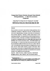
Fig. 1. The first experiment: foreground and background, (a): Original image (dyntex, ID = 647c610, frame 500), (b) & (g): GMM, (c) & (h): EGMM, (d) & (i): CRF, (e) & (j): SAGMM, (f) & (k): Our method.
And the variable sˆt,l is given by ρt,l sˆt,l = ρt,l
K � j=1
K � j=1
applied for background suppression. The various steps of our algorithm can be summarized as follows Step 1: Initialize the parameters Ψt = 2 2 , εt,l , υt,l } as follows: {πt,j , ρt,l , μt,j,l , σt,j,l 2 + The initialization of the parameters {πt,j , μt,j,l , σt,j,l } in our method are the same as that of GMM [1]. + The initial value of ρt,l is set to 0.95. �K 2 + Set εt,l = (K −1 j=1 μt,j,l )−1 and υt,l = � K 2 K −1 j=1 σt,j,l . Step 2: Evaluate the variables zˆt,j in (18) and sˆt,l in (20). Step 3: Update the parameters Ψt by using (23). It is worth mentioning that, for the learning rate β = (1 + t)−1 in (23), we have selected β = 0.01 for the for the first 400 frames. After that, we set β = (1 + t)−1 . Step 4: If there is a new observation, then go to step 2. To extract the foreground, we adopt the concept of background suppression in (6). The main difference is that we prune the feature set with ρt,l ≤ T p, and only select the feature with ρt,l > T p for background estimation. Where T p is a threshold. In the next section, we demonstrate the accuracy and effectiveness of the proposed model compared to others.
2 πt,j Φ(xt,l |μt,j,l , σt,j,l )
2 ) + (1 − ρ )Φ(x |ε , υ 2 ) πt,j Φ(xt,l |μt,j,l , σt,j,l t,l t,l t,l t,l
(20) 2 2 , εt,l , υt,l } B. Parameter Ψt = {πt,j , ρt,l , μt,j,l , σt,j,l
In order to update the parameter Ψt , we need to calculate the Fisher information matrix Ic (Ψt ) in (16). From (7) and (10), we have E[st,l ] = ρt,l and E[zt,j ] = πt,j
(21)
Now we can apply (21) to the Fisher information matrix Ic (Ψt ) in (16), after some manipulation, we have −1 −1 ; Ic (ρt,l ) = ρ−1 Ic (πt,j ) = πt,j t,l (1 − ρt,l ) 1 −2 −4 2 Ic (μt,j,l ) = πt,j ρt,l σt,j,l ; Ic (σt,j,l ) = πt,j ρt,l σt,j,l (22) 2 1 −2 −4 2 Ic (εt,l ) = (1 − ρt,l )υt,l ; Ic (υt,l ) = (1 − ρt,l )υt,l 2 Note that the prior probability πt,j should satisfy the con�K straints πt,j ≥ 0 and j=1 πt,j = 1. Apply (22) to (15), the 2 2 parameters Ψt = {πt,j , ρt,l , μt,j,l , σt,j,l , εt,l , υt,l } are updated as follows
πt,j = πt−1,j + (1 + t)−1 (ˆ zt,j − πt−1,j ) st,l − ρt−1,l ) ρt,l = ρt−1,l + (1 + t)−1 (ˆ μt,j,l = μt−1,j,l + (1 + t)−1 × −1 zˆt,j ρ−1 ˆt,l (xt,l − μt−1,j,l ) πt,j t,l s 2 2 σt,j,l = σt−1,j,l + (1 + t)−1 × −1 2 πt,j zˆt,j ρ−1 ˆt,l [(xt,l − μt−1,j,l )2 − σt−1,j,l ] t,l s −1 −1 εt,l = εt−1,l + (1 + t) (1 − ρt,l ) × (1 − sˆt,l )(xt,l − εt−1,l ) 2 2 υt,l = υt−1,l + (1 + t)−1 (1 − ρt,l )−1 × 2 (1 − sˆt,l )[(xt,l − εt−1,l )2 − υt−1,l ]
V. E XPERIMENTS In this section, the performance of the proposed method is compared to the GMM [1], EGMM [8], CRF [10], and SAGMM [11]. All compared methods are initialized similar to the initialization of the proposed algorithm. It is worth mentioning that the experiments do not consist of any pre/postprocessing step. Every algorithm was implemented and tested on a PC (i7, running at 2.79 GHz with 6 GB of RAM) in MATLAB environment. For our method, the thresholds (T h = 0.1 and T p = 0.95) are used in this paper. Except for CRF which uses 3 (K = 3) components, the number of components in all compared methods is assigned a value of 5 (K = 5). For all methods, the R, G, and B channels of the RGB color space are used in this paper (D = 3). In the first experiment, a real-world video from DynTex [21] is used to compare the performance of the proposed algorithm with others. This video contains 723 frames. In this
(23)
So far, the discussion has focused on estimating the parameter Ψt of the proposed model. Our online algorithm is
164
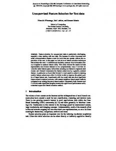
Fig. 2. The second experiment: foreground and background, (a): Original image (dyntex, ID = 647c510, frame 510), (b) & (g): GMM, (c) & (h): EGMM, (d) & (i): CRF, (e) & (j): SAGMM, (f) & (k): Our method.
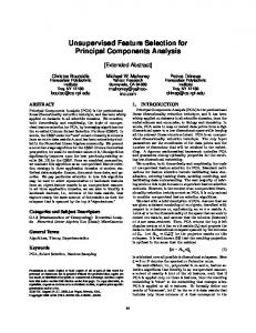
video, vehicles move at different speeds. Another difficulty in this experiment is that the sequence is very congested. Thus, the background road is difficult to be constructed due to the high amount of foreground present. From Figure 1(b) to (f), we present the background results at the frame 500 obtained by employing GMM, EGMM, CRF, SAGMM, and our method, respectively. It can be seen that the accuracy of the CRF method is poor compared to the GMM and EGMM. The SAGMM reduces the error significantly and can segment the background well. However, It can be seen that there is a “ghost” region that has been misclassified. The background road is well constructed by the proposed method in Figure 1(f). The foreground results are shown in Figure 1(g) to (k). In the next experiment, one real-world video clip with 641 frames, as shown in Figure 2(a), from the DynTex dataset is used. The original videos were downloaded from http://projects.cwi.nl/dyntex. From Figure 2(b) to Figure 2(f), we present the background results obtained by employing GMM, EGMM, CRF, SAGMM, and our method, respectively. In Figure 2(e), the SAGMM method demonstrates better performance compared to the GMM, EGMM, and CRF methods. Looking closely at the marked boxes of Figure 2(f), our method reduces the error significantly and can obtain the background well. As we mentioned in the previous sections, the advantage of our method is that it is allowing us to prune the feature set. In order to show this advantage, a video with 886 frames from Ztaki surveillance benchmark [22], as shown in Figure 3(a), is used. In this video, people stand, move across, and radially on the scene. In the first part of this experiment, we show the results of all compared methods when original video (without noise) is used. Figure 3(g) to Figure 3(k) present moving subtraction (absolute difference between original video and background) obtained by employing GMM, EGMM, CRF, SAGMM, and our method, respectively. Looking closely at the marked boxes, the result obtained by our method in Figure 3(k) is very similar with that of EGMM in Figure 3(h) and SAGMM in Figure 3(j). Now, in the second part of this experiment, instead of using the original video as in Figure 3(a), however,
the Gaussian noise (0 mean, 0.2 variance) are added to the R channel of the original video. In Figure 4(a) to Figure 4(c), we show the R, G, B channels at the frame 678. In this case, the G, B channels are useful, while the R channel should be irrelevant for modeling. In Figure 4(d)–(f), we show the moving subtraction obtained by employing EGMM, SAGMM, and our method, respectively. As we can see, the EGMM in Figure 4(d) and SAGMM Figure 4(e) are poor in this case. Our method with feature selection Figure 4(f) can automatically prune the R channel. A visual inspection of the result indicates that Figure 4(f) yields a better result compared to the two previous results. In order to look inside the feature saliencies ρt,l to see how it works. One video from Ztaki surveillance benchmark, as shown in Figure 5, is used in this experiment. This video has 1179 frames. In this experiment, from the frame 1 to frame 400, the Gaussian noise (0 mean, 0.2 variance) is added to the R channel. From the frame 401 to frame 1179, the Gaussian noise (0 mean, 0.25 variance) is added to the G channel. Clearly, In this case, from frame 1 to frame 400, the G, B channels are useful, while the R channel should be irrelevant for modeling. Also, from frame 401 to frame 1179, the R, B channels are useful, while the G channel should be irrelevant for modeling. In Figure 5(f), we show the average value of feature saliencies ρt,l for every pixel at each frame. As we can see, the same initial value is used for all feature saliencies at the first frame (t = 1). From frame 1 to frame 400, the feature saliency of the R channel is decreasing, whereas, the feature saliencies of the G, B channels are increasing. It is worth mentioning that the higher the value of feature saliency, the more important is the feature. In this paper, we prune the feature set with ρt,l ≤ T p, (T p = 0.95) and only select the feature with ρt,l > T p for background estimation. Based on this consideration, we can say that the R channel is not important from frame 1 to frame 400. Similarly, from Figure 5(f), we can see that, the G channel is not important from frame 423 to frame 1179. Figure 5(d) and Figure 5(e) present moving subtraction obtained by employing SAGMM and our method at the frame 390, respectively.
165
Fig. 3. The third experiment: background and moving subtraction, (a): Original image (Ztaki laboratory, frame 678), (b) & (g): GMM, (c) & (h): EGMM, (d) & (i): CRF, (e) & (j): SAGMM, (f) & (k): Our method.
Fig. 4. The fourth experiment: online unsupervised feature selection, (a): R channel (Gaussian noise, 0 mean, 0.2 variance), (b): G channel, (c): B channel, (d): EGMM, (e): SAGMM, (f): Our method.
In order to show the execution time comparison, one video is shown in Figure 6(a). This video contains 1203 frames. The image size of each frame is 144x176. All methods are evaluated on the same platform (MATLAB, i7, 2.79 GHz, 6 GB RAM), which is already mentioned earlier. As shown, SAGMM in Figure 6(j) is the quickest method taking 0.083s/frame. GMM in Figure 6(g) ranks second in the computation time with 0.093s/frame. Our method is quite slow with 0.136/frame. However, as shown Figure 6(k), the proposed method performs quite well for foreground and background compared to other methods.
model. The proposed method has been tested with real world videos. We demonstrate through extensive simulations that the proposed model is superior to other methods for background Suppression. One limitation of the work we have presented in this paper is the remaining parameter K. One possible extension of this work is to adopt the variational Bayesian learning to automatically optimize the parameter K. This is an open question and remains the subject of current research. ACKNOWLEDGEMENTS This research has been supported in part by the Canada Research Chair Program and the NSERC Discovery grant.
VI. C ONCLUSION We have presented an online unsupervised feature selection for moving object detection. The advantage of our method is that it is intuitively appealing. Also, it allows us to prune the feature set, avoids any combinatorial search, and does not require knowledge of any class labels. The online EM algorithm is adopted to estimate the unknown parameters of the proposed
R EFERENCES [1] Stauffer C. and Grimson W., “Adaptive background mixture models for real-time tracking,” in Proc. IEEE Conf. Comput. Vis. Pattern Recognit., 1999, pp. 246–252. [2] Vargas M., Milla J., Toral S., and Barrero F., “An enhanced background estimation algorithm for vehicle detection in urban traffic scenes,” IEEE Trans. Veh. Technol., vol. 59, no. 8, pp. 3694–3709, 2010.
166
Fig. 5. The fifth experiment: online unsupervised feature selection, (a): R channel (Aton, campus, frame 390), (b): G channel (Gaussian noise, 0 mean, 0.4 variance), (c): B channel, (d): SAGMM, (e): Our method, (f): The feature saliencies ρt,l .
Fig. 6. The sixth experiment: the computation time, (a): Original image (dyntex, ID = 645c510, frame 750), (b) & (g): GMM (time = 0.093s/frame), (c) & (h): EGMM (time = 0.101s/frame), (d) & (i): CRF (time = 0.374s/frame), (e) & (j): SAGMM (time = 0.083s/frame), (f) & (k): Our method (time = 0.136/frame).
[3] Kasturi R., Goldgof D., Soundararajan P., Manohar V., Garofolo J., Bowers R., Boonstra M., Korzhova V., and Zhang J., “Framework for performance evaluation of face, text, and vehicle detection and tracking in video: data, metrics, and protocol,” IEEE Trans. Pattern Anal. Mach. Intell., vol. 31, no. 2, pp. 319–336, 2009. [4] Lipton A. J., Fujiyoshi H., and Patil R. S., “Moving target classification and tracking from real-time video,” in Proc. IEEE Workshop App. Comput. Vis., 1998, pp. 8–14. [5] Huang J. C., Su T. S., Wang L.J., and Hsieh W. S., “Double-changedetection method for wavelet-based moving-object segmentation,” Electron. Lett., vol. 40, no. 13, pp. 798–799, 2004. [6] Han B., Comaniciu D., and Davis L., “Sequential kernel density approximation and its application to real-time visual tracking,” IEEE Trans. Pattern Anal. Mach. Intell., vol. 30, no. 7, pp. 1186–1197, 2008. [7] Greenspan H., Goldberger J., and Mayer A., “Probabilistic space-time video modeling via piecewise GMM,” IEEE Trans. Pattern Anal. Mach. Intell., vol. 26, no. 3, pp. 384–396, 2004.
[8] Lee D. S., “Effective Gaussian mixture learning for video background subtraction,” IEEE Trans. Pattern Anal. Mach. Intell., vol. 27, no. 5, pp. 827–832, 2005. [9] Zivkovic Z., “Improved adaptive Gaussian mixture model for background subtraction,” in Proc. IEEE Int. Conf. Pattern Recognit., 2004, pp. 28–31. [10] Wang Y., Loe K. F., and Wu J. K., “A dynamic conditional random field model for foreground and shadow segmentation,” IEEE Trans. Pattern Anal. Mach. Intell., vol. 28, no. 2, pp. 279 –289, 2006. [11] Chen Z. and Ellis T., “Self-adaptive Gaussian mixture model for urban traffic monitoring system,” in Proc. IEEE Int. Conf. Comput. Vis. Workshops, 2011, pp. 1769–1776.. [12] Law M. H., Figueiredo M. A. T., and Jain A. K., “Simultaneous feature selection and clustering using mixture models,” IEEE Trans. Pattern Anal. Mach. Intell., vol. 26, no. 9, pp. 1154–1166, 2004. [13] Vaithyanathan S. and Dom B., “Generalized model selection for unsupervised learning in high dimensions,” in Proc. Adv. Neural Inf. Process.
167
Syst., 1999, pp. 970–976. [14] Constantinopoulos C., Titsias M. K., and Likas A., “Bayesian feature and model selection for gaussian mixture models,” IEEE Trans. Pattern Anal. Mach. Intell., vol. 28, no. 6, pp. 1013–1018, 2006. [15] Li Y. H., Dong M., and Hua J., “Simultaneous localized feature selection and model detection for Gaussian mixtures,” IEEE Trans. Pattern Anal. Mach. Intell., vol. 31, no. 5, pp. 953–960, 2009. [16] McLachlan G. J. and Peel D., “Finite mixture models”, Wiley, 2000. [17] Bishop C. M., “Pattern recognition and machine learning”, Springer, 2006. [18] Titterington D. M., “Recursive parameter estimation using incomplete data,” J. R. Statist. Soc. B, vol. 46, no. 2, pp. 257–267, 1984. [19] Olivier C. and Eric M., “On-line expectation–maximization algorithm for latent data models,” J. R. Statist. Soc. B, vol. 71, no. 3, pp. 593– 613, 2009. [20] Allou S., Christophe A., and Gerard G., “An online classification EM algorithm based on the mixture model,” Stat. and Comput., vol. 17, no. 3, pp. 209–218, 2007. [21] Peteri R., Fazekas S., and Huiskes M. J., “DynTex: A comprehensive database of dynamic textures,” Pattern Recognit. Lett., vol. 31, no. 12, pp. 1627–1632, 2010. [22] Benedek C. and Sziranyi T., “Bayesian foreground and shadow detection in uncertain frame rate surveillance videos,” IEEE Trans. Image Process., vol. 17, no. 4, pp. 608–621, 2008.
168